CDS Rate Construction Methods by Machine Learning Techniques

CDS RATE CONSTRUCTION METHODS

by MACHINE LEARNING TECHNIQUES

Raymond Brummelhuis

Zhongmin Luo

[email protected]; [email protected]

Abstract

Regulators require financial institutions to estimate counterparty default risks from liquid CDS quotes for the valuation and risk management of OTC derivatives. However, the vast majority of counterparties do not have liquid CDS quotes and need proxy CDS rates. Existing methods cannot account for counterparty-specific default risks; we propose to construct proxy CDS rates by associating to illiquid counterparty liquid CDS Proxy based on Machine Learning Techniques. After testing 156 classifiers from 8 most popular classifier families, we found that some classifiers achieve highly satisfactory accuracy rates. Furthermore, we have rank-ordered the performances and investigated performance variations amongst and within the 8 classifier families. This paper is, to the best of our knowledge, the first systematic study of CDS Proxy construction by Machine Learning techniques, and the first systematic classifier comparison study based entirely on financial market data. Its findings both confirm and contrast existing classifier performance literature. Given the typically highly correlated nature of financial data, we investigated the impact of correlation on classifier performance. The techniques used in this paper should be of interest for financial institutions seeking a CDS Proxy method, and can serve for proxy construction for other financial variables. Some directions for future research are indicated. JEL Classification: C4; C45; C63

machine learning;CounterpartyCreditRisk;CDSProxy construction; classification

1

Introduction

1.1

A Shortage of Liquidity Problem

One important lesson learned from the 2008 financial crisis is that the valuation of Over-the-Counter (OTC) derivatives in financial institutions did not correctly take into account the risk of default associated with counterparties, the so-calledCounterparty Credit Risk(Brigoet al. 2103). To align the risk neutral valuation of OTC derivatives with the risks to which investors are exposed, the finance industry has come to recognize that it is critical to make adjustments to the default-free valuation of OTC derivatives using metrics such as Credit Value Adjustment (CVA), Funding Value Adjustment (FVA), Collateral Value Adjustment (ColVA) and Capital Value Adjustment (KVA) (altogether often referred to as XVA, see Gregory, 2015). In 2010, the Basel Committee on Banking Supervision (BCBS) published Basel III (BCBS, 2010) which requires banks to provide Value-at-Risk-based capital reserves against CVA losses, to account for fluctuations in the of market value of Counterparty Credit Risks. These have to be computed from market implied estimates of the individual counterparty’s default risks. Also, effective in 2013, the IFRS 13 Fair Value Measurement

∗

Universit´e de Reims-Champagne-Ardenne, Laboratoire de Math´ematiques EA 4535, Reims, France

†

Birkbeck, University of London and Standard Chartered Bank; the views expressed in the paper are the author’s own and do not necessarily reflect those of the author’s affiliated institutions.

issued by the International Accounting Standard Board (IASB, 2011) requires financial entities to report the market values for their derivative positions, including the market-implied assessment of Counterparty Credit Risks.

The calculation of both the CVA and of the associated regulatory capital requires the calibration of a counterparty’s term structure of risk-neutral default probabilities to liquid Credit Default Swap (or CDS) quotes associated with the counterparty. However, as highlighted in a European Banking Authority’s survey (EBA, 2015), among the Internal Model Method (or IMM) compliant banks, over 75% of the counterparties do not have liquid CDS quotes. We refer to the problem of assessing the default-risk of counterparties without liquid CDS quotes as theShortage of Liquidity problem, and to any method to construct the missing quotes on the basis of available market data as aCDS Rate Construction Method.

One recommended solution-method for this Shortage of Liquidity problem is to map a counter-party lacking liquidly quoted CDS spreads to one for which a liquid market for such quotes exists, and which, according to criteria based on financial market data, best resembles the non-quoted party. The CDS data of the liquid counterparty, which is called aproxyof the non-liquid counter-party, can subsequently be used to obtain estimates for the risk-neutral default probabilities of the latter. Following practitioners’ usage, we will refer to this as aCDS Proxy Method. We will refer to the counterparties having liquid CDS quotes asObservablesand those without liquid quotes asNonobservables. We note in passing that often, in practice, if, for a given day, the number of a counterparty’s CDS quotes from available data vendors such as MarkITTM_{(or others) falls below a}

certain threshold, the counterparty is deemed to be illiquid.

As we will see below, current methods for constructing CDS proxy rates follow a different route, in that they seek to directly construct the missing rates, based on Region, Sector and Ratings data. They treat all counterparties in a given Region, Sector and Ratings bucket homogeneously and therefore typically fail to pick up counterpart-specific default risk, thereby failing some of the European Banking Authority’s criteria for a sound CDS proxy-rate construction method. In this paper we will, amongst other things, enlarge the set of financial market data used for CDS Proxy construction to include both stock and options market data. We also replace ratings by estimated default probabilities. It might have been considered natural to also include corporate bond spreads in this list, but we decided not to do so because of the relative lack of liquidity in the corporate bond market: Longstaffet al. (2005) concluded from a comprehensive empirical study of CDS spreads and the corresponding bond spreads that there exists a significant non-default component in corporate bond spreads due to illiquidity, as measured by the bid-ask spreads of corporate bonds. As highlighted by Gregory (2015), the vast majority of the counterparties of banks do not have liquid bond issues and the liquidity of bonds is generally considered to be poorer than that of the CDS contracts associated with the same counterparties. Therefore, a bond-spread based CDS Proxy Method will not be particularly helpful for solving the Shortage of Liquidity problem. That being said, it would be easy to include such bond spread variables into any of the CDS Proxy methods we introduce and examine in this paper.

Another contribution of this paper is that we go beyond the traditional regression approach commonly used in Finance, and construct our CDS Proxies using classification algorithms which were developed by the Machine Learning community, algorithms whose efficiency we tested and whose relative performances we rated. As discussed below, there is little published research on the Shortage of Liquidity problem and its solution. One of the motivations of this paper is to address what seems to be an important gap in the literature, by providing and examining alternatives to the few currently existing CDS Rate Construction Methods.

1.2

Regulators’ Criteria for Sound CDS Proxy Methods

1. The CDS Proxy Method has to be based on an algorithm that discriminates at least three types of variables: Credit Quality (e.g., rating), Industry Sector and Region (BCBS, 2015).

2. Both the Observable Counterparties used to construct a CDS proxy spread for a given Nonob-servable and the NonobNonob-servable itself have to come from the same Region, Sector and Credit Quality group (BCBS, 2015).

3. According to (EBA, 2013), the proxy spread must reflect available credit default swap spreads. In addition,the appropriateness of a proxy spread should be determined by its volatility and not by its level. This criterion highlights the regulators’ requirement that CDS proxy rates should include counterparty-specific components of counterparty default risk, which are not adequately measured by purely level-based measures such as an average or median of a group of CDS spreads or region- or industry-based CDS indices.

We next take a look at existing CDS Proxy Methods. A survey of the publicly available literature showed that the following two types of CDS Proxy Methods are currently used by the finance industry:

• _{TheCredit Curve Mapping Approach described in Gregory (2015), which simply creates} Re-gion/Sector/Rating buckets consisting of single-name CDS contracts with underlying refer-ence entities from the same regions and sectors and with the same ratings, and then proxies the CDS rates of a Nonobservable from a given Region/Sector/Rating bucket by the mean or median of the spreads of the single-name CDS rates within that bucket. This approach clearly satisfies criteria #1 and #2 but assumes the counterparty default risks for all counterparties coming from the same Region, Sector and Rating bucket to be homogeneous and ignores the idiosyncratic default risk specific to individual counterparties. In particular, using bucket average or median as Proxy CDS rate for a Nonobservable ignores the CDS-spread volatility across counterparties within the bucket, thereby failing to meet criteria #3.

• _{TheCross-sectional Regression Approachof Chourdakiset al. (2013): this is another popular} CDS Proxy Method which assumes that an observable counterpartyi’s CDS rateSi (for a

CDS contract with given maturity and payment dates) can be explained by the following log-linear regression equation:

log(Si)=β0+ #Regions

X

m=1

βR mIiR,m+

#Sectors

X

m=1

βS mIiS,m+

#ratings

X

m=1

βr mIri,m+

#seniorities

X

m=1

βs

mIsi,m+i, (1)

where theI’s s are dummy or indicator variables for, respectively, sector, region, rating class and seniority, as specified in the CDS contract. The regression-coefficients can be estimated by Ordinary Least Squares, withi representing the estimation error. Once estimated, the

regression can be used to predict the rate of a CDS-contract of a Nonobservable in a given region and sector with a given rating and seniority. The Cross-sectional Regression Approach goes beyond the Curve Mapping Approach in that it provides a linkage between CDS Rates and the above five explanatory variables, which goes beyond simply taking bucket means. However, like the Curve Mapping Approach, its predictions still treat the market-implied default risks for counterparties within the same Region, Sector, Rating and Seniority bucket homogeneously and as such ignores counterparty-specific risks. The Cross-sectional Regres-sion Approach proxies the counterparty’s CDS spread by an expected value coming from a regression; it provides the level of a CDS spread but ignores the CDS-spread volatility among individual counterparties and therefore does not satisfy criteria #3 either.

critical ingredient of any statistical modelling approach. The different Machine Learning-based CDS Proxy Methods we introduce and investigate in this paper do take idiosyncratic counterparty default risk into account. Moreover, we performed extensive out-of-sample tests for each of the methods we investigated using Stratified Cross Validation. We briefly describe what we believe are the main contributions of this paper to the existing literature.

1.3

Contributions of the Present Paper

To tackle the Shortage of Liquidity problem, we apply Machine Learning Techniques, and more specifically, Classification Techniques, using the best known Classifier families in the Machine Learning area: Discriminant Analysis (Linear and Quadratic), Na¨ıve Bayesian,k-Nearest Neigh-bourhood, Logistic Regression, Support Vector Machines, Neural Networks, Decision Trees and Bagged Trees. We call this approach the Machine Learning based CDS Proxy Method. To the best of our knowledge, this paper represents the first research in the public domain on applications of Machine Learning techniques to the Shortage of Liquidity Problem for CDS rates.

Furthermore, given the wide range of available Classifiers and their parametrisations choices, the question of comparing the performances of different classifiers naturally arises. We have carried out a detailed classifier performance comparison study across the different Classifier families (referred to as Cross-classifier Comparison below) and also within each Classifier family (referred to as Intra-classifier Comparison). As far as we are aware, this is the first empirical comparison of Machine Learning Classifiers based entirely on financial market data. To clarify this point, we briefly review some of the existing Classifier Comparison literature. Readers who are unfamiliar with the Machine Learning-terminology used in this section may refer to Section 2 for clarification. STATLOG by Kingat al. (1995) is probably the best known empirical classifier comparison study for a comprehensive list of classifiers. One conclusion drawn from that study is that clas-sifier performance can vary greatly depending on the type of dataset used, such as sector-type: Medical Sciences, Pharmaceutical Industries and others, and that researchers should rank classi-fiers’ performance for the specific type of data set which is the subject of their study. As mentioned, we believe ours to be the first such study for financial market data.

Delgado and Amorim (2014) is a more recent contribution to the classifier comparison literature. It compared 179 classifiers from 17 families based on 121 datasets, usingMaximum Accuracyas the criterion to identify the top performing classifier families. As emerged from their study, these were, in descending order of performance, the Random Forest (an example of a so-called Ensemble Classifier), the Support Vector Machine, more specifically with Gaussian or Polynomial Kernels, and the Neural Network. All of these will be presented in some detail in Section 2 below, except for the Random Forest algorithm, which in our study we replaced with another Ensemble Classifier, the Bagged Tree.

Classifier families) or negative, for Na¨ıve Bayes and for some of the LDA and QDA classifiers. We have compared a total of 156 classifiers from the eight main families of classifier algorithms mentioned above, with different choices of parameters (which can be functional as well as numer-ical) and different choices of feature variables, for the construction of CDS Proxies on the basis of financial data from the 100 days up to Lehman’ bankruptcy. Our Cross-classifier comparison shows that for the construction of these Proxies, the three top-performing classifiers are the Neural Network, the Support Vector Machine and the Bagged Tree. A graphical summary of our results is given in Figure 10. This performance result is broadly consistent with that of both Kingat al. (1995) and Delgado and Amorim (2014). As part of ourIntra-classifierperformance comparison, we have compared classifiers within a single family with different parameterisations and different feature variables and found that this performance typically varies greatly, though for certain Classifier families, such as the Neural Networks, it can also be relatively stable. The empirical results are further discussed in Section 3, on the basis of graphs and tables which are collected in Appendix B. Although the different Classifier algorithms produced by the Machine Learning community can be used as so many ‘black boxes’ (which is arguably one of their advantages, from a user’s perspective), we believe that is also important to have at least a basic understanding of these algorithms, for their correct use and interpretation, and also to understand their limitations. For this reason we have included a section where we present each of the eight Classifier families we have used, in the specific context of the problem we are addressing here.

1.4

Structure of the Paper

The rest of the paper is organized into three Sections plus two Appendices:

• _{In Section 2, we give a brief introduction to Machine Learning classification with a description} of each of the eight families of classifier algorithms we have used, alongside an illustrative example in the framework of our CDS Proxy Construction problem.

• _{In Section 3, we present the results of our cross-classifier and intra-classifier performance} comparison study for the construction of CDS Proxies.

• _{Section 4 presents our conclusions and provides some directions for future research.}

• _{Appendix A, finally, gives a detailed description of the six feature selections which are at the} basis of our Proxy constructions, and describes the data which we have used, while Appendix B contains the different graphs and tables related to individual classifier performances needed for the discussion of section 3.

2

Classification Models

Compared with traditional statistical Regression methods,Machine LearningandClassification Tech-niquesare not as well-known in the Finance industry and, for the moment at least, less used. This section introduces the basic concepts of Machine Learning and presents the eight classification algorithms which we used for our CDS Proxy construction. As a general reference, Hastieet al.

(2009) provides an excellent introduction to Classification and to Machine Learning in general. Although our paper focuses on the CDS Proxy Problem, its general approach can easily be adapted for the construction of proxies for other financial variables for which no or not enough market data are available.

The general aim of Machine Learning is to devise computerised algorithms which predict the value of one or moreresponse variableson a population each of whose members is characterised by a vector-valuedfeature variablewith values in some finite dimensional vector spaceRd.For our CDS

variables such as region, sector or rating class, and continuous variables such as historical and implied equity volatilities and (objective) Probabilities of Default or PDs, all over different time-horizons. We will sometimes add the 5-year CDS rate to this list, which is the most quoted rates, and therefore may be available for counterparties for which liquid quotes for the other maturities are missing.

The construction of the feature space should be based on its statistical relevance and on the economic meaning of the feature variables. For the former, formal statistical analysis can be conducted to rank-order the explanatory power of each of the feature variables regarding the response variable. As regards their economic relevance, one can apply business judgement, and also use available research on explanatory variables for CDS rates. A further important issue for us was that the features used should be liquidly quoted for the nonobservable counter parties as well as the observable ones. In our study, we have selected six sets of feature variables on the basis of which we constructed our CDS proxies, and we refer to Appendix A for their description and for some further comments on how and why we selected them as we did. Our selection is not meant to be prescriptive, and in practice a user might prefer other features.

The relevant response variable could be a CDS rate of a given maturity, as in the two existing CDS Proxy Methods mentioned in section 1.2, or it could be a class label, such as the name of an observable counterparty. This already shows that the response variable can either becontinuous, in which case we speak of aRegression Problem, or discrete, in which case we are dealing with a

Classification Problem. In this paper we will be uniquely concerned with the latter.

Unlike Regression-based approaches, the Classification-based CDS Proxy Methods we investi-gate in this paper do not attempt to predict the CDS rates of the different maturities. Instead, they associate an observable counterparty to a non-observable one based on a set of (financial) features which can be observed for both. The, liquidly quoted, CDS rates of the former can then be used for managing the default risk of the latter, such as the computation of CVAs and of CVA reserve capital. As compared to regression, a Classification-based CDS Proxy method has the advantage of ultimately only using market-quoted CDS rates, which therefore, in principle at least, are free of arbitrage. By contrast, using a straightforward regression for each of the different maturities for which quotes are needed risks introducing spurious arbitrage opportunities across the different maturities: see Brummelhuis and Luo (2017). It in fact turns out to be remarkably difficult to precisely characterise arbitrage-free CDS term structures even for a basic reduced-form credit risk model (though simple criterions for circumventing ”evident” arbitrages can be given). On the other hand, such a characterisation would seem to be a necessary pre-requisite for an guaranteed arbitrage-free regression approach. We make a number of further observations.

1. Depending on the type of classifier, the strength of the association between an observable and a nonobservable counterparty can be defined and analysed statistically. For example, Linear Discriminant Analysis which, going back to R. A. Fisher in 1936, is one of the oldest classifier algorithms known, estimates the posterior probability for a nonobservable to be classified into any of the observables under consideration, given the observed values of the feature variables. It then chooses as CDS Proxy that observable for which this posterior probability is maximal: see subsection2.1 below for details.

2. The different classifiers will be calibrated on Training Sets, and their performances evaluated by a statistical procedure know asK-fold Stratified Cross Validation: see section 2.10 below for a description. Depending on the strength of the statistical association and the results of the cross-validation, one can then argue that the nonobservable will, in its default risk profile, resemble the observable to which has been classified.

only. The different PDs might be provided by a Credit Rating Agency or be a bank’s own internal ratings.

4. We ultimately take as missing CDS rates for a Nonobservable counterparty the, market-quoted, CDS rates of the Observable to which it is most strongly associated by the chosen Machine Learning algorithm, on the basis of the values of its feature variables (where the precise meaning of ”association” will depend on the algorithm which is used). In view of the previous point, these proxy rates will automatically reflect Region and Sector risk, and thereby satisfy the regulators’ criteria #1 and #2 mentioned in subsection 1.2 above. Our approach also addresses the regulators’ criterion #3: the proxy rates will be naturally volatile, as market-quoted, rates of the selected Observable. Furthermore, they will also reflect the Nonobservable’s own counterparty-specific default risk since, as market conditions evolve, the non-observable may be classified to different observables depending on the evolution of its feature variables.

To give a more formal description of a Classification algorithm, let {₁, . . . ,_N} _{be the set of} Observables, which we therefore label by natural numbers, and letRdbe the chosen feature space.

A typical feature vector will be denoted by a boldface x = (x1, . . . ,xd). As mentioned, for us

the components of the feature vector will be financial variables such as as historical or implied volatilities and/or estimated PDs, over different time horizons. Our Classification problem is to construct a mapby:R

d_{→ {1, . . . ,N}based on a certaintraining setof data,}

DT ={_(xi,_{yi) :xi}∈_Rd,_yi∈ {₁, . . . ,_N}, _i=₁, . . . ,_n}, ₍₂₎

corresponding to data on Observable counterparties: xi is an observed feature vector of

coun-terparty yi.Each of the Machine Learning algorithms we will use is, mathematically speaking, a

recipe for the construction of a mapFθ :Rd → {1, . . . ,N}, withθa vector of parameters, and our

mapsbywill be of the form:

by(x)=Fbθ(x) (3)

where the parametersθbwill be ”learned” from the training setDT, usually by maximising some

performance criterion or minimising some error, depending on the type of Learning algorithm used. The parametersθcan be numerical, such as thekin thek-Nearest Neighbour method, the tree size constraint in the Decision Tree algorithm or the number of learning cycles for the bagged Tree, but also functional, such as the kernel function in the Na¨ıve Bayesian method, the kernel function of a Support Vector Machine, or the activation function of a Neural Network. Where possible, we have optimised numerical parameters by cross-validation.

We note in passing that the constructed classifier mapby will in general of course strongly

depend on the training set and a more complete , though also more cumbersome, notation such as

byDT (orbθDfor the optimal parameters) would have indicated this dependence; we will however

leave it as implicitly understood. In practice there would also be the question of how often we would need to update these training sets: this would amongst other things depend on the speed with which the classification algorithm ”learns” - determines the

Following Machine Learning literature such as Delgado and Amorim (2014), we refer to the classification algorithms that are based on the same methodology as aClassifier Family. Within each Classifier Family, we refer to classification algorithms that differ from each other by their parameterisations, including the dimensionality of the feature vectors, as the individualClassifiers. As shown in later sections, exploring parameterisation choices not only serves to choose the best classifier based on classification performance, it is also helpful to explain performance variations across classifiers.

headings ”FS1-FS6” in the third column refers to the 6 different feature variable selections we have used and which are detailed in Appendix A.

In the remainder of this section, we introduce the eight most popular Classifier Families of Machine Learning (Wuet al., 2008) , in the specific context of the CDS Proxy problem, together with some illustrative examples. At the end of the section we present the statistical procedure we used for cross validation and Classifier selection. We next turn to a description of each, with illustrative examples.

2.1

Linear Gaussian Discriminant Analysis

Linear Discriminant Analysis or LDA, as well as the closely related Quadratic Discriminant Anal-ysis (QDA) and Na¨ıve Bayesian Method (NB) which we will discuss below, are based on Bayes’ rule. These methods interpret the training setDT _={(x

i,yi) :i=1, . . . ,n}as a sample of a pair of

random variables (X,Y), and estimate the posterior probability density that a feature vectorx is classified into the class (for us, counterparty)jby Bayes’ formula,

P(Y= j|X =x)= P(X =x

|_Y=_j)P(Y= _j)

P(X) ,

whereP(X=x|Y= j) is a prior probability density on the feature vectors belonging to the class j,

which we will also call theclass-conditional density, and whereP(X)=PNk=1P(X |Y=k)P(Y=k).

To simplify notations we will often writeπj := P(Y = j) for the, unconditional, probability of

membership of classj,P(x|_{j) forP(X} =_x|_Y= _{j) andP(j}|_{x) forP(Y}= _j|_X=_x).

The LDA, QDA and NB methods differ in their assumptions on the class-conditional densities. For the first two these densities are assumed to be Gaussian. One can generalize the LDA and QDA methodologies to include non-Gaussian densities, e.g. by using elliptical distributions, but the resulting decision boundaries (defined below) would no longer have the characteristic of being the linear or quadratic hyper surfaces which give their name to LDA and QDA. We refer to Hastie

et al.(2009) for a general introduction to Bayesian Classifications based on Bayes’ formula.

2.1.1 The LDA algorithm

Linear Discriminant Analysis defines the classjconditional density function to be

fj(x) :=P(X=x|Y= j) :=(2π)−

d

2|V|− 1 2e−

1 2(x−µj)TV

−1_(x−µ

j), ₍₄₎

whereµj represents the mean of the feature vectors associated to the j-th class and whereV is

a variance-covariance matrix with non-zero determinant|_V| _{and inverse V}−1_{.Observe that we}

are takingclass-specificmeans but anon-class-specificvariance-covariance matrix. Taking the latter class-specific also leads to QDA, which will be discussed in subsection 2.2 below.

As a natural choice forµjandVwe can, for a given training data setDT ={xi,yi) :i=1, . . . ,n},

take forµjthe sample mean of the feature vectors associated to classj,

µj= 1

nj

X

i:yi=j xi,

wherenj := #{(xi,yi) : yi = j} is the number of data points in class j, and for V be the sample

We finally need the prior probabilitiesπjfor membership of classj; again, several choices are

possible. We have simply taken the empirical probability implied by the training set by putting

πj=nj/n, where we recall thatn=#DTis the number of data points, but, alternatively, one could

impose a Bayesian-style uniform probabilityπj=1/N(which would be natural as an initial a-priori

probability if one would use Bayesian estimation to train the algorithm). Finally, one can estimate theπj’s by Maximum Likelihood, simultaneously with the other parameters above.

Once calibrated or ”learned”, a new feature vectorxis classified as follows: the log-likelihood ratio thatxbelongs to classjas opposed to classlcan be expressed as:

L_{j,l(x) :}=_log fj(x)πj/P(x)

fl(x)πl/P(x)

!

=log (πj/πl)+logfj(x)−logfl(x)

=log(πj/πl)−

1 2µ

T jV

−1_µ

j+

1 2µ

T

lV

−1_µ

l+xTV

−1_(µ

j−µl). (5)

This is an affine function ofxand the decision boundary, which is obtained by settingL_{j,l(x) equal} to 0, is therefore a hyperplane inRd.If we define the discriminant function for classjby

dj(x)=xTV−1µj− 1 2µ

T

jV −1_µ

j+logπj, (6)

thenL_j,l(x)> _{0 i}ff_dj(x) >_{dl(x), in which case the feature vectorxis classified to observable jas} opposed to l.This is the LDA criticism for classification into two classes. To generalise this to multi-class classification, we classify a feature vectorxinto the classjto which it has the strongest association as measured by the discriminant functions (6): our optimal decision rule therefore becomes

by(x)=arg max

j dj(x). (7)

This is also known as theMaximum A Posteriorior MAP decision rule; the same, or a similar, type of decision rule will be used by other classifier families below.

2.1.2 An Illustrative Example

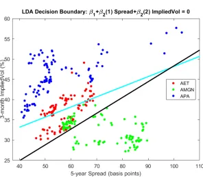
To illustrate the two DA algorithms and NB we use the example of three counterparties called AET, APA and AMGN, for which we have observed two-dimensional feature vectorsx=(s, σimp_3m) repre-senting the 5-year CDS rate and the 3-month implied volatility. In Figure 1 the observed feature vectors of APA are plotted in blue, and those of AET and AMGN in red and green, respectively. The cyan line is the resulting LDA decision boundary discriminating between APA and AMGN while the dark line discriminates between AET and AMGN. We have omitted the third decision bound-ary for better lisibility of the graph. Clearly, the LDA does a better job discriminating between APA and AMGN than between AET and AMGN. To classify a nonobservable counterparty, one first computes the ”scoring functions” (6), withj=1,2,3 corresponding to the three observables, APA, AMGN and AET, respectively, and associates the counterparty to thatjfor which the score is maximal (and for example to the smallestjfor which the score is maximal in the exceptional cases there are several such j).

As indicated in Table 1, we have investigated two types of LDA classifiers with two different parameterisation choices for the pooled variance-covariance matrixV, one imposing a diagonal

Figure 1: Linear Discriminant Analysis

2.2

Quadratic Discriminant Analysis

LDA assumes that the variance-covariance matrix of the class-conditional probability distributions is independent of the class. By contrast, in Quadratic Discriminant Analysis (QDA) we allow a class-specific covariance matrixVj for each of the classes j. As a result, we will get quadratic

decision boundaries instead of linear ones.

2.2.1 The QDA algorithm

Under the Gaussian assumption, the class conditional density functions for QDA are take to be:

fj(x)=P(X=x|Y= j)=(2π)−

d

2|V

j|

−1 2e−

1

2(x−µj)TV_j−1(x−µj)_,

(8)

where nowVjis a class-specific variance-covariance matrix andµj, as before, a class-specific mean.

As for LDA, there are several options for calibrating the model; we simply took the sample mean and variance-covariance matrix of the set{_xi:yi= _j}.

Comparing log-likelihoods of class memberships as we did for LDA now leads to quadratic discriminant functionsdjgiven by

dj(x)=−1

2log|Vj| − 1 2(x−µj)

T_V−1

j (x−µj)+logπj. (9)

A feature vectorxwill be classified to classjrather thanlifdj(x)>dj(xl), and the decision boundaries

{_{x : dj(x)} = _dl(xl)}_{will now be quadratic. The Decision Rule for multi-class classification under} QDA is again the MAP rule (7), but with the new scoring function (9). IfVj = Vl for allland j,

2.2.2 An Illustrative Example for Quadratic Discriminant Analysis

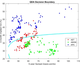
The cyan curve in Figure 2 depicts the quadratic decision boundary between counterparties APA and AMGN of example 2.1.2 as found by the QDA algorithm, where for the purpose of better presentation we only show one of the three decision boundaries.

Figure 2: An Example for Quadratic Discriminant Analysis

As indicated in Table 1, we have investigated two QDA classifiers with, as for LDA, two parametrisation choices for the covariance matrices Vj, diagonal and full, for the six different

Feature Variable Selections. Cross-classifier and intra-classifier comparison results can be found in Section 3 and Appendix B. In particular, Figure 12 shows that for our CDS Proxy problem, QDA with full variance-covariance matrices outperforms the other DA algorithms across all six Feature Selections, where the difference in performance can be up to around 20% in terms of accuracy rates.

2.3

Na¨ıve Bayes Classifiers

As for LDA and QDA, Na¨ıve Bayes Classifiers calculate the posterior probabilitiesP(j| x) using

Bayes’ formula, but make the strong additional assumption that, within each class, the components of the feature variables act as independent random variables: given thatY = j, the components

X_ν of X are independent, ν = 1, . . . ,d. In other words, the individual features are assumed to be conditionally independent, given the class to which they belong. As a consequence of this

Class Conditional Independence assumption, Na¨ıve Bayes reduces the estimation of the multivariate probability densityP(x| j) to that of thedunivariate probability densities,

fj,ν(x) :=P(Xν=x|Y=j), ν=1, . . . ,d,

2.3.1 The NB decision algorithm

Under the Class Conditional Independence assumption, the classjconditional density is

fj(x)= d

Y

ν=1

fj,ν(xν). (10)

The log-likelihood ratio (5) can be evaluated as

L_j,l(x)=_log πjfj(x)

πlfl(x)

!

=logπj

πl + d

X

ν=1

logfj,ν(xν)−logfl,ν(xν

, (11)

with the decision boundaries again being obtained by settingL_{i j(}x) equal to 0. The discriminant functions of Na¨ıve Bayes are therefore

dj(x)=logπj+ d

X

ν=1

logfj,ν(xν), (12)

and the classifier of Na¨ıve Bayes, once calibrated or trained, is again defined by the MAP-rule (7).

There remains the question of how to choose the univariate densities fj,ν(xν).There are two

basic methods:

1. Parametric specification: one can simply specify a parametric family of univariate distributions for each of the fj,νand estimate the parameters from a training sample. Note that NB with normal fj,ν reduces to the special case of QDA with diagonal variance-covariance matrices

Vj.

2. Non-parametric specification: alternatively, one can employ a non-parametric estimator for the

fj,νsuch as the Kernel Density Estimator (KDE). We recall that if{x1,x2, . . . ,xn}is a sample

of a real-valued random variableXwith probability density f, thenParzen’s Kernel Density Estimatorof f is defined by

b f(x)= 1

nb

n

X

i=1

K _x−x

i

b

, (13)

where thekernel Kis a non-negative function onRwhose integral is 1 and whose mean is 0,

andb>0 is called thebandwidth parameter.

Kernel Density Estimators represent a way to smooth out sample data. The choice ofbis critical: too small abwill lead to possibly wildly varying fbwhich try to follow the data too closely, while

too large abwill ”oversmooth” and ignore the underlying structure present in the sample. Three popular kernels are the Normal kernel, whereK(x) is simply taken to be the standard normal pdf, and the so-called Triangular kernel and the Epanechnikov kernel (Epanechnikov, 1969), which are compactly supported piece-wise polynomials of degree 1 respectively 2, and for whose precise definition we refer to the literature. For simplicity we have used the same kernel and bandwidths for all fj,ν.

Our Intra-classifier comparison results show that the KDE estimator with Normal kernel out-performs other the two kernel functions in most cases. Regarding the choice of kernels and of bandwidths, for us the issue is not so much whether the KDE estimator provides good approxi-mations of the individual fj,ν’s but rather how this affects the classification error: in this respect,

2.3.2 An Illustrative Example for Na¨ıve Bayes

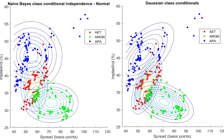
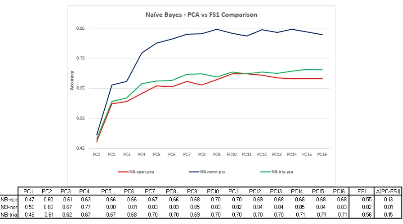
Figure 3 compares the contour plots of the class conditional densities found by NB with normally distributed individual features (graph on the left) with the ones found by QDA (graph on the right) for our example 2.1.2. The three normal distributions on the left have principal axes parallel to the coordinate axes, reflecting the independence assumption of Na´ıve Bayes. They show a stronger overlap than the ones on the right, whose tilted orientation reflects their non-diagonal covariance matrices. The stronger overlap translates into higher misclassification rates, and our empirical study confirms that Na¨ıve Bayes Classifiers perform less well than QDA for any of the feature variable selections used.

Figure 3: Naive Bayes Class Conditional Independence vs Correlated Gaussian

As listed in Table 1, we investigated the effects of Bandwith and Kernel function choices on Na¨ıve Bayes’ classification performance. Our empirical results in Section 3 show that Na¨ıve Bayes Classifiers perform rather poorly in comparison with the other Classifier families, in contrast with results from the literature on classification with non-financial data: see for example Rishet al.(2001) . This is probably due to the independence assumption of Na¨ıve Bayes, which is not appropriate for financial data: as indicated in Figure 15, for our data set, which came from a period of financial stress, roughly 80% of the pairwise correlations of our feature variables are above 70%. Even under normal circumstances one expects a 3-month historical volatility and a 3-month implied volatility to have significant dependence. The interested readers can find more details on the performance of NB in Appendix B.

2.4

k

-Nearest Neighbours

k-Nearest Neighboursork-NN algorithm is an example of a so-calledlazy learning strategy, because it makes literally zero efforts during the Training stage; as a result, it tends to be computationally expensive in the Testing/Prediction stage.

2.4.1 Thek-NN algorithm

LettingDT _{= {(x}

i,yi) :i =1, . . . ,n}be, as before, our Training Set, where for usxi is an observed

feature vector of the observable counterpartyyi, thek-NN algorithm can be described as follows:

• _{For a given feature vector x, which we can think of as the feature vector of some} non-observable name, compute all the distancesd(x,xi) for (xi,yi)∈ DT, where the metricd can

be any metric of one’s choice on the feature spaceRd, such as the Euclidean metric or the

so-called City Block metric.

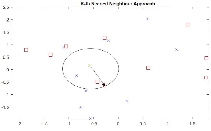
• _{Rank order the distances and select theknearest neighbours ofxamongst thexi}._{Call this set} of points<_(x,_{k): in Figure 4 these are the points within the circle.}

• _{Classifyx to that element}

by(x) ∈ {1,2, . . . ,N}which occurs most often amongst the yi for

whichxi ∈ <(x,k), with some arbitrary rule if there is more than on such an element (e.g.

taking the smallest). This is called theMajority Vote Rule; see Hastieet al.(2009) for a Bayesian justification.

As already mentioned, and in contrast in contrast to the other algorithms we considered, the

k-NN algorithm requires no training, and can immediately start to classify any feature vector whether in the training set or not.

2.4.2 An Illustrative Example fork-NN

Figure 4 provides a simple illustration of thek-th Nearest Neighbour algorithm. Based on a 2-dimensional feature space, it depicts the feature vectors of two observables, each with 10 data samples inside a rectangular box: one observable is represented by blue ”x” shapes; the other by red ”” shapes. Suppose we want to usek-NN to classify the nonobservablexrepresented by the grey cross. Takingk=3 and the Euclidean distance as metric, we find that the third nearest point toxwithin the Training set happens to be the red ”” to which the arrow points. Amongst these three nearest neighbours, the red boxes occur twice and the blue boxes only occur once. By the Majority Vote Rule, the CDS-Proxy forxis then selected to be the (name represented by) the red boxes.

As indicated in Table 1, we investigated k-NN with three different distance metrics, the Eu-clidean metric, the City Block or`1-metric and the so-called Mahalanobis distance which takes into account the spatial distribution (spread and orientation) of the feature vectors in the training sample1_{, and we studied the dependence of the classification accuracy onk.The Intra-classifier}

results are presented in figure 16 and in table 8 of Appendix B, and the comparison ofk-NN with the other Classifier families is done in Section 3.

2.5

Logistic Regression

In the Bayesian-type classifiers discussed so far, we have estimated the posterior probability den-sitiesP(j | x) by first modelling and estimating the feature vectors’ class-conditional probability

distributions, together with the prior probabilities for class membership, and then applying Bayes Formula. By contrast, Logistic Regression (LR) straightforwardly assume a specific functional

1_{The explicit formulas are: d} 2(x,y)=

p

(x−_y)T_(x−_y= pP_ν(xν−_yν)2_{for the Euclidean metric,d1(x,y)=}P

ν|xν−_yν|

for the City Block metric, anddV =

q

(x−_y)T_bV−₁

(x−_{y) for the Mahalanobis metric, where}bVis the empirical

Figure 4:k–NN Illustrative Example

form forP(j|x) which then is directly estimated from the training data. Logistic Regression

clas-sifiers come in two types, Binomial and Multinomial, corresponding to two-class and multi-class classification.

2.5.1 Binomial LR Classification

Suppose that we have to classify a feature vectorx∈_Rd_{to one of two classes,Y=0 or 1.Binomial}

Logistic Regression assumes that the probability thatY=1 givenxis given by

p(x;β) :=P(Y=1|x) :=g

     β0+

X

ν

βνxν

     =g

βTx˜, (14)

where g(z) = (1+e−z₎−1

is the Logistic or Sigmoid function, β = (β0, β1, β2, . . . , βd) is a vector of

parameters and ˜x:=(1,x), the component 1 being added to include the intercept termβ0.Given a

training setDT = {_(xi,_yi)| _i=₁, . . . ,_n}_{with yi} ∈ {₀,₁}_{, the likelihood of obtaining the data ofD}T under this model can readily be written down, andβcan be determined by Maximum likelihood Estimation (MLE), for which standard statistical packages are available.

Once calibrated to parametersβbwe classify a new feature vectorxtoY=1 ifp(x,βb)≥0.5, and

toY=0 otherwise.: equivalently, since both probabilities sum to 1,

by(x)=arg max

j pj(x,βb),

wherep1(x,βb) := p(x,βb) and p₀(x,βb) = 1−p(x,βb) and where we agree to classifyx to 1 if both

probabilities are equal.

2.5.2 Multinomial LR Classification

To extend the two-class LR algorithm to the multi-class case, we recast a multi-class classification problem as a sequence of two-class problems. For example, we can single out one of the observables

between membership or no-membership of the reference class, that is, we takeY=1 ifxbelongs to this classj, andY=0 otherwise. This will result inN−_{1 logistic regressions withN}−_{1 parameter} vectorsβb_j,j=1, . . . ,N−1.The likelihoods that a new feature variablexwill be classified tojthen

isp(x,βbj) and we classifyxto that class for which this likelihood is maximal. In other terms, we

define the classifier functionby(x) by

by(x)=arg max

j p(x,

b

βj), (15)

with, as usual, some more or less arbitrary rule for the exceptional cases when the maximum is attained for more than one value ofj, such taking the largest or smallest such j.

Remark. In another version of multi-class Logistic Regression one directly models the conditional probabilities by

P(j|x)= e

βT jx˜

P

leβ

T lx˜

, j=1, . . . ,N, (16)

where ˜x:=(1,x) as before, and eachβis a parameter vector as above.TheNparameter vectors can be estimated by Maximum Likelihood and new feature vectors are classified to the class for which (16) is maximal. IfN=2, this model is equivalent to Binary Logistic Regression, with parameter vectorβ=β₁−β₂, if we let j=1 correspond toY=1.More generally we can translate theβ_i’s by a common vector without changing the probabilities (16) so we can always suppose thatβN =0.

We have not used this particular version, but (16) will re-appear below as the Output Layer of a Neural Network Classifier.

2.6

Decision Trees

The Decision Tree algorithm essentially seeks to identify rectangular regions in feature space which characterise the different classes (for us: the observable counterparties), to the extent that such a characterisation is possible. Here ”rectangular” means that these regions are going to be defined by sets of inequalitiesa1≤x1<b1, . . . ,xd≤xd<bd, whereaνandbνmay be−∞respectively∞.These regions are found by a tree-type construction in which we successively split the range of values of each of the feature variables into two subintervals, for each subinterval determine the relative frequencies of each of the observable counterparties having its feature variable in the subinterval, and finally select that split of that component for which the separation of the observables into two subclasses becomes the ”purest”, in some suitable statistical sense whose intuitive meaning should be that the empirical distribution of the counterparties associated to the subintervals becomes more concentrated around a few single ones. This procedure is repeated until we have arrived at regions which only contain a single class, or until some pre-specified constraints on Tree Size, in terms of maximum number of splits, has been reached. The Decision Tree is an example of a ”greedy” algorithm where we seek to achieve local optimal gains, instead of trying to achieve some global optimum.

Historically, various types of tree-based algorithms have been proposed in Machine Learning. The version used in this paper is a binary decision tree similar to both the Classification and Regression Tree (CART), originally introduced by Breimanet al. (1984), and to the C4.5 proposed by Quinlan (1993). If needed, the tree can be pruned, by replacing nodes or removing subtrees while checking, using cross validation, that this does not reduce the predictive accuracy of the tree.

2.6.1 The Decision Tree algorithm

For the construction of the decision tree we need a criterion to decide which of two sub-samples ofDT_{is more concentrated around a (particular set of) counterparties. This can be done using the}

pi’s except one are 0, the remainingpithen necessarily being 1; one sometimes adds the conditions

thatGbe symmetric in its arguments and thatGassumes its maximum when allpk’s are equal:

p1=· · ·=pN=1/N.Two popular examples of impurity measure which we also used for our study

are:

1. theGini Index,

G=1−

N

X

j=1

p2

j, (17)

which, by writing it asPN

j=1pj(1−pj), can be interpreted as is the sum of the variances ofN

Bernoulli random variables whose respective probabilities of successes arepj, and

2. theCross Entropy,

G=−

N

X

j=1

pjlogpj. (18)

Splitting can be done so as to maximize the gain in purity as measured byG.Another somewhat different splitting criterion is that ofTwoing, which will be explained below. The Decision Tree is then constructed according to the following algorithm

1. Start with the complete training sampleDT_{at the root nodeT}

0.

2. Given a nodeTp(for ”parent”) with surviving sample setDTp, for each couples=(ν,r) with

1≤ν≤_dandr∈_{R, splitD}Tp_{into two subsets, the setD}Tp

L (s) of data points (xi,yi)∈D Tp_for

which theν-th componentxi,ν<r, and the setDTRp(s) defined byxi,ν≥r.We will callsasplit,

and DTp

L (s) andD Tp

R(s) the associated left and right split of D

Tp_{, respectively. Observe that}

we can limit ourselves to a finite number of splits, since there are only finitely many feature valuesxi,νfor (xi,yi) inDTp, and we can choose ther’s arbitrarily between two successive

values of thexi,ν’s, for example half-way between.

3. For j = 1, . . . ,N, let πp,j be the proportion of data points (xi,yi) ∈ DTp for which yi = j,

and, similarly, for a given split slet πL,j(s) andπR,j(s) be the proportion of such points in

DTp

L(s) andD Tp

R(s).Collecting these numbers into three vectors πp(s) =

πp,1(s), . . . , πp,N(s)

,

πL(s)= πL,1(s), . . . , πL,N(s)and similarly forπR(s), compute each splitspurity gain, defined

as

∆G(s) :=G(πp)−

pL(s)G(πp,L(s)) ) + pR(s)G(πp,R(s) )

,

wherepL(s) :=#D Tp

L(s)/#D

Tp_andp

R(s) :=#D Tp

R(s)/#D

Tp_{are the fractions of points ofD}Tp_{in the}

left and right split ofDTp_{, respectively.}

4. Finally, choose a splits∗for which the purity gain is maximal2_{and define two daughter nodes}

Tp,LandTp,Rwith data setsD Tp

L(s

∗

) andDTp

R(s

∗ ).

5. Repeat steps 2 to 4 until each new node has an associated data set which only contains feature data belonging to a single name j, or until some artificial stopping criterion on the number of nodes is reached.

2_s∗

It is clear that the nodes can in fact be identified with the associated data sets. If we usetwoing, then step 3 is replaced by computing

pL(s)pR(s)

        n X

j=1

πj,R(s)−πj,L(s)         2 ,

and step 4 by choosing a split which maximizes this expression.

One advantage of tree-based methods is their intuitive content and easy interpretability. We refer to the number of leafs in the resultant tree as thetree sizeor thecomplexity of the tree. Oversized trees become less easy to interpret. To avoid such overly complex trees, we can prescribe a bound on the number of splitszas a stopping criterion. We can search for the optimal choice of tree size by examining the cross-validation results across a range of maximum splits. As shown in the section on empirical results, the classification accuracy is not strongly affected byzanymore once it has reached the level of about 20.

2.6.2 An Example of a Decision Tree

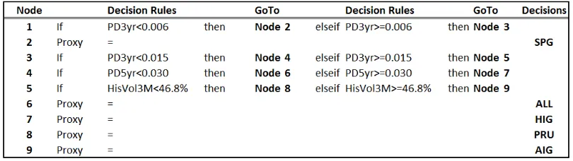
Table 2 shows the decision rules generated by the Decision Tree algorithm using as feature vector x:=(PD3yr,PD5yr, σh_3m), for the five observable counterparties indicated by their codes in the last

column of the table. The algorithm was run on data collected from the 100 days leading up to Lehman’s bankruptcy on 15-Sept-2008: see Appendix A.

The tree has nine nodes, labelled from 1 to 9. Depending on the values of its feature variables, a nonobservable will be led through a sequence of nodes starting from node 1, until ending up with a node associated with a single observable counterparty, to which it then is classified.

Table 2: A Simple Illustrative Example of Decision Tree based CDS Proxy Method

As shown in Table 1, we have investigated the impact of tree-size and of the different definitions of purity gain (Gini, Entropy, Twoing) on the Decision Tree’s classification performance: see section 3 for the Cross-classifier comparison, and Figure 18 and its associated table for the Intra-classifier comparison.

It is known that the Decision Tree algorithm may suffer from overfitting: it may perform well on a training set but fail to achieve satisfactory results on test sets. For that reason we have also investigated the so-calledBootstrapped Aggregated TreesorBagged Trees, an example of an Ensemble Classifier which we discuss in further detail in Section 2.9 below.

2.7

Support Vector Machines

Traditionally, the explanation of a SVM starts with the case of a two-class classification problem, with classes y = 1 and y = −_{1, for which the feature vector components of the training data}

DT _{= {(x}

i,yi) ∈ Rd× {±1},i = 1, . . . ,n}can belinearly separated in the sense that we can find a

hyperplaneH ⊂_Rn_{such that all datex}

ifor whichyi = 1 lie on one side of the hyperplane, and

those for whichyi=−1 lie on the other side. Needless to say, for a given data set, the assumption

of linear separability is not necessarily satisfied, and the case when it isn’t will be addressed below. If it does hold, one also speaks of the existence of ahard margin.

Assuming such a hard margin, the idea of a SVM is to choose a separating hyperplane which maximises the distances to both sets of feature variables, those for whichyi=1 and those for which

yi =−1.The two distances can be made equal, and their sumMis called themargin: see Figure

5. Using some elementary analytic geometry, this can be reformulated as a quadratic optimisation problem with linear inequality constraints:

        

minβ,β0||β||

2

subject to

yi

βT_x i+β0

≥₁,_i=₁, . . . ,n.

(19)

Data points for which the inequality constraint is an equality for the optimal solution are called

support vectors: these are the vectors which determine the optimal margin. If (β∗_{, β}∗

0) is the, unique,

optimal solution, the any new feature-vectorxis assigned to the classy=1 ory=−_{1 according to} whetherby(x) is positive or negative, where

by(x)=β

∗T_x+β∗

0. (20)

The bigger|

by(x)|the more ”secure” the assignation of the new data pointxto its respective class, a

point to keep in mind for the extension of the algorithm to multi-class classification below.

2.7.1 An illustration of Margin

Figure 5 illustrates the concept of linearly separable data with maximal marginM.

Figure 5: SVM Illustrative Example for Margin

2.7.2 Non-linearly separable data

If the feature data belonging to the two classes are not linearly separable, they can always be sepa-rated by some curved hyper-surfaceS, and the data become linearly separable in new coordinates (ξ1, . . . , ξd) in which for example the equation ofSreduces toξ1 =constant.A standard example

will become separable in polar coordinates. More generally, one can always find an invertible smooth mapϕfromRdinto someRk withk≥d such that the transformed feature-vectorsϕ(xi)

become linearly separable. One can then run the algorithm in Rk on the transformed data set

{₍ϕ_(xi),_{yi) :i}=₁, . . . ,_N}_{, and construct a decision function of the form}

by(x)=β

∗T_ϕ(x)+β∗

0 which

can be used for classification.

From a theoretical point of view this is very satisfactory, but from a practical point there remains the problem on how to let the machine automatically choose an appropriate mapϕ.To circumvent this we first consider the dual formulation of the original margin maximisation problem (19). It is not difficult to see that the optimal solution can be written as a linear combinationβ∗ =Pn

i=1α

∗

ixi

of the data points: any non-zero componentβ⊥ofβperpendicular to thexiwould play no r ˆole for

the constraints, but contribute a positive amount of||_β⊥||2_{to the objective function. In geometric}

terms, if all data lie in some lower-dimensional linear subspace (for example a hyperplane), then the optimal, margin-maximising, separating hyperplane will be perpendicular to this sub-space. One can therefore limit oneself toβ’s of the formβ=P

iαixi, and instead of (19) solve

          

minα,α0 P

i,jαiαjxT_jxi

s. t.

yi

_P

jαjxT_jxi+α0

≥₁, _i=₁, . . . ,n.

(21)

For the transformed problem we simply replace the inner productsxT_jxibyϕ(xj)Tϕ(xi): note that the

resulting quadratic minimisation problem is alwaysn-dimensional, irrespective of the dimensionk

of the target space ofϕ.Now the key observation is that the symmetricn×_{n-matrix with coe}ffi_cients

k(xi,xj)=ϕ(xj)Tϕ(xi) (22)

is positive definite3_{, and that, conversely, ifk(x,y) is any function for which the matrix} k(xi,xj)

i,j

is positive definite, then it can be written as (22) for an appropriateϕ, by a general result known as Mercer’s theorem. Functionskfor whichk(xi,xj)

i,jis always positive definite, whatever the

choice of points xi, are called positive definite kernels. Examples of such kernels include the

(non-normalised) Gaussiansk(x,y)=e−c||x−y||2

and the polynomial kernels1+yT_xp_{, wherepis a}

positive integer.

To construct a general non-linear SVM classifier, we choose a positive definite kernelk, and

solve _          

minα,α0 P

i,jαiαjk

xi,xj

s. t.

yi

_P

jαjk

xi,xj

+α0

≥₁, _i=₁, . . . ,n.

(23)

The trained classifier function then is the sign ofby(x), where

by(x) :=

n

X

j=1

α∗

jk

x,xj

+α∗

0,

the∗indicating the optimal solution.

2.7.3 Hard versus soft margin maximisation

Although linear separation is always possible after transformation of coordinates, it may be ad-vantageous to allow some of the data points to sit on the wrong side of the separating surface, if we do not want the latter to behave too ”wildly”: think of the example of two classes of points,

3_{meaning that for all vectors (v}

”squares” and ”circles”, with all the ”circles” at distance larger than 1 from 0, and all the ”squares” at distance less than 1, except for one, which is at distance 100.

Also, even if the data can be linearly separated, it may still be advantageous to let some of the data to be miss-classified, if this allows us to increase the margin, and thereby better classify future data points. We therefore might want to allow some miss-classification, but at a certain cost. This can be implemented by replacing the 1 in the right hand side in thei-th inequality constraints by 1−ξ_{i, adding a cost function C}P

iξi to the objective function which is to be minimised, and

minimising also over allξi≥0.

2.7.4 Multiclass classification

We have given the description of the SVM classifier for two classes, but we still have to explain how to deal with a multi-class classification problem where we have to classify a feature vectorx amongNclasses. There are two standard approaches to this: we can break up the problem intoN

two-class problems by classifying a feature vector as belonging to a given class or not belonging to it, for each of the classes. The two-class algorithm then provides us then withNclassifiers functionsbyj(x),j=1, . . . ,N, which we then use to construct a global classifier by taking the (or a)j

for whichbyj(x) has maximum value (maximum margin). The other approach is to construct SVM

classifiers for each of theN(N−₁₎/_{2 pairs of classes and again look select the one for which the} two-class decision function has maximal value.

As indicated in Table 1, we investigated the SVM algorithm with Linear, Gaussian and Polyno-mial kernel and tested their performance for our CDS-Proxy problem. The results are presented in Section 3 and Appendix B.

2.8

Neural Networks

2.8.1 Description

Motivated by certain biological models of the functioning of a human brain and of its constituting neurons, Neural Networks represent a learning process by a network of stylised (mathematical models of) single neurons, organised into an Input Layer, and Output Layer and one or more intermediate Hidden Layers. Each single ”neuron” transforms an input vectorz=(z1, . . . ,zp) into

a single outputuby first taking a linear combinationP

iwiziof the inputs, adding a constant or

bias termw0, and finally applying a non-linear transformation f to the result:

u= fXwizi+w0

= fwTz+w0

, (24)

where the weightswiof all of the neurones will be ”learned” through some global optimisation

procedure.

The original idea, for the so-calledperceptron, was to take for f a threshold function: f(x)=1 ifx ≥_{aand 0 otherwise, which would only transmit a signal if the a}ffi_{ne combination of input} signalswT_z+w

0was sufficiently strong. Nowadays one typically takes forfa smooth differentiable

function such as the sigmoid functionσdefined by

σ(x)= 1

1+e−cx (25)

neurons in a given Layer to all of the neurons in the next Layer. The outputsuf _=(uf

ν)νof the final Hidden Layer undergo a final affine transformation to giveKvalues

wT_kuf+wk0, k=1, . . . ,K. (26)

for certain weight vectors wk = (wkν)ν and bias terms wk0 which, similar to the weights of the

Hidden Layers, will have to be learned from test data: more on this below. For a regression with a Neural Network these would be the final output, but for a classification problem we perform a further transformation by defining

πk=

ewT ku

f_+w k0

PK

l=1ew

T

luf+wl0, (27)

The interpretation is thatπk, which is a function of the inputxas well as of the vectorWof all the

initial, intermediary, and final network weights, is the probability that the feature vectorxbelongs to classk.

To train the network we note that minus the log-likelihood that an input xi belongs to the

(observed) classyi∈ {1, . . . ,K}is

−

N

X

i=1

K

X

k=1

δyi,klogπk(xi;W), (28)

whereWis the vector of all the weights and biases of the network. This is also called the

cross-entropy. The weights are then determined so as to minimize this cross-cross-entropy. This minimum is numerically approximated using a gradient descent algorithm. The partial derivatives of the objective function which are needed for this can be computed by backward recursion using the chain rule: this is called the backpropagation algorithm: see for example Hastieet al. (2009) for further details.

The final decision rule, after training the Network, then is to assign a feature vectorxto that classkfor whichπk(x,c_W) is maximal, where the hat indicates the optimised weights.

2.8.2 An Illustrative Example of A Simple Neural Network

Figure 6shows a simple 3-Layer Neural Network including Input Layer (dfor # of features), one Hidden Layer (nfor # of Hidden Units) and Output Layer.

2.8.3 Parameterization

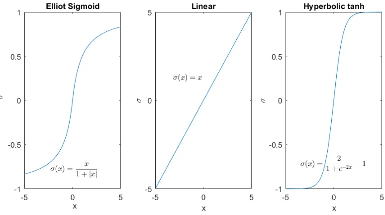
We restricted ourselves to Neural Networks with a single Hidden Layer, motivated by theuniversal approximation theorem of Cybenko and Hornik, which states that such networks are sufficient to uniformly approximate any continuous function on compact subsets of Rn. The remaining

relevant parameters are then the activation function f and the number of Hidden Units. As activation function we selected and compared the Elliot-sigmoid, purely linear and hyperbolic tangent functions: see Figure 7. We also investigated the impact of the number of Hidden Units on Classification performance: the greater the number of these, the more complex the Neural Network, and the better, one might na¨ıvely expect, the performance should be. However, we found that, depending on Feature Selection, the performances for our proxy problem quickly stabilise for a small number of hidden neurons: see Figure 20. We found the Neural Networks to be our best performing classifiers: see Section 3 for further discussion.

2.9

Ensemble Learning: Bagged Decision Trees

Figure 6: An Illustration for A Simple Neural Network

generates new training setsD1, . . . ,DB by uniform sampling with replacement, and uses these to

train classifiersby1(x), . . . ,byB(x).The final classification is then done bymajority vote (ordecision by committee): a feature vectorxis associated to the class which occurs most often amongst thebyi(x).

We will callBthe number oflearning cyclesof the bagging procedure.

Breiman (1996) found that bagging reduces variance and bias. Similarly, Friedman and Hall (2000) report that bagging reduces variance for non-linear estimators such as Decision Trees. Bagging can be done using the same classifier algorithm at each stage, but can also be used to combine the predictions of classifiers from different classifier families. In this paper we have limited ourselves to bagging Decision Trees, to address the strong dependence of the latter on the training set and its resulting sensitivity to noise.

2.9.1 An Example of Bagged Tree performance

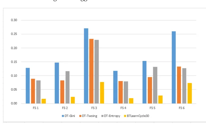
Figure 8 show the improvement in performance, in terms of misclassification rates, from using the Bagged Tree as compared to the ordinary Decision Tree, for all three types of impurity measures (Gini, Twoing and Entropy). For this graph, the number of Learning CyclesBwas set to 30. We also investigated the dependence of the accuracy onBand found that it stabilizes aroundB=30 for each of the Feature Selections: see Figure 21 and Section 3.2 for further discussion. After bagging, the Decision Tree algorithm rose from sixth to third best performing classifier family: cf. Section 3.1 below.

2.10

Statistical Procedures for Classifier Performance

To examine performance of the various classifiers, we used the well establishedK-fold Cross Vali-dationprocedure, which is widely used in Statistics and Machine Learning.

2.10.1 K-fold Cross Validation

LetDO_{be a set of observed data, consisting of feature vectors and the classes they belong to (for}

Figure 7: Activation Functions for Neural Network

1. Randomise4DO_{and split it as a union ofKdisjoint subsetsD} n(K):

DO=

K

[

n=1

Dn(K).

Typically, theDn(K) will be of equal size. ForStratified K-fold Cross Validation, each Dn(K)

is constructed in such a way that its composition, in terms of the relative numbers of class-specific samples which it contains, is similar to that ofDO_{.Stratified Cross Validation serves}

to limit sample bias in the next step.

2. Forn = 1,2, . . . ,K, define theholdout samplebyDHn =_D

n(K) and train the classifier on the

n-th Training Set defined by

DTn=_DO_−DHn. ₍₂₉₎

Letbyndenote the resulting classifier.

3. For each n, testbyn on the holdout sample D

Hn _{by calculating theMisclassification Rate} H

n

defined by

H

n =

1 #DHn

X

(x,y)∈DHn

1−_I(y,_yˆ(x)),

(30)

whereI(u,v)=1 ifu=vand 0 otherwise.

4. Take the sample mean and standard deviation of theH

n as empirical estimates for theExpected

Misclassification Rateand its standard deviation by :

b uK=

1

K

K

X

n=1

H n

b SK=

v t 1 K K X

n=1

(H

n −ubK)2. (31)

Figure 8: Bagged Trees vs A Decision Tree

If we assume a distribution for the sampling error, such as a normal, a Studenttdistribution, or even a Beta distribution (seeing that theεHn are all by construction between 0 and 1) we can translate

these numbers into a 95% confidence interval, but we have limited ourselves to simply reporting

buKandbSK. Also note that 1−buKwill be an estimate for theExpected Accuracy Rate.

2.10.2 Choice ofKforK-fold cross validation

Kohavi (1995) recommends using Stratified Cross Validation to test Classifiers. Based on extensive datasets, it suggests thatK =10 is a good choice. This was also found by Breiman et al. (1984), who r