The Development and Analysis of Beamforming Algorithms Used for Designing an Acoustic Camera

(1)

http://www.sciencepublishinggroup.com/j/ajese doi: 10.11648/j.ajese.20190304.15

ISSN: 2578-7985 (Print); ISSN: 2578-7993 (Online)

The Development and Analysis of Beamforming Algorithms

Used for Designing an Acoustic Camera

Sanja Grubesa

1, *

, Jasna Stamac

2

, Ivan Krizanic

2

, Antonio Petosic

1

Faculty of Electrical Engineering and Computing, University of Zagreb, Zagreb, Croatia 2_{Geolux d. o. o., Zagreb, Croatia}

Email address:

*

Corresponding author

To cite this article:

Sanja Grubesa, Jasna Stamac, Ivan Krizanic, Antonio Petosic. The Development and Analysis of Beamforming Algorithms Used for Designing an Acoustic Camera. American Journal of Environmental Science and Engineering. Special Issue: Smart Cities – Innovative Approaches. Vol. 3, No. 4, 2019, pp. 94-102. doi: 10.11648/j.ajese.20190304.15

Received: November 8, 2019; Accepted: November 29, 2019; Published: December 6, 2019

Abstract:

This paper discusses the beamforming algorithms used in developing an acoustic camera which can be used for the purpose of localizing sound sources. In order to design an acoustic camera which can display results in the form of an intensity map, it is necessary to determine the beamformed signal for all the desired incident angles, i.e. for all the desired pairs of azimuth and elevation angles. For the purpose of obtaining the beamformed signal required for localization of sound sources, two beamforming algorithms, which differ in the domain in which the beamforming is performed, were developed named respectively DASt.m and DASf.m. The aforementioned algorithms are implemented in the numerical computing environment MATLAB and furthermore compared in this paper. The beamforming was carried out using both of the aforementioned algorithms for all desired azimuth and elevation angle pairs and the obtained results were compared. In order to compare these two developed beamforming algorithms measurements were conducted in an open space using a Uniform Circular Array (UCA). The utilized UCA consists of 16 identical omnidirectional microphones which form a basic circular acoustic camera. The research showed that the DASf.m algorithm gives better results than the DASt.m algorithm, especially for the intensity maps of the average of the signal.

Keywords:

Beamforming, Delay and Sum Algorithm, Time Difference of Arrival, Acoustic Camera, Uniform Circular Array

1. Introduction

When speaking about the concept of smart cities, designing an efficient acoustic camera could present an innovative approach to noise monitoring and in addition to detection of uncommon sound sources (i.e. which could pose a certain risk or threat) in sound environments familiar to the residents. The acoustic camera is a microphone system consisting of a microphone array [1-4]. The spatial sound is recorded using a microphone array and a separate signal is generated for each microphone. Due to the geometric shift between the microphones, the sound reaches each microphone at a different time. The time delay between the signals recorded by the microphones in the array is referred to as Time Difference of Arrival – TDOA [5-7]. Adding the

delay to a particular microphone enables directivity pattern shifting. The formation of the directivity pattern, i.e. beamforming, is a type of signal processing which enables the localization of a sound source. One of the simplest beamforming algorithms is the Delay and Sum – DAS algorithm [8-10]. Using such an algorithm achieves the amplification of the sound coming from a certain direction and in addition, provides the reduction of noise and reflections coming from the space surrounding the array.

(2)

the signal delay is added. Both algorithms were implemented using MATLAB. The measurements were conducted in an open space using a 16-element uniform circular array (UCA) with a radius of 0.25 meters. Each of the array elements is a G.R.A.S. Type 40PH omnidirectional microphone [11]. A DJI Spark quadcopter was used as the recorded sound source [12].

2. Microphone Array

2.1. Time Difference of Arrival (TDOA)

Due to the difference in the distance the sound has to “travel” to reach each microphone in the array a time delay occurs between the signals that are being recorded by the microphones. This type of delay is named respectively Time Difference of Arrival (TDOA) and it can be utilized to localize the sound source. Adding the time delay to individual microphones in the array enables steering the directivity pattern in the desired direction. TDOA can be considered for two different cases; TDOA in a near field and TDOA in a far field. Whether the microphone array is located in the near or far field depends on the relative ratio between the distance from the sound source to the microphone array and the distance between adjacent microphones in the array.

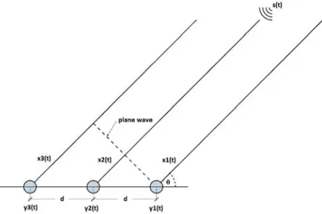
Figure 1. A linear microphone array in a far field.

Figure 2. A linear microphone array in a near field.

When the microphone array is located in the far field, as shown in Figure 1, the sound form the source is radiated as a plane wave meaning that the incident angle θ, with respect to the array axis, will be equal for every microphone in the array. The signal coming from the source is represented by s(t). The additional distance that the sound has to “travel” to reach the i-th microphone mi, with respect to the reference

microphone m1, equals to ∙ , where di is the distance

from the i-th microphone mi to the reference microphone m1.

In the case of a linear array the microphones in the array are positioned equidistantly, i.e. di = d, so that the distance to a

particular microphone in the array is equal to ∙ ∙ . For such linear array it is possible to define the time delay τi for

each one of the microphones mi. That time delay represents

the TDOA for a uniform linear array in the far field and it can be calculated with the following equation [8]:

(1)

where c is the speed of sound in air (i.e. c = 343 m/s). For every microphone mi of the uniform linear array a

signal is defined as:

. (2)

Each of the signals xi(t) can be represented by the phase

shift of the incoming signal:

(3)

!"# $ %&' (

) (4)

that is, for λ = c/f0:

!"$ %&' (

* . (5)

In case of more than one source, i.e. there are K sources, and each microphone in the array has its own noise, the total signal of the i-th microphone is equal to the sum of contributions of the signals from all K sources and the noise of that i-th microphone, ni(t):

∑,_-. !"$ %&' (* / 0 . (6) When the microphone array is located in the near field, as shown in Figure 2, the calculation becomes more complex as the incident angle for individual microphones is no longer the same, i.e. in the near field each microphone mihas its own

incident angle θk. From Figure 2 the distances r1 and r2 can

be calculated using the cosine rule:

122 1.2/ 2/ 21. cos . (7)

172 1.2/ 4 2/ 41. cos . (8) For a uniform linear array, the TDOAs in the near field are defined as:

(3)

.7 9; 9: (10)

The values of θ1, r1, r2 and r3 can be calculated by solving

the system of equations (7), (8), (9) and (10), where τ12 and

τ13 can be obtained through processing of the signals

recorded by the microphones in the array.

2.2. Beamforming

One of the most common and simplest beamforming algorithms is the Delay and Sum (DAS) algorithm (see Figure 3). The main idea upon which the algorithm is based is that the signals of individual microphones can be delayed by the calculated TDOA in order to obtain a constructive summation of the signals coming from the desired direction. The signals coming from other directions are out of phase and are therefore summed up destructively. Thus, the amplification of the signal from the desired direction, as well as attenuation of the signal from other directions, is achieved.

The DAS algorithm in the time domain can be divided into four phases:

1.Recording the sound source with the microphone array; 2.Determining the delay between the signals recorded by

each microphone in the array;

3.Calculating the delay of the signals with respect to the desired direction to ensure that the part of the desired signal has the same phase on all channels

4.Summation of signals on all channels and normalization of the sum with the number of microphones in the array. Ideally, the far field scenario, shown in Figure 1, and a narrowband signal is assumed. If all the microphones are identical, the sound intensities W on all the microphones should be virtually equal, given the distance between the microphones d is relatively small:

< = ∙ >, > 4@12_{→ < = ∙ 4@1}2_,₍₁₁₎

where I denote the intensity of a point source.

In the case of a known incident angle θ, the delay between the signals on individual microphones TDOA can be determined using equation (1). On the other hand, if the incident angle is unknown, the delay can be calculated using cross-correlation of the recorded signals. Cross-correlation of signals Rij is a measure of similarity of two signals as a

function of the time shift τ between them and can be calculated using equation (12). The maximum cross-correlation value is achieved when there is a maximum overlap of two signals. Considering that the processing is performed on a signal which is sampled at a specific sampling frequency fs, the cross-correlation should be

performed on a sampled signal as well.

B ∑, C C

-D (12)

The sampling frequency fs causes some limitations when

detecting the TDOA due to the spatial resolution of the system. The minimum distance dmin is defined as the distance

(13) at which the delay is equal to one sample.

E F _G_H (13)

Figure 3. DAS algorithm: amplification of the signal from the desired direction and attenuation of the signal from other directions [9].

In the DAS algorithm's third step, a delay is added to the signals recorded by each microphone in order that all of the signals have the same phase. The delayed signal of the i-th microphone is given by equations (14) and (15):

I J K L / M (14)

I / M , 1,2,3, … , Q (15)

In equations (14) and (15) wi represents the sound intensity

attenuation which occurs as a result of sound propagation, whereas s(t) represents the sound source signal, and τi(θ)

denotes the delay of the signal recorded by the i-th microphone with respect to the location of the sound source. Furthermore, vi(t) indicates the noise of the i-th microphone,

and t denotes time. Combination of equations (14) and (15) yields the equation for the total output signal:

I _R.∑ IR

-D _R.∑ KR-D / M L (16)

In equation (16) the sum of all microphone output signals is divided by the number of microphones in the linear array giving the normalized signal value, i.e. the signal value that is approximately equal to the signal emitted by the sound source. Modifying equation (16) generates the equation for the total output signal in decibels:

I S 20 log.D_R.∑

!"# $%&' ( )

R .

-D (17)

In case of a uniform circular array, shown in Figure 4, the signal recorded by a certain microphone is given by the following equation:

WE _2X. Y Z [\]_] K ^

_`

)a b cd !"ef \ cd b cd cd!"ef gL [ (18)

(4)

Figure 4. Plane wave impinging on a uniform circular array with M sensor [13].

By organizing equation (18), equation (19) is obtained.

WE _2X. Y Z [ K ^

_`

)∙ cd a!"ef bgL

\]

] [ (19)

Following the methodology in the case of the linear array, the total output signal of a uniform circular array is calculated as the sum of signals from all M microphones:

I _2X.Y Z [ ∙_R.∑R . K ^ _`₎∙ cd a!"e_f bgL

-D [

\]

] (20)

Same as in the case of a linear array, the circular array can be steered in any direction. Time delay τm which is calculated

for each microphone before the summation of signals is given as follows:

E hacos i sin cos2XE_R / sin i sin sin2XE_R g (21)

while the total output signal is equal to the normalized sum of signals from all M microphones:

l _R.∑R .E-DWE / E (22)

3. Beamforming by Means of Developed

Algorithms

Figure 5. A uniform circular array with 16 G.R.A.S. Type 40PH omnidirectional microphones.

The measurements were performed using a 16-element uniform circular array with a radius equal to 0.25 meters, as shown in Figure 5. Each of the array elements is a G.R.A.S. Type 40PH omnidirectional microphone. Data acquisition was carried out using a National Instruments device NI

cDAQ-9174 with four associated NI 9234 circuits, shown in Figure 6 [14]. Such device is used to discretize continuous signals, thereby converting them from analogue to digital form suitable for further analysis and processing. Analysis and processing of acquired signals was performed using MATLAB. For the purpose of beamforming, two algorithms were developed, named respectively DASt.m and DASf.m.

Figure 6. National Instruments device NI cDAQ-9174 with 4 associated NI 9234 circuits.

In order for the results to be displayed in the form of an intensity map, it is necessary to determine the beamformed signal for all the desired incident angles. The beamformed signal is obtained using one of the beamforming algorithms, DASt.m or DASf.m. The beamforming was performed for angles i m K 45,45L and m K 45,45L, where φ and θ are the desired azimuth and elevation angles respectively. For each of the microphones in the array a delay (23) was calculated for every observed point in space, i.e. for each azimuth and elevation angle pair.

E h asin cos 2XE_R i g (23)

The value of the delay for a certain point in space refers to the delay of a particular microphone with respect to the centre of the microphone array. Hence the delay will be negative if, for a specific pair of azimuth and elevation angles, the signal reaches a microphone before it reaches the array centre. Likewise, the delay will be positive if the signal reaches the array centre first. For all of the recorded signals a comparison of the results was made using the two developed algorithms, DASt.m and DASf.m.

3.1. The DASt.m Algorithm

(5)

to determine the coefficients of the FIR filter. The desired window can be chosen within the algorithm. The algorithm cannot process negative delay values and therefore all the delays need to be additionally shifted so that the delay with the smallest, i.e. most negative, value becomes the reference value. The output of the algorithm is the normalized sum of all delayed signals.

3.2. The DASf.m Algorithm

The DASf.m algorithm adds the delay to the signals in the frequency domain. The zero-padded Fast Fourier Transformation (FFT) [15] of the signal recorded by the microphones is multiplied by a frequency domain delay function which is shown with equation (24). The output of the algorithm is once again the normalized sum of all delayed signals.

e 2XG e₍₂₄₎

Adding the delay in the frequency domain will result with more accurate results than delaying the signals in the time domain, however the frequency domain computation is significantly slower due to its complexity.

3.3. Algorithm Comparison Results

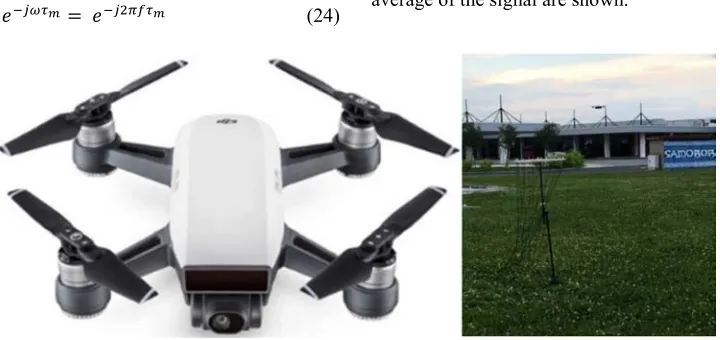
Table 1 provides a comparison of the results obtained using algorithms DASt.m and DASf.m. The intensity maps were made for a recording of a DJI Spark quadcopter, shown in Figure 7. The quadcopter was recorded using the previously described 16-element uniform circular array. Table 1 shows the intensity maps for two seconds of the recorded signal, with a division of the total signal into 200 milliseconds duration segments. For every 200 milliseconds duration segment, intensity maps for the maximum and the average of the signal are shown.

Figure 7. DJI Spark quadcopter.

Table 1 shows that the DASf.m gives better results than the DASt.m algorithm, especially for the intensity maps of the average of the signal. It took 8 seconds to process one 200 milliseconds segment of the signal recorded with all 16 microphones using the DASt.m algorithm, therefore the processing of the 2 second duration signal, divided into 200 milliseconds duration segments, required 1.38 minutes. Using the DASf.m algorithm the required run times increased

to 55 seconds for 200 milliseconds of the signal, and 9.23 minutes for the 2 seconds of the signal divided into 200 milliseconds segments. In our future work, the implementation of this algorithm in a Field-programmable Gate Array (FPGA) circuit is planned which will speed up the process and enable real-time analysis. It was therefore decided that the frequency domain beamforming will be used as this will produce more accurate results.

Table 1. The comparison of the results obtained using algorithms DASt.m and DASf.m.

Duration segments (ms)

DASt.m DASf.m

Maximum Average Maximum Average

0 - 200

(6)

Duration segments (ms)

DASt.m DASf.m

400 - 600

600 - 800

800 - 1000

1000 - 1200

1200 - 1400

1400 - 1600

1600 - 1800

(7)

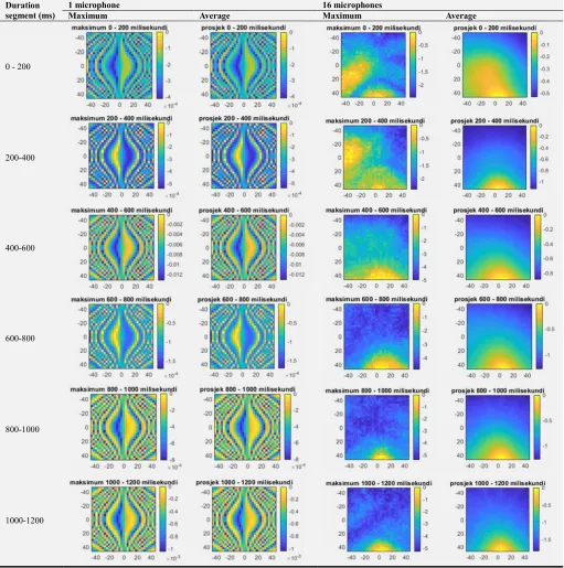
Table 2 provides a comparison of the intensity maps of the signal maximum and signal average recorded with a single microphone of the array and with all 16 microphones of the array. The beamforming was performed in the frequency domain using the DASf.m algorithm. Once more, the same 2 seconds of the signal were divided into 200 milliseconds duration segments shown in Table 1.

In addition, Table 2 shows that it is impossible to determine the position of the sound source using a single microphone, while using all the microphones of the circular array makes it possible to establish the location of the source either on the intensity map of the signal maximum or the intensity map of the signal average, and in the majority of cases the position is clearly visible on both intensity maps.

Table 2. Comparison of intensity maps of the maximum and average of the signal obtained using one microphone and all 16 microphones.

Duration segment (ms)

1 microphone 16 microphones

0 - 200

200-400

400-600

600-800

800-1000

(8)

1200- 1400

1400- 1600

1600- 1800

1800- 2000

4. Conclusions

The research presented in this paper showed that when designing an acoustic camera, one should follow the described procedure which contains several steps. One of the steps is to develop and test a beamforming algorithm for displaying results in the form of an intensity map. The main idea when using the Delay and Sum (DAS) algorithm is that the signals of individual microphones can be delayed by the calculated TDOA in order to obtain a constructive summation of the signals coming from the desired direction.

In our research two different beamforming algorithms DASf.m and DASt.m implemented in MATLAB were compared. The measurements were conducted in an open space using a 16-element Uniform Circular Array (UCA) i.e. in this paper a basic circular acoustic camera was used for conducting measurements. The research showed that DASf.m gives better results than the DASt.m algorithm, especially for the intensity maps of the signal average. Furthermore, results showed that it is impossible to determine the position of the sound source using a single microphone, while using all the microphones of the circular array makes it possible to determine the location of the source either on the intensity map of the signal maximum or the intensity map of the signal average. We denote that in most cases the position is clearly visible on both types of intensity maps.

The future work will be oriented on the implementation of the aforementioned beamforming algorithm in a

Field-programmable Gate Array (FPGA) which will accelerate the process while enabling real-time analysis. This designed algorithm will be used in a prototype of an acoustic camera with Micro-electromechanical Systems (MEMS) microphones.

The research provided in this paper could serve as a powerful instrument in the concept of smart cities in terms of innovative approach to noise monitoring in urban areas. In addition, an efficient and appropriate acoustic camera could serve as a tool for detection of unfamiliar sound sources which could pose a certain risk or treat in acoustic environments which are familiar to the majority of urban residents.

Acknowledgements

This work has been supported by the European Union from European regional development fund (ERDF) under the project number KK.01.2.1.01.0103 Acoustical Camera (in Croatian: Akustička kamera).

References

[1] J. Grythe, Acoustic camera and beampattern, Technical Note Norsonic, Oslo, Norway, 2015.

(9)

[3] B. Zimmermann and C. Studer, FPGA-based Real-Time Acoustic Camera Prototype, Proc. of IEEE Int. Symp. on Circuits and Systems (ISCAS), Paris, France, 2010.

[4] J. Stamac, S. Grubesaand A. Petosic, “Designing the Acoustic Camera using MATLAB with respect to different types of microphone arrays”, Second International Colloquium on Smart Grid Metrology, SMAGRIMET 2019.

[5] M. Brandstein and D. Ward, Microphone Arrays: Signal Processing Techniques and Applications, Digital Signal Processing. Springer, 2001.

[6] T. E. Tuncer and B. Friedlander, Classical and Modern Direction-of-Arrival Estimation, Academic Press, 2009. [7] E. T. Roig, Elisabet, Beamforming Techniques for

Environmental Noise, Brüel & Kjær, 2009.

[8] J. Benesty, J. Cheng and Y. Huang, Microphone Array Signal Processing, Springer-Verlang, 2008.

[9] http://www.labbookpages.co.uk/audio/beamforming/delaySum .html

[10] B. D. Van Veen and K. M. Buckley, Beamforming: A versatile approach to spatial filtering, IEEE ASSP Mag., 5 (2), 1988. [11]

https://www.gras.dk/products/special-microphone/array-microphones/product/178-40ph [12] https://www.dji.com/hr/spark

[13] N. Wu, Z. Qu, W. Si, and S. Jiao, DOA and Polarization Estimation Using an Electromagnetic Vector Sensor Uniform Circular Array Based on the ESPRIT Algorithm, settings, Sensors, 16 (12), 2016.

[14] National Instruments device cDAQ-9174 http://www.ni.com/en-rs/support/model.cdaq-9174.html [15] S. W. Smith, The Scientist and Engineer's Guide to Digital