Crowdsensed Data Learning-Driven Prediction of
Local Businesses Attractiveness in Smart Cities
Andrea Capponi
], Piergiorgio Vitello
], Claudio Fiandrino
?, Guido Cantelmo
†,
Dzmitry Kliazovich
, Ulrich Sorger
], Pascal Bouvry
]]FSTC/CSC & SnT, University of Luxembourg, Luxembourg
,
?IMDEA Networks Institute, Madrid, Spain,
† Technical University of Munich (TUM), Germany
,
ExaMotive, LuxembourgE-mails:]{firstname.lastname}@uni.lu
,
?claudio.fiandrino@imdea.org,†g.cantelmo@tum.de,kliazovich@ieee.orgAbstract—Urban planning typically relies on experience-based solutions and traditional methodologies to face urbanization issues and investigate the complex dynamics of cities. Recently, novel data-driven approaches in urban computing have emerged for researchers and companies. They aim to address historical urbanization issues by exploiting sensing data gathered by mobile devices under the so-called mobile crowdsensing (MCS) paradigm. This work shows how to exploit sensing data to improve traditionally experience-based approaches for urban de-cisions. In particular, we apply widely known Machine Learning (ML) techniques to achieve highly accurate results in predicting categories of local businesses (LBs) (e.g., bars, restaurants), and their attractiveness in terms of classes of temporal demands (e.g., nightlife, business hours). The performance evaluation is conducted in Luxembourg city and the city of Munich with publicly available crowdsensed datasets. The results highlight that our approach does not only achieve high accuracy, but it also unveils important hidden features of the interaction of citizens and LBs.
I. INTRODUCTION
For decades, urban planners and researchers have relied on experience-based strategies and traditional methodologies to tackle urbanization issues. Nowadays, the pervasiveness of mobile devices permits to use Information and Communications Technology (ICT) by unleashing unprecedented possibilities in urban environments to improve citizens’ quality of life [1] and services, such as public lighting [2]. Citizens carrying smart devices are a potential data source according to the mobile crowdsensing (MCS) paradigm [3], [4]. The crowd market is projected to raise from USD 385.1 Million of 2016 to USD
1 142.5 Million by 2021 at a compound annual growth rate
of 24.31. Incentives and energy-efficient schemes are typically
employed to make MCS systems effective [5].
LBs require their owners (e.g., companies, individuals, and institutions) to take decisions for profit maximization and to offer competitive services to customers. The most crucial decisions include the typology of a LB and its location when opening, but also setting prices, the number of required employees per hour, and opening hours for proper management. Effective strategies to boost LBs require knowledge of the complex dynamics of urban environments, which depend on the spatial distribution of citizens and locations [6]. For instance, understanding real-time citizens’ mobility as well as forecasting significant flows of citizens moving to a specific urban area for a special event help municipalities to manage crowds and entrepreneurs in deciding suitable locations and required staff. To develop solutions for smart mobility [7], testbeds
1https://www.marketsandmarkets.com/PressReleases/crowd-analytics.asp
are prohibitively costly and relying on simulators to model pedestrian trajectories and crowdsensing activities [8] is a valid cost-effective alternative.
Traditional approaches to investigate LBs popularity rely either on surveys that capture users’ preferences or cellular traces that infer urban mobility [9]. However, such approaches are prone to users misbehavior, technical limitations (e.g., poor network coverage), and datasets available only from network operators [10]. Crowdsensed data-driven approaches may provide novel solutions in this direction by exploiting MCS systems and services like Google Maps that make available accurate information on travel times and popularity of LBs.
This work aims to bring one step further the research on urban computing and to boost LBs popularity by overcoming the limitations of historically experience-driven approaches. We leverage crowdsensed data to enforce highly-accurate classifi-cation of LBs category and attractiveness with ML techniques that are powerful to handle massive data volumes and widely employed from a variety of applications, such as to infer and predict human mobility in urban context [11]. In this work, we show that typical urban metrics (e.g., the centrality of places in street networks) fail to properly classify LBs, while combining crowdsensed data (e.g., peak hours in LBs) with basic ML techniques supports and improves typical experience-driven approaches. To illustrate with few representative examples, restaurants and pubs usually concentrate in close areas and influence one with each other, while LBs like pharmacies are uniformly distributed over a city. Also, reachability by public transport significantly impacts on LBs popularity.
II. BACKGROUND
A. Related works
Crowdsensed data-driven approaches can be applied to better tackle urbanization issues and understand citizens mobility [15]. In this context, MCS permits to directly gather data from users and infer their mobility patterns with high accuracy, e.g., classify residents and visitors and identify special events [16]. By feeding ML techniques with crowdsensed data can open up unexplored solutions. ML approaches are extensively used to extract information from large datasets acquired from various sources [17]. ML and deep learning models were applied to various areas, such as speech or image recognition, and in urban scenarios to detect accident risks [18] and predict traffic flows [19]. The use of learning techniques over crowdsensed data has become a win-win solution in different domains, such as to predict human judgments of pairwise image comparisons and produce urban perception at large scale [20]. Unlike the above proposals, this work aims to provide predictions of the popularity of LBs inferred by studying human mobility in urban environments. The closest work to our is [21] that has the objective of predicting the temporal dynamics of newly
established LBs by exploiting the check-in data of Foursquare
users. By contrast, we study generic LBs and rely on Google Popular Times data.
B. Crowdsensed datasets
Mobile users have at disposal several ways to share data such as location-based social networks (LBSN) (e.g., Facebook, Foursquare, Twitter, etc.), and crowdsourced applications (e.g., OpenStreetMap, Waze). Such contribution has made available large datasets that enable an analysis of citizens mobility, travel behaviors, accessibility of urban areas and popularity of LBs. In particular, Google makes available anonymized crowdsensed data passively collected from Google Maps users who opted into Google Location History2. These datasets include information on customers visits to LBs, such as popular times per hour, the average duration of visits, queuing time to access a service, and real-time popularity.
In this work, we exploit Google Popular Times with a twofold purpose. First, we investigate features that can influence the popularity of LBs. Second, we feed ML techniques on such dataset to classify category and attractiveness of LBs according to the considered features.
III. PRELIMINARYANALYSIS
This Section grounds the roots of our work by showing why traditional urban metrics fail to classify and predict LBs attractiveness properly.
Weekly popularity:Google Popular Times define the temporal
profile of a LB as a vector of normalized per-hour weekly values in the range [0 : 100]. In particular, 0 defines closing hours,1
the lowest amount of visits per-hour in a week, and 100the
highest. The use of normalized values permits to analyze the trend of LBs during a week and its influencing factors (e.g., LBs that have more success at weekends in touristic areas or at lunchtime in business districts). This hides the degree
2https://support.google.com/business/answer/2721884
0 20 40 60 80 100 120 140
0 20 40 60 80 100
Weekly hour (Mon-Sat)
Popular
Times
(%)
Average Rest-1 Rest-2 Rest-3 Rest-4 Rest-5 Rest-6 Rest-7 Rest-8 Rest-9
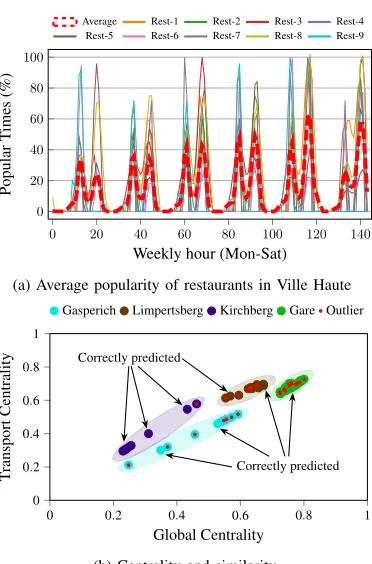
(a) Average popularity of restaurants in Ville Haute
0 0.2 0.4 0.6 0.8 1
0 0.2 0.4 0.6 0.8 1
Correctly predicted Correctly predicted
Global Centrality
Transport
Centrality
Gasperich Limpertsberg Kirchberg Gare Outlier
(b) Centrality and similarity
Fig. 1. Data aggregated from different Luxembourg districts for restaurants
of success of a single LB (e.g., having more customers than others), which is however not the purpose of this work.
Fig. 1(a) presents Popular Times of nine restaurants and their average from Monday to Saturday in Luxembourg city (Ville Haute), a district with offices (banks, public institutions), shops, tourists spots and places for nightlife (bars, pubs). Sunday is excluded because no information was available in the dataset. The peaks of popularity approximately at12,20,36,44, etc.,
correspond to lunch (12 PM) and dinner (8 PM) times of each day. Analyzing the peaks in pairs, we can compare the trend of restaurants day by day and understand the lifestyle of the district. During weekdays the peaks are around lunch time or equally spread at lunch-dinner time (restaurants full of workers) while on Saturday at dinner time because most offices are closed. Friday is the most popular day at both lunch and dinner times because both workers, tourists, and citizens populate restaurants.
Centrality and similarity:The popularity of LBs depends on
their proximity with other LBs and accessibility through public transportation. The centrality metric defines the importance of individual nodes in a network and can quantify popularity. Specifically, we consider thecloseness centrality, defined as
the sum of the length of the shortest paths between a node and all other nodes within the street network. We measure
global-centralityandtransport-centrality. Theglobal-centrality
defines the proximity of a LB with all other LBs:
CB(k) =
NB−1
P
i6=kdki
, (1)
where kis the k-th node,NB is the total number of LBs and
dki is the distance between a couple of nodes. The
transport facilities:
CT(k) =
NT
P
i6=kdki
, (2)
whereNT is the total number of transportation access points
(e.g., bus stops or metro stations) and dki is the distance
between the considered LB and a transport node. Considering the Earth as an oblate ellipsoid, the distance is computed with the shortest geodesic path [22]. While popularity measured with centrality identifies time-invariant characteristics of a LB, the
similaritycompares two LBs temporal profiles. The similarity
aims to correlate LB weekly popularity to the average of all LBs in the same district. To measure similarity, we exploit the symmetric index of Jensen-Shannon divergence (JSD) that outperforms the asymmetric Kullback-Leibler divergence (KLD) [21]. The similarity of two LBsiandj is:
J(Di, Dj) =H
Di+Dj
2
−H(Di) +2H(Dj), (3) where H is the Shannon entropy, D is the temporal profile of a LB, and J represents the divergence of two temporal profiles, The similarity can assume values in the range [0−1]. 0represents the maximum similarity (e.g., the temporal pattern
of a shop with itself) and1represents the maximum divergence.
Fig. 1(b) links centrality and similarity metrics in Lux-embourg city. The clusters represent four districts, in line with global- and transport-centrality of restaurants. Red dots represent LBs whose weekly temporal demand is closer to the average of other districts (outliers). On the contrary, dots of the same dominant color have a weekly pattern more similar to their geographical district. With the sole exception of Kirchberg district, most of the LBs are marked as outliers. Therefore, this analysis unveils that centrality and similarity are not enough to assess the popularity of LBs and their relationship with districts. The analysis correctly predicts the popularity of LBs in Kirchberg because the district is geographically separate from other districts of the city and it is home of European agencies, insurance and financial companies making the LBs in the area to share peculiar popularity trends. This paper shows how to overcome this shortcoming by enforcing a ML-based analysis of the same dataset.
IV. ML-AUGMENTEDMETHODOLOGY
This Section describes the methodology for applying ML techniques to crowdsensed data. The Popular Times datasets undergo a procedure to extract features and determine the most suitable inputs to train the ML algorithms. We select only the features that augment the output accuracy after the training phase, while the others are discarded. For space reasons, we omit this preliminary selection. Next (§ IV-A), we introduce the ML algorithms. Then (§ IV-B), we discuss the considered multi-classification problems, extracted input features, and output classes. Each output is classified by exploiting a one-vs-all approach. For each LB, the element corresponding to the predicted class is set to one, all others to zero.
A. Machine Learning Techniques
This study considers Support Vector Machine (SVM) with a Gaussian kernel and MultiLayer Perceptron (MLP) neural
network techniques for multi-classification problems. The choice is due to characteristics of our study, which presents a small number of features N (e.g., 1 −1 000), and an
intermediate number ofM training samples (e.g.,1−50 000).
The chosen ML approaches perfectly fit this scenario. Similar ML techniques like logistic regression or SVM without kernel (or linear kernel) have not been considered because they perform better whenN is relatively large if compared toM (e.g., 10 000and M between 1 and 1 000). In the following,
we briefly analyze the considered ML techniques.
Support Vector Machines (SVMs) aim to classify input
samples into output classes by dividing a hyperplane with an optimal boundary through kernel methods. To this end, it is crucial to perform fine tuning of the regularization parameter, typically named C. Furthermore, employing a kernel based on a gaussian function, it is required to set the standard deviation, indicated asγ.Ctrade-offs the correct classification of training samples and the smooth decision boundary. Small values lead to simple decision functions, which correspond to a higher tolerance to errors and smooth the classification on the training dataset. On the contrary, high values correspond to a classification with minimal error and a hyperplane with a small margin. Intuitively, γ defines how a single training sample influences other points according to its distance from the boundary.
Multilayer Perceptron (MLP)is a feedforward artificial neural
network that takes a vector as input and maps it into another vector as output. It is based on different hidden layers that connect inputs to outputs. Each layer includes a certain number of nodes and nodes of different layers are connected by links with different weights. The output of a node at each layer is given by the weighted sum of all inputs. Each node in the hidden layers is connected to all nodes of next and previous layers for a fully connected topology.
B. Predicting LBs Category and Attractiveness
We formulate two multi-classification problems to predict LBs category and attractiveness by feeding ML techniques with input features extracted from crowdsensed data.
Extracted features:After a preliminary analysis that we omit
for space reasons, we select as input features from the large available datasets those that performed better and we categorize them as intrinsicand extrinsic. Intrinsic features are given by
geo-location characteristics and owners’ decisions, which do not present a high variability over time (e.g., opening hours and type of service offered). These properties are already widely exploited in traditional approaches for urban analytics. Extrinsic features depend on the temporal interactions of citizens with LBs, such as waiting time and average time of staying. They change more rapidly than the intrinsic ones and depend on several factors, e.g., special events, time of day, day of the week, etc. The intrinsic features we consider
areglobal-centrality,transport-centrality,opening hours, and
category. The parameters that define centrality have already
been discussed in Sec. III.Opening hoursconsists of an array of
each hour in a weekday, the value0indicates closing time and
1opening time. The category depends on the service offered by
LBs. The extrinsic features are popular times,average time of
visit, and average waiting time. Popular times were discussed
in Sec. III. The average remaining time defines in minutes the duration of customers’ visits. The average waiting time indicates the minutes while waiting to access the service.
Output classes: LB categories depend on the service offered
by a LB. Output classes are public,store,health,restaurant,
and bar. The class public indicates generic services and
offices for the community, such as institutions, post, financial and insurance companies. Store includes each kind of shop
or seller for any goods, such as supermarkets, clothing, bakeries, etc.Healthcomprises public and private places related
to healthcare, e.g., hospitals, medical centers, dentists, and specialists. Restaurant includes all LBs that prepare meals
with seating places.Barconsists of LBs selling mainly drinks,
but can also include meals, e.g., pubs.
LB attractiveness is classified into working,nightlife,
week-end,business hours(Bus. H.), andshopping hours (Shop. H.).
Workingindicates LBs with peak hours during break times of
working areas, such as weekdays at mid-morning and lunchtime. It comprises typically shopping malls, bars, fast foods and some types of restaurants. The class nightlife shows peak
hours at dinner times during all week and overall on weekends, including restaurants, pubs, and clubs. Weekend describes low
popularity on weekdays and peak hours at weekends, which is typical of shopping malls located far from working areas and touristic places.Business hoursindicates typical opening times
and consequent popular hours of public offices, from early morning to mid-afternoon including lunch breaks. Shopping
hoursinclude the typical popularity hours of shops for different
goods, presenting a uniform distribution on both weekdays and weekends during daytime.
V. DATA-DRIVENEVALUATION
This Section first presents simulation set-up and performance metrics, then the obtained results.
A. Setting
To conduct the evaluation, we employ publicly available Popular Times of LBs for Luxembourg city and the city of Munich downloaded between July 21st and July 30th, 2018. These two cities present different characteristics in terms of morphology, size, street topology, and lifestyles of residents and visitors. This permits to conduct an effective analysis and discussion of the obtained performance. The datasets include1 084and3 784LBs for Luxembourg city and Munich respectively and are proportionally divided in 80%,10%, and
10%for training, cross-validation, and test phases respectively. The performance evaluation exploits Scikit-learn, which is a Python-based open-source library.
To predict the LBs category, the input features are:average
opening hours, time spent, global-, and transport-centrality.
In this case, we restrict the datasets to the LBs for which information on time spent is available (800 and1 600 LBs for
Luxembourg city and Munich respectively). The hyperparam-eters in the SVM approach are set toC= 28 andγ= 2−12.
We will further discuss the rationale about the selection of parameters (see discussion Fig. 3a). In the MLP approach, an exhaustive search with a grid-search algorithm leads to the choice of one hidden layer with13 nodes.
For LBs attractiveness, the considered features are opening
hours,category,district,popular times,global-, and
transport-centrality. In this case, the entire datasets were employed. The
methodology followed to set the hyperparameters is as for the LBs category. For SVM, the parameters areC= 26 and
γ= 2−10 (likewise above, the rational is discussed in Fig. 3b),
MLP consists of8 nodes per layer with2 hidden layers.
B. Performance Metrics
We consider precision, recall, F1 score, and accuracy indexes. While precision, recall, and F1 score are per-class measures, the accuracy averages the measures of all the classes. For completeness of the analysis, we consider i)true positive (tp)
andtrue negative(tn) values to indicate respectively acorrect
prediction of positive or negative class; (ii)false positive(f p)
andfalse negative(f n) values to denote anincorrectprediction.
In this context, a positive observation indicates the class under analysis, while a negative observation indicates all the other classes, according to the one-vs-all approach.
The precision indicates the ratio of correct positive
predictions over the total predicted positive occurrences
(tp/(tp+f p)). In other words, it indicates the capacity of the model tonotpredict another true class as the actual class. The
recallis the ratio of correct predictions on positive observations
to all the occurrences in class under analysis(tp/(tp+f n)). It indicates the capability of the model to catch all the samples of a class. TheF1 scoreis the weighted average of precision
and recall indexes and analyzes incorrect predictions. Typically, the F1 score is very useful to unveil insights from results when false positives and false negatives have different costs. The
accuracyis computed as the ratio of correct predictions over the
total occurrences and defines the performance of a classifier. Specifically, accuracy is the optimal performance indicator when the classes are symmetric, i.e., incorrect predictions have the same weights.
C. Results
TABLE I
STATISTICS FORLBCATEGORY AND ATTRACTIVENESS PREDICTION
PRECISION RECALL F1SCORE ACCURACY
SVM MLP SVM MLP SVM MLP SVM MLP Lux Mun Lux Mun Lux Mun Lux Mun Lux Mun Lux Mun Lux Mun Lux Mun Public 0.67 0.60 1.00 0.67 0.40 0.75 0.40 0.50 0.50 0.67 0.57 0.57
0.84 0.81 0.81 0.76
C
A
T
E
G
O
R
Y Store 0.82 0.88 0.81 0.87 0.95 0.92 0.89 0.91 0.88 0.90 0.85 0.89
Health 1.00 0.75 0.75 0.67 0.40 0.92 0.60 0.92 0.57 0.83 0.67 0.77
Restaurant 0.93 0.79 0.90 0.77 0.93 0.87 0.88 0.79 0.93 0.83 0.89 0.78
Bar 0.60 0.80 0.45 0.60 0.75 0.53 0.62 0.47 0.67 0.63 0.53 0.53
Average 0.85 0.81 0.83 0.75 0.84 0.81 0.81 0.76 0.84 0.80 0.81 0.75
A
T
T
R
A
C
T
IV
E
N
E
S
S Working 0.85 0.60 1.00 0.57 0.58 0.60 0.40 0.40 0.69 0.60 0.57 0.47
0.84 0.87 0.80 0.88 Nightlife 0.60 0.88 0.81 0.86 0.75 0.73 0.89 0.77 0.67 0.80 0.85 0.81
Weekend 0.80 0.71 0.75 0.79 1.00 0.67 0.60 0.73 0.89 0.69 0.67 0.76
Business hours 0.93 0.96 0.90 0.96 0.96 0.97 0.88 0.97 0.94 0.97 0.89 0.97
Shopping hours 0.80 0.81 0.45 0.81 0.80 0.91 0.62 0.92 0.80 0.86 0.53 0.86
Average 0.85 0.87 0.83 0.87 0.84 0.87 0.81 0.87 0.84 0.87 0.81 0.87
or working areas). For example, restaurants present higher values of precision in Luxembourg city because the opening hours are not as international as in a larger city like Munich, while bars are predicted with higher precision in Munich. In Luxembourg city, bars and restaurants share opening hours while in Munich pubs and clubs open until late night, unlike restaurants. Regarding the attractiveness, on the one hand, the class working is predicted with much higher precision in Luxembourg. The reason is as follows: LBs with peak visits during job breaks are typically not popular, i.e., receive lower visits during other moments of the day or with another type of customers (e.g., tourists at the weekend). On the other hand, the class working is not well predicted in Munich because LBs are popular at different times during the day with no distinctive working areas. Business and shopping hours present higher values in Munich because of its urban plan characterized by LBs concentrated in specific districts with easily recognizable peak hours (e.g., the city center and shopping malls). For similar reasons, note that the model catches most samples of class (recall index) for restaurants and stores with both cities and both techniques when predicting the category, and business and shopping hours when predicting the attractiveness. F1 score analyzes the incorrect predictions by presenting a weighted average of recall and precision and the results are in line with previous considerations.
To simplify understanding, Fig. 2 depicts confusion matrices to highlight single occurrences for each true and predicted class and summarizes the prediction results. Each cell contains a value that indicates the number of occurrences of a predicted class when testing true inputs. The colors in legend bars represent the percentage of correct predicted occurrences over the total of true class values, which corresponds to the recall index between 0 and 1. The columns show predicted class
values. The sum of all values in each row indicates the total occurrences for such class. The occurrences of correct predictions for each class are in the diagonal. The accuracy is the sum of all elements on the diagonal on all elements of the matrix. The analysis on the confusion matrices allows
to i) discuss and compare behaviors of different LBs and ii) extend the discussion in point i) to different cities. As expected and already pointed out in Table I, categories with distinctive features present a better prediction. The results in the table, however, do not show the wrong occurrences as confusion matrices allow. The categories restaurant and store achieve
higher recall for both ML techniques in both cities because LBs in these categories share distinctive characteristics like
opening hours. On the opposite, publicandbarhave a lower
recall, and their wrong predictions occur respectively instore
and restaurant. These LBs offer services with similar daily
patterns, e.g., stores - public offices, and bars - restaurants. Fig. 2(a) and Fig. 2(b) clearly highlight these considerations because in Luxembourg city 2 bars over 8 are predicted as restaurants whereas for Munich this occurs for14LBs over34. Note that the healthcategory achieves significantly different
results in the two cities. The motivation is the different number of LBs in the available datasets. In this case, higher precision is attributed to a larger dataset.
When analyzing the attractiveness, Fig. 2(c) and Fig. 2(d) unveil that the highest number of prediction errors occur for
working and nightlife classes. As previously discussed, the
motivation is that restaurants and bars exhibit a high popularity at lunch and dinner times, which are typical characteristics shared between working and nightlife classes. For instance,
Fig. 2(c) and Fig. 2(d) respectively show that in4 occurrences
over15and in4over16working class true values are predicted
as nightlife. The highest number of correct predictions occur for
business hours(51over53in Luxembourg city,156 over160
in Munich), as the popularity is uniform during all weekdays. By comparing the two cities, Fig. 2(c) and Fig. 2(d) show that it is easier to predict theweekend class in Luxembourg city (4
over4) than in Munich (10over 15). While Luxembourg city
is a destination popular for business and not for tourism, the amount of visits in LBs varies consistently between weekdays and weekends. On the opposite, in Munich it varies only a little.
Public Store Health Restaurant Bar Public Store Health Restaurant Bar
2 2 0 0 1
0 18 0 1 0
1 1 2 0 1
0 1 0 37 2
0 0 0 2 6
Predicted Class Value
True Class V alue 0 20 40 60 80 100
(a) Category - Lux
Public Store Health Restaurant Bar
Public
Store
Health
Restaurant Bar
3 0 1 0 0
2 49 1 1 0
0 1 12 0 0
0 3 1 58 5
0 3 1 14 20
Predicted Class Value
True Class V alue 0 20 40 60 80 100
(b) Category - Munich
Working Nightlife Week end Bus. H. Shop. H. Working Nightlife Week end Bus. H. Shop. H.
11 4 0 2 2
2 9 1 0 0
0 0 4 0 0
0 0 0 51 2
0 2 0 2 16
Predicted Class Value
True Class V alue 0 20 40 60 80 100
(c) Attractiveness - Lux
Working Nightlife Week end Bus. H. Shop. H. Working Nightlife Week end Bus. H. Shop. H.
12 4 0 1 3
4 51 3 1 11
0 3 10 0 2
0 0 0 136 4
4 0 1 3 85
Predicted Class Value
True Class V alue 0 20 40 60 80 100
(d) Attractiveness - Munich Fig. 2. Confusion matrices for LBs category and attractiveness prediction with SVM technique. The rows show true class values and the columns show predicted class values.
0 4 8 12 16 20 24 28 32 36 40 0 4 8 12 16 20 24 28 32 36 40
Gamma 2∧−
C 2 ∧ 0.0 0.2 0.4 0.6 0.8 1.0 (a) Category 0 4 8 12 16 20 24 28 32 36 40 0 4 8 12 16 20 24 28 32 36 40
Gamma 2∧−
C 2 ∧ 0.0 0.2 0.4 0.6 0.8 1.0 (b) Attractiveness
Fig. 3. Analysis of F1 score to optimize the SVM parameter selection for Munich. The values range between0and1.
the best parameters fitting the SVM technique in predicting LB category and attractiveness. Results are obtained by considering the F1 score to seek a balance between Precision and Recall. Specifically, SVM optimization parameters are C = 28 and
γ= 2−12 for LB category prediction, while they areC= 26
andγ= 2−10for LB attractiveness prediction.
VI. CONCLUSION
This paper applies ML techniques on crowdsensed data from citizens to perform accurate predictions of LB category and attractiveness. Specifically, the work relies on Google Popular Times datasets and shows that ML-driven analysis outperforms historical urban computing metrics. After a preliminary analysis, the LB category and attractiveness are predicted using two different subsets of features extracted from crowdsensed data. The conducted evaluation shows that data-driven approaches outperform traditional urban metrics. The results unveil that classes exhibiting similar behaviors present higher errors when predicting their occurrences. For instance, the attractiveness of nightlife and working in a large-scale city like Munich can be miscategorized because they both include many restaurants and bars.
REFERENCES
[1] R. Ranjan, M. Wang, C. Pereraet al., “City data fusion: Sensor data
fusion in the Internet of Things,”Int. J. Dist. Sys. Tech., vol. 7, no. 1,
pp. 15–36, Jan 2016.
[2] G. Cacciatore, C. Fiandrino, D. Kliazovichet al., “Cost analysis of smart
lighting solutions for smart cities,” inProc. IEEE ICC, May 2017, pp.
1–6.
[3] A. Capponi, C. Fiandrino, B. Kantarci et al., “A survey on mobile
crowdsensing systems: Challenges, solutions and opportunities,”IEEE Communications Surveys Tutorials, pp. 1–49, May 2019.
[4] A. Capponi, C. Fiandrino, D. Kliazovich et al., “A cost-effective
distributed framework for data collection in cloud-based mobile crowd sensing architectures,”IEEE Trans. on Sustainable Computing, vol. 2,
no. 1, pp. 3–16, Jan 2017.
[5] M. Tomasoni, A. Capponi, C. Fiandrinoet al., “Why energy matters?
profiling energy consumption of mobile crowdsensing data collection frameworks,”Pervasive and Mobile Computing, vol. 51, pp. 193 – 208,
2018.
[6] Y. Zheng, L. Capra, O. Wolfsonet al., “Urban computing: concepts,
methodologies, and applications,”ACM Trans. on Intelligent Systems and Technology (TIST), vol. 5, no. 3, p. 38, 2014.
[7] A. Bucchiarone and A. Cicchetti, “A model-driven solution to support smart mobility planning,” inProc. of ACM/IEEE MODELS, 2018, pp.
123–132.
[8] C. Fiandrino, A. Capponi, G. Cacciatoreet al., “CrowdSenSim: a
simu-lation platform for mobile crowdsensing in realistic urban environments,”
IEEE Access, vol. 5, pp. 3490–3503, Feb 2017.
[9] F. Calabrese, M. Diao, G. Di Lorenzoet al., “Understanding individual
mobility patterns from urban sensing data: A mobile phone trace example,”
Transportation research part C: emerging technologies, vol. 26, pp. 301–
313, 2013.
[10] X. Wang, Z. Zhou, Z. Yang et al., “Spatio-temporal analysis and
prediction of cellular traffic in metropolis,” inIEEE ICNP, Oct 2017,
pp. 1–10.
[11] Y. Zhou, B. P. L. Lau, C. Yuenet al., “Understanding urban human
mobility through crowdsensed data,”IEEE Communications Magazine,
vol. 56, no. 11, pp. 52–59, Nov 2018.
[12] C. Ratti, D. Frenchman, R. M. Pulselliet al., “Mobile landscapes: Using
location data from cell phones for urban analysis,”Environment and Planning B: Planning and Design, vol. 33, no. 5, pp. 727–748, 2006.
[13] F. Calabrese, M. Colonna, P. Lovisoloet al., “Real-time urban monitoring
using cell phones: A case study in rome,”IEEE Trans. on Intelligent Transportation Systems, vol. 12, no. 1, pp. 141–151, Mar 2011.
[14] D. Hristova, L. M. Aiello, and D. Quercia, “The new urban success: How culture pays,”Frontiers in Physics, vol. 6, p. 27, 2018.
[15] C. Chen, J. Ma, Y. Susiloet al., “The promises of big data and small
data for travel behavior (aka human mobility) analysis,”Transportation research part C: emerging technologies, vol. 68, pp. 285–299, 2016.
[16] M. S. Kaiser, K. T. Lwin, M. Mahmudet al., “Advances in crowd analysis
for urban applications through urban event detection,”IEEE Trans. on Intelligent Transportation Systems, pp. 1–21, 2017.
[17] C. Zhang, P. Patras, and H. Haddadi, “Deep learning in mobile and wireless networking: A survey,”IEEE Communications Surveys Tutorials,
pp. 1–1, Mar 2019.
[18] Z. Liu, Z. Li, K. Wuet al., “Urban traffic prediction from mobility data
using deep learning,”IEEE Network, vol. 32, no. 4, pp. 40–46, July
2018.
[19] Y. Lv, Y. Duan, W. Kanget al., “Traffic flow prediction with big data:
A deep learning approach,”IEEE Trans. on Intelligent Transportation Systems, vol. 16, no. 2, pp. 865–873, Apr 2015.
[20] A. Dubey, N. Naik, D. Parikhet al., “Deep learning the city: Quantifying
urban perception at a global scale,” in Computer Vision – ECCV.
Springer, 2016, pp. 196–212.
[21] K. D’Silva, A. Noulas, M. Musolesiet al., “Predicting the temporal
activity patterns of new venues,”EPJ Data Science, vol. 7, no. 1, p. 13,
2018.
[22] P. Vitello, A. Capponi, C. Fiandrinoet al., “High-precision design of
pedestrian mobility for smart city simulators,” inProc. IEEE ICC, 2018,