Pipeline Leak Detection by Transient-Based Method
Using MATLAB
R
Functions
Albert Carbó-Bech1,*, Salvador A. De Las Heras2and Alfredo Guardo3
1 Associate Professor, Fluid Mechanics Department, Polytechnic University of Catalonia, EEBE,
Barcelona 08034, Spain
2 Director, Fluid Mechanics Department, Polytechnic University of Catalonia, ESEIAAT, Terrassa,
Barcelona 08034, Spain; [email protected]
3 Center for Industrial Diagnostics and Fluid Dynamics, Polytechnic University of Catalonia, ETSEIB,
Barcelona 08034, Spain; [email protected]
* Correspondence: [email protected]
Abstract: This paper shows a method for pipeline leak detection using a transient-based method with MATLABR functions. The simulation of a pipeline systems in the time domain are very complex. In the case of the dissipative model, transfer functions are hyperbolic Bessel functions. Simulating a pipeline system in the frequency domain using a dissipative model we could find an approximate transfer function with equal frequency domain response to in order get the pipeline system’s time domain response. The method described in this paper can be used to detect, by comparison, to detect a leak in a pipeline system model.
Keywords:pipeline modeling; leak detection; transient-based method; pipeline system
1. Introduction
Pipeline networks are widely used worldwide for the transportation and distribution of natural gas, water and other “light” petroleum products. Natural gas and petroleum are transported long distances from Oil platforms and refineries to customers and consumers. These pipelines cross villages, industrial parks, deserts, forests, etc. ; wherein the detection of leakage is not easy but their presence is potentially dangerous. One of the biggest difficulties that affect the operational safety of these lines is leakage. Leaks may be caused by corrosion, pressure surges, earthquakes, etc. Therefore,leak detection and location are of utmost importance. Several authors have developed leak detection and / or leak location systems. Leak detection methods are based on “hardware“ methods or, where appropriate, on “software“ methods (Clasification based on Murvay, P.S. [1]). Between the systems using the “hardware“ method we found the “pigging“ (Furness, RA [2]), acoustic methods (Kim, M [3]), gas tracing methods (Lowry, W.E. [4]), cable sensor method (Sandberg, C. [5]), optical fiber method (Tapanes, E. [6]) and methods based on infrared thermography (Weil, G.J. [7]). These systems provide a precise location of the leak, however its implementation is costly and complex. Moreover, these systems are used to assess the continuity of the system and are not real time methods. Software based methods, as the name states, have software programs at their core. The implemented algorithms continuously monitor the state of pressure, temperature, flow rate or other pipeline parameters and can infer, based on the evolution of these quantities, if a leak has occurred. The software methods can use different approaches to detect leaks: mass/volume balance (Liu, J. [8]), real time transient modeling (Hauge, E. [9]), acoustic/negative pressure wave (Mpesha, W. [10]), pressure point analysis (Scott, S [11]), statistics (Zhang, J. [12]) or digital signal processing (US Department of Transportation [13]). From a technical point of view, pneumatic and hydraulic transmission lines often belongs to a dynamic system that should be analyzed in the time domain. The complexity of the equations governing these physical phenomena makes it difficult to find an analytical solution to the problem. This article proposes a methodology to find a model formed by a transfer function obtained from frequential analysis of the equations. The time domain simulation
of a transient fluid system is quite complex. In the case of a dissipative model the transfer function consists of hyperbolic Bessel functions. The whole system simulation is combines all the system equations, including the transitional functions, in a single transfer function. Simulating equations transformed into frequency domain, we could obtain a transfer function that shows equal response both in the time and the frequency domain. A simulation of a simple break system is used to illustrate the method. For that, a theoretical model is developed in order to show the behavior of the brake system simulated with and without a leak.
2. Modeling a single Pipeline
A single pipeline (Fig.1) could be modeled as nonlinear system with distributed parameters. The analytical solution for this unsteady flow problem is reached from continuity, momentum and energy equations in a cylindrical coordinate system. These equations are:
Momentum:
ρ0
∂u ∂t +u
∂u ∂x+v
∂u ∂r
=−∂p
∂x +µ
4 3
∂2u ∂x2+
∂2u ∂r2 +
1 r
∂u ∂r +
1 3 ∂ ∂x ∂v ∂r +
v r (1) Continuity: ∂ρ
∂t +ρ0
∂u ∂x +
∂v ∂r+
v r
+v∂ρ
∂r +u ∂ρ
∂x =0 (2)
Energy:
∂T
∂t +T0(γ−1) ∂ρ
∂t =α0
∂2T ∂2(r2)+
1 r ∂T ∂r (3)
A compressibility equation (for liquids) or an equation of state (for gases/steams) are also required:
dρ ρ0 = dp β (4) dρ ρ0 = dp
γP0 (5)
p=ρRT (6)
Details on the model derivation can be found in GOODSON, R.E. [14] , NURSILO, W. S. [15] and KING, J. D. [16]. Laplace transform of the partial derivative equations lead to:
dP(x, ¯s)
dx =
−Z0Γ2(s¯)
Ls¯ Q(x, ¯s) (7)
dQ(x, ¯s)
dx =
−s¯ L Z0P
(x, ¯s) (8)
where:
(x, ¯s)∈(0,L)
Z0= ρπ0rc20 0
s=ωs¯ ω= cL
0
Any model derived from these expressions uses a propagation operatorΓ(s)and the characteristic impedance Zc . The Propagation operator governs the pressure between two points of the line
through the following relation:
P(x2,s) P(x1,s)
=e−
h Γ(s)x2−x1
L i
(10)
and the characteristic impedance governs the flow due to the following expression:
P(x,s)
Q(x,s) =Zc(s) (11)
For the purpose of frequency response comparison, we use normalized parameters respect to time are used:
Normalized Laplace Operator ¯s
¯ s=sr
2
ν =
s
ων
(12)
whereωνrepresents the Viscous Frequency
ων=
ν
r2 (13)
Replacing the Laplace operator with the normalized operator s = s¯ων the normalized PropagationΓ(s¯)remains as follows:
Γ(s¯) =Dns¯
s
1+ (γ−1)Brσ
1−Br (14)
whereDnis the Dissipative Number or Dissipative constant
Dn= ν
r2 L c0
= ων
ωc (15)
andωcis the characteristic frequency
ωc= c0
L (16)
For Bessel parameterBr,J0is the Zero order Bessel Function andJ1is the First order Bessel Function
Br=
2J1
jqωs ν
j r
s
ωνJ0
jqωs ν
(17)
Parameter BesselBrσ(whereσis the Prandtl Number):
Brσ = 2J1
jqσs
ων
j r
σs
ωνJ0
jqσs
ων
(18)
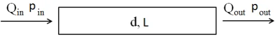
The Dimensionless Dissipative NumberDn is used as a reference parameter to compare different
frequency responses. To evaluate the effect of this dissipative constant an m-file code was prepared. This code shows the Magnitude and phase plots of outlet pressure respect to normalized frequency as shown in Figure2. This figures is based on the following fluid (oil) properties: ρ = 870kg/m3,
17.5∗10−6m2/s<µ<875∗10−6m2/s; 0.01< Dn <0.5 ;βe =1.07∗107Pa; pipe length ofL=2m
Figure 2.Effect of the Dissipative number into pressure wave magnitude
(function of fluid density and compressibility of the system). LargeDnvalues dump the magnitude
of pressure wave.
Laplace transform of the partial derivative expressions7 and 8 could be rewritten in several matrix forms depending on the inputs and outputs selected. Usingx=0 as pipeline inlet andx= L as the outlet, the matrix form for a pressure input and a flow output is as follows:
" Qi
Qo
#
=
" coshΓx
ZcsinhΓx −
1
ZcsinhΓx
1
ZcsinhΓx
coshΓx −ZcsinhΓx
# " Pi
Po
#
=
"
C11 −C21 C21 −C11
# " Pi
Po
#
(19)
Equation19represent 2 equations and four variables. Knowing flows, solvingpo
po(s¯) =H(s¯)p1(s¯) (20) Matko [17] introduced a simplification for the one-dimensional case yields. Introducing the mass flow rate ˙m, the Continuity equation could be written as: A(Pipe Section)c(Sound Speed)
A c2
∂p ∂t =−
∂m˙
∂x (21)
The Momentum equation (neglecting the effect of gravity) is as follows:
1 A
∂m˙ ∂t +
λ(m˙)
2dA2ρm˙
2=−∂p
∂x (22)
whereλ(m˙)is the pipe friction coefficient as a function of the mass flow rate. Both equations21and 22are linearized and the corresponding PDE system is:
L∂m˙
∂t +Rm˙ =− ∂p
∂x (23)
C∂p
∂t =− ∂q˙
Figure 3.Frequency response magnitude and phase plot for the system shown on1.
whereL=1/Ais the system inductance,R=λ(m˙)m˙/A2ρdis the Fluid Resistance andC=A/c2is
the System Capacitance. The analytical solution of a pipeline system model is obtained by derivation of this linear equations. Using this linearized solution, the equivalent matrix of eq.19is:
" Qi
Qo
#
=
coth(n l)
Zk −
1
Zksinh(n l)
1
Zksinh(n l) −
coth(n l) Zksinh(n l)
"
Pi
Po
#
=
"
K11 −K21 K21 −K11
# " Pi
Po
#
(25)
wheren=p(Ls+R)Cs,lis the length of pipe, andZk=
p
(Ls+R)/Cs.
This simplification introduced by Matko has been tested and the results are similar to the results obtained using the equations 19. Using these linearized equations do not result in computational resources savings, thus Equation19was used to solve the model.
For a fluid withρ = 870kg/m3 , µ = 46∗10−6m2/s, βe = 1.07∗107Pa, L = 2mand inner
pipe diameter ofd = 0.01m, the solution of this dissipative model leads to the frequency response magnitude and phase plots shown in Figure3.
Using invfreqs MATLABR function we obtain the folowing transfer function:
H(s¯) = 30.1¯s
11−2.8e4¯s10+···−1.8e27¯s2+1.7e29¯s+2e32 ¯
s12+247.1¯s11+···+2.3e028¯s2+5.8e29¯s+2e32 (26) 3. Modeling a single Pipeline with leak
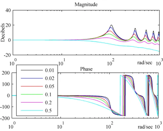
A pipeline with a leak can be modeled as two leak free pipelines connected in series as shown in Figure4. The leak is modeled in the two pipelines joint as an atmospheric flow sink, considering its flux as directly proportional to the pressure gradient and inversely proportional to leak resistance.Rl
is a linear approximation for leak flow resistance,∂p/∂Q. Higher resistances correspond to smaller
leaks. Also, mass conservation equation must be fulfilled at the leak joint:
QlRl =P2a−Patm (27)
Figure 4.Single line with leak
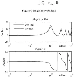
Figure 5.Frequency response plot of a simple line with leak as shown on figure4compared with the same line without leak
From equation19for each line on this scheme we obtain: (Note:The variableXijmeans the value
of propertyXin the pipeline endiof the linej) : Line a:
Q1a=C1aP1a−C2aP2a (29)
Q2a=C2aP1a−C1aP2a (30)
Line b:
Q1b=C1bP1b−C2bP2b (31)
Q2b=C2bP1b−C1bP2b (32)
Equations at leak:
QlRl =P2a−Patm (33)
Q2a=Q1b+Ql (34)
P2a =P1b (35)
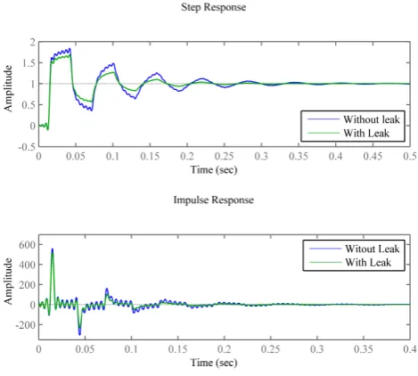
Figure 6.Step and impulse response of the system with and without leak
Obtaining the corresponding rational polynomial transfer functions representing a linear ordinary differential equations of a simple line with and without leak, we could excite the models by a step or impulse signal. Obtained results are shown in Figure6.
4. Oil Brake System
In this section a theoretical, approximated model for a n oil brake system is developed based on previously published results by Wongputorn et al. [18]. In this article, a time domain simulation for hydraulic transients of a brake system is presented for an oil at two different temperatures. Results presented show that in certain circumstances the brake response is slow due to the temperature and suggests an appropriate pipe diameter to overcome this problem. We are going to use the same brake system to simulate the effect of a leak.
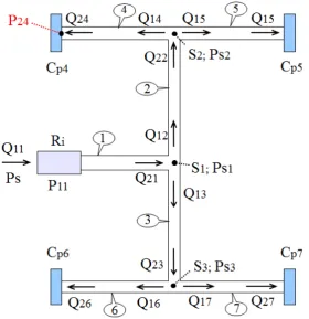
The scheme of the break system without leak is shown in the Figure7
The oil brake system is composed by a pipe system, a brake mechanism (that actuate when receives a pressure increment) and a pedal pump. The pipe system is the group of pipes that connect the pedal to the four brake mechanisms (one for each wheel). The break mechanism is modeled as a tank able to accumulate oil. The pedal is represented as a small tank with a mechanism to get small oil flowQ11and increase the pressure (as a pressure wave)Pswhen braking.
4.1. Fluid properties. Pipeline characteristics.
Oil properties used for simulations are as follows: Densityρ = 880kg/m3; cinematic viscosity ν=300·10−6m2/s; Bulk modulusβ=1, 7235·108Pa.
The pipeline properties are: Pipe diameter d = 0.00635m; line lengths: La = 0.559m;Lb =
0.762m;Lc = 0.7112m;Ld = 2.134m; Bulk modulus of line: Considered incompressible; Brake
mechanisms VolumeV=2, 46cm3
4.2. Theoretical Model and Approximated Model.
Figure 7.Brake System scheme.
Line 1:
Q11Rl =Ps−P11 (36)
Q11=C11P11−C21Ps1 (37)
Q21=C21P11−C11Ps1 (38)
Line 2:
Q12 =C12Ps1−C22Ps2 (39)
Q22 =C22Ps1−C12Ps2 (40)
Line 3:
Q13 =C13Ps1−C23Ps3 (41)
Q23 =C23Ps1−C13Ps3 (42)
Line 4:
Q14=C14Ps2−C24P24 (43)
Q24=C24Ps2−C14P24 (44)
Line 5:
Q15=C15Ps2−C25P25 (46)
Q25=C25Ps2−C15P25 (47)
Q25=C5P25s (48)
Line 6:
Q16=C16Ps3−C26P26 (49)
Q26=C26Ps3−C16P26 (50)
Q26=C6P26s (51)
Line 7:
Q17=C17Ps3−C27P27 (52)
Q27=C27Ps3−C17P27 (53)
Q27=C7P27s (54)
Mass conservation in nodes s1, s2, s3:
Q21=Q12+Q13 (55)
Q22=Q14+Q15 (56)
Q23=Q16+Q17 (57)
The equation system could be also written in the matrix form:
Ps 0 0 0 0 0 0 0 0 0 0 0 0 0 0 0 0 0 0 0 0 0 =
Rt 0 0 0 0 0 0 0 0 0 0 0 0 0 1 0 0 0 0 0 0 0
1 0 0 0 0 0 0 0 0 0 0 0 0 0 C11 −C21 0 0 0 0 0 0 0 1 0 0 0 0 0 0 0 0 0 0 0 0 C21 −C11 0 0 0 0 0 0 0 0 1 0 0 0 0 0 0 0 0 0 0 0 0 C12 −C22 0 0 0 0 0 0 0 0 1 0 0 0 0 0 0 0 0 0 0 0 C22 −C12 0 0 0 0 0 0 0 0 0 1 0 0 0 0 0 0 0 0 0 0 0 C12 −C22 0 0 0 0 0 0 0 0 0 1 0 0 0 0 0 0 0 0 0 0 C22 −C12 −C24 0 0 0 0 0 0 0 0 0 1 0 0 0 0 0 0 0 0 0 0 C14 −C14 0 0 0 0 0 0 0 0 0 0 1 0 0 0 0 0 0 0 0 0 C24 C15 −C25 0 0 0 0 0 0 0 0 0 0 1 0 0 0 0 0 0 0 0 0 C25 −C15 0 0 0 0 0 0 0 0 0 0 0 1 0 0 0 0 0 0 0 0 0 C16 −C26 0 0 0 0 0 0 0 0 0 0 0 1 0 0 0 0 0 0 0 0 C26 −C16 0 0 0 0 0 0 0 0 0 0 0 0 1 0 0 0 0 0 0 0 0 C17 −C27 0 0 0 0 0 0 0 0 0 0 0 0 1 0 0 0 0 0 0 0 C27 −C17
0 0 0 0 0 0 0 0 0 0 0 0 0 1 0 0 0 0 −C4s 0 0 0 0 0 0 0 0 0 0 1 0 0 0 0 0 0 0 0 0 0 0 −C5s 0 0 0 0 0 0 0 0 0 0 0 1 0 0 0 0 0 0 0 0 0 0 −C6s 0 0 0 0 0 0 0 0 0 0 0 0 1 0 0 0 0 0 0 0 0 0 −C7s
0 0 0 0 0 0 0 0 0 0 0 0 0 1 0 0 0 0 0 0 0 0 0 1 −1 0 −1 0 0 0 0 0 0 0 0 0 0 0 0 0 0 0 0 0 0 0 0 1 0 0 −1 0 −1 0 0 0 0 0 0 0 0 0 0 0 0 0 0 0 0 0 0 1 0 0 0 0 −1 0 −1 0 0 0 0 0 0 0 0 0
Q11 Q21 Q12 Q22 Q13 Q23 Q14 Q24 Q15 Q25 Q16 Q26 Q17 Q27 P11 Ps1 Ps2 Ps3 P24 P25 P26 P27
A solution for the pressure of the brake mechanism P24 could be found solving this equation system with the inputPs. The solution was reached using Matlab’sR solve function as is shown in
the m-file appendixA. This solution could be represented as its frequency response magnitude and phase plots. On figure8the frequency response of the analytical model (blue) and the approximated model according the Transfer Function (58) (in red) are represented. Also, in time domain, we could represent the excitation of the approximated transfer function with a step and impulse signals (Fig. 9).
The transfer functionP24(s¯)/PS(s¯) = H(s¯) with the approximated frequency response as the
analytical model is:
H(s¯) = 0.75s
8−801.9s7+····+1.26e17s2+9.46e19s+1.93e21
Figure 8.Frequency response of the theoretical model (blue) and the approximated model (red)
Figure 9.Step and impulse response of the approximated transfer functionP26
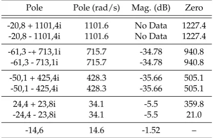
Transfer function pole’s and Zero’s are shown in the table1.
Table 1.Poles and Zeros of the brake system TF without leak
Pole Pole (rad/s) Mag. (dB) Zero
-20,8 + 1101,4i 1101.6 No Data 1227.4
-20,8 - 1101,4i 1101.6 No Data 1227.4
-61,3 -+ 713,1i 715.7 -34.78 940.8
-61,3 - 713,1i 715.7 -34.78 940.8
-50,1 + 425,4i 428.3 -35.66 505.1
-50,1 - 425,4i 428.3 -35.66 505.1
24,4 + 23,8i 34.1 -5.5 359.8
-24,4 - 23,8i 34.1 -5.5 21.0
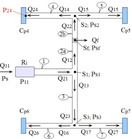
Figure 10.Brake system scheme with leak.
5. Oil Brake System with leak
In this section a model for the previous brake system including a leak is presented. The leak is placed in pipeline 2 as is shown in Figure10. Pipeline is divided at leak point in 2 sub-pipelines, pipeline 2a and pipeline 2b. Two additional equations must be included, mass conservation equation at leak and leak flow equation:
Line 2 is split in Line 2a and line 2b:
Q12a=C12aPs1−C22aPf (59)
Q22a=C22aPs1−C12aPf (60)
Q12b=C12bPf −C22bPs2 (61) Q22b=C22bPf −C12bPs2 (62) Mass conservation at leak and leak flow equations are as follows:
Q22a=Qf +Q12b (63)
RfQf =Pf−Patm (64)
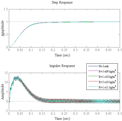
Figure 11.Bode of different leak resistances
Table 2.Absolute values of Poles of TF per Leak value
Rf=5e9 Rf=1e10 Rf=5e10 Rf=1e11
Freq. Freq. Freq. Freq.
(rad/s) (rad/s) (rad/s) (rad/s)
1024.2 1080.6 968.6 930.6
1024.2 1080.6 968.6 930.6
753.6 728.5 715.7 714.8
753.6 728.5 715.7 714.8
432.2 427.9 426.4 426.3
432.2 427.9 426.4 426.3
33.2 34.9 33.26 33.29
33.2 34.9 33.26 33.29
19.3 16.7 12.90 12.98
Table 3.Magnitude of Poles of TF per Leak value
Rf=5e9 Rf=1e10 Rf=5e10 Rf=1e11
Mag Mag Mag Mag
(dB) (dB) (dB) (dB)
No data No data -45.39 -44.6
-41.54 -38.81 -35.75 -35.29
-38.55 -36.94 -35.74 -35.60
-5.62 -5.97 -5.28 -5.26
-2.71 -2.12 -1.30 -1.27
Looking at Figures11and12it can be observed that the leak affects at the frequency response of the system but do not affect the time response velocity of the brake itself. Keep in mind that we are analyzing transients, and then, we are including the effect of loosing oil after some time. Then we will realize that there is a leak in a brake system when we lose some amount of fluid. If a large leak is simulated, the results show that the brake pressure do not reach the expected value, but time response is similar.
Magnitude and position of the transfer function poles obtained for the simulated cases are summarized in Table2. Larger leaks result in lower pole magnitudes located at higher frequencies. By looking at the transfer function obtained using the proposed method we were able to determine the presence of a leak on the pipe system.
6. Conclusions
The governing equations for a fluid transmission system are very complex and do not present an analytical solution that allows to represent its behavior in the time domain. Based on the frequency response of the system, we could obtain an approximated model with equal frequency response and obtain its transfer function. The approximated transfer function model allows to analyze the time domain response, and if needed, compared it with the response of a real model. This comparison, between the approximated model and the real model, could allow us to detect, via software, the presence of leaks.
Vis=300e-6; Den=880; % ISO 46 Oil at 50 F degree
r=0.00635; % r = Internal radius of the line, m values 0.0032 and 0.00635 Be=1.7235e8; % Bulk modulus
c=sqrt(Be/Den); % c = Speed of sound, m/s
Zo=Den*c/(pi*r^2); % Zo = Characteristic impedance constant, r c/pr2 V=2.46e-6; % V = Tank volume, m3
A=0.0111; % A = Brake cylinder piston area, m2
K=3.78e6; % K = Brake cylinder piston return spring constant, N/m La=.559; % L = Line length, m
Dna=Vis*La/(c*r^2); % Dn = Dimensionless dissipative number, nL/cr2 Ld=2.134; % L = Line length, m
Dnd=Vis*Ld/(c*r^2); %Dn = Dimensionless dissipative number, nL/cr2 Lb=0.762; % L = Line length, m
Dnb=Vis*Lb/(c*r^2); %Dn = Dimensionless dissipative number, nL/cr2 Lc=0.7112; % L = Line length, m
Dnc=Vis*Lc/(c*r^2); % Dn = Dimensionless dissipative number, nL/cr2 %
syms s
B=2*besselj(1,j*sqrt(r^2*s/Vis))/(j*sqrt(r^2*s/Vis)*besselj(0,j*sqrt(r^2*s/Vis))); Z=Zo/sqrt(1-B); Ga=Dna*r^2*s/Vis/sqrt(1-B);
Gd=Dnd*r^2*s/Vis/sqrt(1-B); Gc=Dnc*r^2*s/Vis/sqrt(1-B); Gb=Dnb*r^2*s/Vis/sqrt(1-B); % Without Leak
Sol=solve(’Q2=C2a*1-C1a*P2’,’Q3=C1b*P2-C2b*P3’,’Q4=C2b*P2-C1b*P3’,...
’Q5=C1c*P3-C2c*P4’,’Q6=C2c*P3-C1c*P4’,’Q7=C1d*P2-C2d*P5’,... ’Q8=C2d*P2-C1d*P5’,’Q9=C1c*P5-C2c*P6’,’Q10=C2c*P5-C1c*P6’,...
’Q2=Q3+Q7’,’Q4=2*Q5’,’Q8=2*Q9’,’Q6=Cb*s*P4’,’Q10=Cb*s*P6’,... ’P2,P3,P4,P5,P6,Q2,Q3,Q4,Q5,Q6,Q7,Q8,Q9,Q10’);
H=Sol.P4; %
collect(H,s);
H=subs(H,’C1a’,cosh(Ga)/(Z*sinh(Ga))); disp(’Substitute 1’); H=subs(H,’C2a’,1/(Z* sinh(Ga)));disp(’Substitute 2’);
H=subs(H,’C1d’,cosh(Gd)/(Z*sinh(Gd)));disp(’Substitute 3’); H=subs(H,’C2d’,1/(Z* sinh(Gd)));disp(’Substitute 4’); H=subs(H,’C1c’,cosh(Gc)/(Z*sinh(Gc)));disp(’Substitute 5’); H=subs(H,’C2c’,1/(Z* sinh(Gc)));disp(’Substitute 6’);
H=subs(H,’C1b’,cosh(Gb)/(Z*sinh(Gb)));disp(’Substitute 7’); H=subs(H,’C2b’,1/(Z*sinh(Gb)));disp(’Substitute 8’);
N=length(w); wc=[1:1000]; NC=length(wc);
% Bode and phase graph ************************** TFfreqs=subs(H,’s’,j*wc); TFmag=20*log10(abs(TFfreqs)); TFphase=angle(TFfreqs)*180/pi;
g alb = figure(’Name’,’Magnitude and Phase Plot without leak’);
subplot(211);semilogx(wc,TFmag,’b’),title (’P24 Magnitude plot’),ylabel(’Decibels’); subplot(212);semilogx(wc,TFphase,’b’),title (’P24 Phase plot’),ylabel(’Degrees’); % Approximated TF of Model and representation
TFfreqswa=subs(H,’s’,j*w);
[Num,Den]=invfreqs(TFfreqswa,w,7,9,[],100); % Note Release R2008a TFA=tf(Num,Den);
% Approximated TF of model Gain=dcgain(TFA);
TFA=TFA/Gain; Pols=pole(TFA) w0=abs(Pols) Zero=abs(zero(TFA))
TFAfreqs=freqs(Num,Den,w)/Gain; TFAmag=20*log10(abs(TFAfreqs)); TFAphase=angle(TFAfreqs)*180/pi;
g2 alb = figure(’Name’,’Magnitude and Phase Plot withoutleak ’);
subplot(211);semilogx(wc,TFmag,’b’,w,TFAmag,’r’),title(’P24 Magnitude plot’), ylabel(’Decibels’); subplot(212);semilogx(wc,TFphase,’b’,w,TFAphase,’r’),title(’P24 Phase plot’), ylabel(’Degrees’); %
g3 alb = figure(’Name’,’Step and Impulse response without leak’); subplot (211);step(TFA,.5)
subplot (212);impulse(TFA,.5)
References
1. Pal-Stefan Murvay, Ioan Silea, 2012. A survey on gas leak detection and localization techniques. Journal of Loss Prevention in the Process Industries, 966-973.
2. Furness, RA and Reet, JD, 2009. Pipeline leak detection techniques. Pipeline Rules of Thumb Handbook. Elsevier.
3. Kim, Min-Soo and Lee, Sang-Kwon, 2009. Detection of leak acoustic signal in buried gas pipe based on the time-frequency analysis. Journal of Loss Prevention in the Process Industries, 990-994.
4. Lowry, W. E., Dunn, S. D., Walsh, R., Merewether, D., and Rao, D. V. (2000). Method and system to locate leaks in subsurface containment structures using tracer gases. U.S. Patent No. 6,035,701. Washington, DC: U.S. Patent and Trademark Office.
5. Sandberg, C., Holmes, J., McCoy, K., and Koppitsch, 1989. The application of a continuous leak detection system to pipelines and associated equipment. IEEE Transactions on Industry applications, 25(5), 906-909. 6. Tapanes, E. 2001. Fibre optic sensing solutions for real-time pipeline integrity monitoring. In Australian
Pipeline Industry Association National Convention, Vol. 3, pp. 27-30.
7. Weil, G. J., 1993. Non contact, remote sensing of buried water pipeline leaks using infrared thermography. In Water Management in the’90s: A Time for Innovation (pp. 404-407). ASCE.
12. Zhang, J., and Di Mauro, E. (1998). In Implementing a reliable leak detection system on a crude oil pipeline. Dubai, UAE: Advances in Pipeline Technology.
13. USDT, 2007. Leak Detection Technology Study For PIPES Act. Tech. rep., US Department of Transportation. 14. Goodson, R. E. Leonard, R. G., June 1972. A survey of modeling techniques for fluid line transients. Journal
of Fluids Engineering 94, 474–482.
15. Nursilo, W. S., 2000. Fluid transmission line dinamics. Ph.D. thesis, The University of Texas at Arlington. 16. KING, J. D., 2006. Frequency response approximation methods of the dissipative model of fluid
transmission lines. Master’s thesis, The University of Texas at Arlington.
17. Matko, D. e. al., 2000. Pipeline simulation techniques. Math. Comput. Simul. 52(3-4), 211–230.
18. Wongputorn, P., Hullender, D., Woods, R., King, J., 2005. Application of matlab functions for time domain simulation of systems with lines with fluid transients. Journal of Fluids Engineering 125, 177–183.