Simulation of muscle-powered jumping with hardware-in-the-loop
ground interaction
Enrico A. Eberhard
1and Christopher T. Richards
2Abstract— We developed a novel reverse hapticinterface to augment forward dynamic simulations with real-world contact forces. In contrast with traditional haptics, in which a real-world user drives an interaction with a simulated environment, reverse haptics allows a simulated mechanism to probe the real-world environment through a force-sensing robotic manipulator. This method can implicitly extend computer models of biome-chanics and robotic control with complex ground interactions. A 3-DoF manipulator and a biologically inspired musculoskeletal model were developed to test jumping performance on a diverse range of real-world substrates. Jumps were of similar height despite differences in material properties and no active muscle control. Muscle power was lower at the hip, yet total muscle work was higher, against compliant surfaces compared to stiff surfaces. Through reverse haptics, the forces of actuation, inertia and contacts could be measured simultaneously to reveal how intrinsic muscle properties may compensate for substrate dynamics.
I. INTRODUCTION
In biomechanics and mobile robotics, dynamic interactions with the ground are often key to generating motion; it is a by-product of the interactions between actuation forces from muscles or motors (FA), transmission and inertial forces
of the body and limb (FI), and contact forces with the
environment (FC). A change in any of these three elements
will necessarily influence the output of the whole system. For instance, if a soft surface initially provides a lower ground reaction force (GRF) than a hard surface, the net force on the limb and the resultant accelerations will differ.
Unlike electric motors, which have a linear force-velocity relationship, muscle force and power is attenuated strongly and non-linearly by contractile velocity [1]. Consequently, a higher limb acceleration will reduce muscle power capacity more rapidly than a motor. This presents a unique challenge for understanding biomechanics and for building bio-inspired devices in the context of high-power behaviors such as jumping: given the dependence of limb accelerations on GRF, and given the sensitivity of muscle power to limb velocity, how does the natural response of a muscle-like actuator change with substrate?
Substrate-muscle dynamics are challenging to address with experimental biology alone. In vivomeasurements can provide joint torques [2] and muscle power [3], but the con-tributions of individual muscles to accelerating a limb versus the entire body mass is not easily resolved. Additionally, it
This work is funded under FP7-IDEAS-ERC by the European Research Council as part of an ERC-SG-LS4 project (Name: PIPA, ID: 338271)
1PhD Student and2Research Fellow/Supervisor in Paleorobotics at the
Royal Veterinary College (University of London), Hatfield, Hertfordshire, AL9 7TA, [email protected]
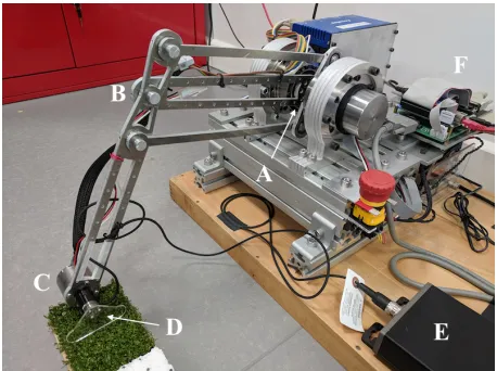
Fig. 1: The 3-DoF robotic manipulator with a tool-side force and torque transducer testing the dynamic response of a substrate. A,B,C: shoulder, elbow and wrist joints, respec-tively. D: the 6-axis transducer (silver) with a foot attachment against artificial turf. E: transducer voltage amplifier. F: DE0-Nano-SoC control board.
is not always possible to determine the center of pressure (COP), the origin of the net GRF vector, especially for multiple contacts or on substrates that transfer forces in a complex way, such as granular media [4].
Fortunately, the above challenges can be approached through simulation or physical models. Multi-body simu-lations of physics have been widely used in both robotics [5] and biomechanics [6] to focus on FA and FI, with
simplified assumptions aboutFC. Advancements in soft
con-tact algorithms also allow the inclusion of collisions and contact forces [7]. While the realistic simulation of complex interactions involving asperity or deformation is possible, it requires considerable parametrization and computation.
An alternative to simulation is physical modelling such as fully biomimetic robots [8], though there is high cost and effort to realistically emulate natural actuation or structure. The resulting robot is also often specialized for one domain; a small shift in research aims, such as scale, may necessitate a redesign. Inspired by recent ”musculo-robotic” approaches [9], we endeavor to solve the above issues by physically modelling the portion of interest (FC) with the remaining
A. Reverse Haptics
Here, we introduce a hybrid simulation-robotic system which we refer to asreverse haptics (RH), combining the favorable elements of simulation and physical modelling. In traditional haptics with impedance control, a user in the real world moves in a virtual environment and receives force feedback [10]. In reverse, the simulation in the vir-tual world probes the real-world environment through a force-sensing manipulator. Hence, the driver and direction of feedback is reversed; from the real-world perspective, instead of displacement-out, force-in, it becomes force-out, displacement-in. While some haptic interfaces exist that use admittance control [10], where the feedback is similarly reversed, the intention is still for a real-world user to drive the interaction.
The RH system comprises two elements: a force-sensing robotic manipulator (Section II) and a simulated muscu-loskeletal model (Section III). The force from the real word is applied to the simulated model, and the resultant displace-ment commands the robot. To demonstrate the technique, a virtual muscle-powered rabbit model was made to jump on various real substrates. The manipulator was also used to measure the intrinsic force-depth response of the materials. Jump performance was explained in terms of interactions be-tween muscle force-velocity properties and substrate contact dynamics.
II. ROBOTIC MANIPULATOR
A. Design
The manipulator is a three degree of freedom (DoF) planar arm with revolute joints (Fig. 1). Arm segments were laser-cut from 6mm aluminum and jointed with ball bearings. The shoulder and elbow joints are each actuated by an EC-60 brushless electric motor (412825, Maxon Motor AG) in line with a 30:1 strain-wave gear (HFUC-20UH-30, Harmonic Drive AG) mounted at the base of the arm. Torque is transmitted to the elbow through a parallelogram linkage. The wrist joint uses a smaller ECi-40 motor (496653, Maxon
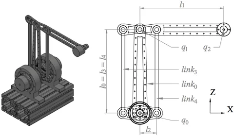
Fig. 2: Render and 2D schematic of manipulator. In this configuration, q0=q1=0, and link1 and link2 are those with lengthsl1 andl2, respectively.
TABLE I: Link parameters
Link l (mm) cx(mm) cz (mm) m(g) Iyy(kgcm2) 0 250 0 73.7 195.8 67 1 250 188.8 0 307.5 138
2 50 0 0 114.8 43
3 250 0 125 66.8 16
4 250 0 125 66.8 16
EE - cxee czee mee Iee
Motor AG) with no reduction. Mounted to the wrist motor shaft is a 6-axis force/torque (F/T) transducer (Nano17, ATI), which in turn can have some end-effector (EE) attachment.
Each electric motor is driven by an Accelus ASP-055-18 digital servo amplifier (Copley Controls) and powered by a 48V supply (LCM1500, Artesyn Embedded Technologies). The robot controller is a DE0-nano-SoC development board with Altera Cyclone V SE FPGA and 925MHz dual-core ARM Cortex-A9 Processor (Terasic). Feedback from 4096-count incremental quadrature encoders (EC-60: 421988 and ECi-40: 488782, Maxon Motor AG) is decoded and differen-tiated in the FPGA for position and velocity. The amplified signal voltages from the F/T sensor are digitized by a 12-bit ADC IC (LTC2308, Linear Technologies).
B. Kinematics
Fig. 2 shows a render of the manipulator next to a simplified schematic. The parallelogram linkage is employed to keep the mass of the driving motors fixed at the base, and is symmetrical aroundlink0for additional stiffness. The five linked segments are coupled such that their kinematics can be described entirely by the two state variables q0 and q1, the rotation oflink0andlink1around theyaxis of the world frame respectively. In the configuration shown in Fig. 2,q0=
q1=0, and both are independent (δq0/δq1=δq1/δq0=0). For each segment i, Table I gives length li, distances of
center of mass (CoM) from the local origin in the X and
Z axes cx,cz, mass m and inertia Iyy around Y at the local
origin. Values for the EE are aluminum on the attachment. The CoM location of each link in theX Zplane in the world frame with respect toq is given by Table II.
C. Dynamics
To remove the effect of the internal dynamics of the robot manipulator on the control, the joint torqueτis modelled in joint space as
τ=M(q)q¨+G(q) +D(q˙) (1)
TABLE II: Forward kinematics of link mass centers
Link x z yrot
0 −cz0sinq0 cz0cosq0 q0
1 cx1cosq1+l0sinq0 l0cosq0+cx1sinq1 q1
2 0 0 q1
3 l2cosq1−cz3sinq0 cz3cosq0−l2sinq1 q0
4 −l2cosq1−cz4sinq0 cz4cosq0+l2sinq1 q0
Torque is defined by the system mass matrixM(q), joint acceleration ¨q, gravity forceG(q), and damping D(q˙)from startup and running torque of the gears. Centrifugal, Coriolis and other forces are not modelled.
The generalized mass matrix is calculated as
M(q) =
4
∑
i=0
JOT
i(q)MxiJOi(q) (2)
where JOi(q) is the Jacobian and Mxi is the mass and inertia tensor of each segment i around its frame origin.
JOi(q)is calculated as the set of partial derivatives for the kinematics of the link frame origins defined by Table II when
cxi=czi=0. The result of (2) can be expressed in a reduced form for the DoFsx,zandyrot.
M
(
q
) =
I
0+
I
3+
I
4+
m
1l
200
0
0
I
1+
I
2+
l
22(
m
3+
m
4)
0
0
0
0
(3)
The forces from gravity can be projected into joint space using the Jacobians of the CoMs of each segment:
G(q) =
4
∑
i=0
JiT(q)Fgi (4)
Fgi is simply
0 0 gmi 0 0 0
T .
G(q) =
−gsinq0(cz0m0+l0m1+cz3m3+cz4m4) −g(cx1m1cosq1+cz2m2sinq1)
0
(5)
Equations (3) and (5) do not include forces from the EE load. The specific mass mee, inertiaIee, and centre of mass
offsetscxee,czeeof the EE depend on the attachment required for a given application. Once these values are known, the following matrices can be added to the existing M(q) and
G(q), respectively:
Mee(q) =
meel20 l0l1meesin(q0−q1) 0
l0l1meesin(q0−q1) Iee+l12mee Iee
0 Iee Iee
(6)
Gee(q) =
−gl0meesinq0
−gmee(cxeecos(q1+q2) +czeesin(q1+q2) +l1cosq1) −gmee(cxeecos(q1+q2) +czeesin(q1+q2))
(7)
Lastly,D(q˙)is interpolated from datasheet values of input torques at various no-load speeds for the HFUC-20UH gears for the shoulder and elbow motors only. Torque is negative w.r.t. velocity and is constrained such that 0≤ |D(q˙)| ≤ |M(q)q¨+G(q)|.
A PD controller is used to command ¨q to track a target state (position and velocity). Torque from (1) is scaled by the gear ratio for the shoulder and wrist motors.
D. Force Sensing
The digitized voltages from the F/T sensor are converted to Cartesian force and torque using an offset and correlation matrix. The offset is temperature dependent and is recalcu-lated before each trial to give zero output in the zero position. Force is sampled at 10kHz and fed through a 4thorder Bessel filter with corner frequency 2.5kHz, chosen for relatively low overhead and phase lag.
III. MUSCULOSKELETAL SIMULATION
MuJoCo 1.50 [11] on a simulation PC (4.0GHz quad-core Intel Core i7-4790K) is used to calculate forward dynamics for a given multi-body model from internal forces (actuation, inertia, gravity and other constraints) and the real external force applied at a designated interface point. The F/T signal is received, and the state of the interface point returned, through raw packet dataframes over 1Gbps Ethernet.
The model in simulation can be designed independently from the manipulator (within the reachable space) to suit the application. Here we describe a biologically inspired model to study muscle-powered jumping.
A. Muscle-Powered Jumper
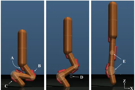
The jumping model is a planar abstraction of a small rabbit (Fig. 3). The model has 4 DoFs: a rotational joint at the hip, knee and ankle, and a sliding joint for the body along the vertical axis. Constraining the body this way mimics two symmetrical legs with cancelling lateral forces as in [12] and reduces complexity.
Each revolute joint is actuated by a single muscle origi-nating on the parent segment, wrapping over a cylinder with radiusr0 and inserting on the child segment.
Fig. 4: Normalized muscle model force fm (blue) and power
pm (red) against relative shortening velocities. Velocity is
positive when shortening, and normalized by muscle resting length (v=δl/δt∗1/l0). Force is normalized by fmax. Max
power pmax is achieved at velocityvpmax=5.13.
B. Muscle Model
The muscle force fm is calculated using a standard
Hill-type contractile element with dependence on velocity, but not length. Force is positive in the shortening direction, and
fm≥0.
fm=a∗fv(v)∗fmax (8)
1) Activation: A first order activation of a control input 0≤u≤1 [6]. Time constants for activation τA and
deacti-vationτD are 0.01 and 0.04 seconds, respectively.
˙
a=u−a
τ (9)
τ=
(
τA(0.5+1.5a) u>a
τD
0.5+1.5a u≤a
(10)
2) Force-velocity relation: The force generating property of the muscle actuator is adapted from [13] and gives the curve in Fig. 4. Velocity is defined as positive when the muscle is shortening; fv(0) =1 and fv(vmax) =0. The
pa-rameterh(Hill constant) determines the slope; fv(v)becomes
linear (towards the idealized electric motor) ash→∞. It is worth nothing that bothpmaxand
Rvmax
0 pv(v)dvare more than
doubled whenh→∞compared to standard muscleh.
fv(v) =
( vmax−v
v/h+vmax v>0
1+ 4v(h+1)
v(h+5)−4hvmax v≤0
(11)
TABLE III: Muscle parameters
Extensor fmax(N) vmax(l0s−1) h l0 (mm) r0(mm)
Hip 80 15 0.37 60 8
Knee 50 15 0.37 60 8
Ankle 75 15 0.37 40 15
C. Model Parameters
All values for body and muscle anatomy are loosely based on data from [14] and [15]. Total simulated body mass is 400g, with a distribution of 65%, 20%, 10% and 5% for the body, upper leg, lower leg and foot respectively. Lengths are 60mm for upper and lower leg, and 40mm for the foot, with capsule segments of radius 10mm. Rabbits have multiple muscles at each joint (5, 2, and 3 at the hip, knee and ankle); for each single representative muscle, l0 and r0 are a rounded and weighted average of the contributing muscle by respective mass, and fmax is summed (Table III). [12]
references vmax=15 for small mammals, and h=0.37 is
from [13]. Joint boundaries were applied at 0◦ to prevent over-extension (Fig. 3, right) and at 135◦ (60◦ for the hip) at the most folded (Fig. 3, left).
IV. INTERFACE TIMINGS
For consistent interactions with the real-world environ-ment, the simulated physics time must be continuous and proportional to real time. The round-trip time (RTT) of each state-out, force-in transmission is measured, and the forward dynamics simulation stepped in the required number of small increments to match the time difference. Any variance in RTT affects neither continuous physics time nor the accuracy of the physics solver.
RTT is limited by the communication rate between the simulation and the robot, not by the forward dynamic simu-lations. The simulation PC achieves a forward dynamics step rate of 250kHz for a swinging double pendulum benchmark example, allowing a minimum timestep of 4µs to keep up with real-world time. The communication rate between the robot and PC is currently 1kHz. By optimizing IRQ handling on the Linux kernel and migrating control and communication routines to the FPGA, future RTT < 50µs (20kHz) is possible [16].
RTT should be low when EE accelerations are high to reduce the displacement in simulation before force feedback. If time-dependence is not important (i.e. force-velocity prop-erties of substrates is ignored), RTT can be lowered virtually by evaluating the simulation at a proportionally slowed time factor; the following experiments were performed 20 times slower than real-time to simulate the higher future communication rate, and the results are still valid in the context of substrate force-depth properties.
V. JUMPING EXPERIMENTS
A. Surface Materials
A set of materials was chosen to test the reverse haptic simulator (Fig. 5). Each exhibits a different force-depth
erty (Fig. 6). Rubber has a stiff response with a sharp but lin-ear increase. Cardboard is initially compressible but quickly levels out. The foam follows the same initial compression as the cardboard but continues linearly with a slightly higher stiffness than the rubber. The blades of artificial turf have almost no resistance until they are compressed and linearly compliant. Finally, the sponge exhibits the opposite profile; initially linear and highly compliant, it slowly levels out at large depth. Additionally, there is plastic compression in the foam and turf, which stay partly deformed after large forces. On these, subsequent trials were moved laterally by 5mm to a fresh section.
B. Experimental Procedure
To evaluate how a muscle-powered jumper naturally re-sponds to a change in substrate, an EE attachment with the same 40mm length and 10mm radius as the simulated foot was laser-cut from 3mm acrylic. The following conditions were used for the described model on each material. The initial joint angles at the knee and ankle were set to folded limits of 135◦, and the hip angle was set to 36◦so that the tip of the foot was directly under the body. The starting height of the jumper was adjusted for each material so that the tip of the foot was barely in contact with the surface (the first point at which any GRF was measurable). The control signal
u and activation a of all muscles was initially 0, before a step change ofu=1 att=0.05 seconds. The interface with the robot was terminated after 0.2 seconds to avoid landing forces, and the CoM height trajectory projected forward from passive dynamics. Data from five trials on each material were resampled to a common duration and interval using linear interpolation before averaging results by surface.
VI. RESULTS
The muscle-powered jumper effectively interacted with the various substrates through the reverse haptic interface to achieve jumps of similar height, despite no change in muscle
Fig. 6: GRF from materials with increasing depth at low velocity penetration. Trials were started above each surface with the flat edge of a foot attachment (see section V-B) moving downwards at 0.5mms-1. Depth 0 is where force first exceeds 0.1N.
Fig. 7: The mean CoM on the Z axis of the muscle-jumper (Fig. 3) on each surface (Fig. 5) throughout the jump. CoM data is shifted to be 0 at t =0. Muscles are activated at
t=0.05 (dotted).
activation. The following error between the target state in simulation and the state of the manipulator was within 0.2mm (including latency-induced error). Peak GRF forces ranged 18-27N across surfaces (5-8 times body weight) which is realistic for an animal of that scale [12].
Across all surfaces, there is a similar initial drop in CoM height from limb compression before muscle activation (Fig. 7). Post activation, in softer materials (turf, sponge) the CoM drops further as the limb extends downwards, while in firmer materials the CoM starts to lift almost immediately. The highest jump was on sponge (most compliant), while the lowest was on rubber (least compliant).
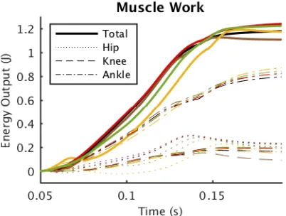
The main difference in muscle performance between sur-faces is at the hip (Fig. 8). Apart from a rightwards shift in timing, hip work is lower in softer surfaces. On turf and sponge, potential energy is initially converted to kinetic energy as the limb sinks into the substrate (Fig. 9). After
Fig. 8: Cumulative muscle work output over time for each surface, calculated as the integral of muscle power, where
pm=fmvm. For each surface (colors as in Fig. 7), the work of
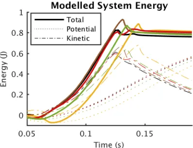
Fig. 9: Mean energy of the musculoskeletal model for each surface (colors as in Fig. 7). The kinetic (dashed) and poten-tial (dot-dash) energies of the rigid bodies were calculated and summed (solid) at each time-step in MuJoCo. Potential energy is set to 0 att=0.
activation, negative hip power reduces kinetic energy, even as the knee and ankle extensors work to increase it. Perhaps as a result of the hip slowing limb extension (hence increasing contact duration), total muscle work at time of take-off is highest in the softer materials.
Fig. 10 illustrates how external dynamics can be implicitly reconstructed using RH. By subtracting muscle energy con-tribution (Fig. 8) from energy in the simulated system (Fig. 9), the absorption and return of energy in the substrate can be estimated. The stiffer surfaces (rubber, cardboard) return absorbed energy rapidly, and the peak-to-peak difference is small. Foam also returns some energy, but more slowly and to a lesser magnitude. The turf and sponge both absorb more energy directly after activation, but the sponge returns more stored energy to the system than turf, and does so at a low power. Counterintuitively, the slow energy return on sponge may improve jump performance compared to the other surfaces because of the power-limited nature of muscle.
VII. CONCLUSION
Reverse haptics gives unique access to measure and ma-nipulate all elements (FA, FI, FC) of a dynamic system
to build a better understanding of the parameter space. Here we found that muscle may compensate for substrate dynamics without external control, with the hip extensor delaying power in softer substrates to increase total work. In future work, this method will be used to address biological questions of control strategies for specific behaviors and the affect of limb morphology on natural surfaces, including granular and fluid media. Further to bio-inspired research and engineering, reverse haptics may also be a gateway for simulated agents with reinforcement learning to interact with rich and varied environments.
REFERENCES
[1] F. E. Zajac, “Muscle and tendon: Properties, models, scaling, and application to biomechanics and motor control,”Critical Reviews in Biomedical Engineering, vol. 17, no. 4, pp. 359–411, 1989.
Fig. 10: Difference in energy contribution of muscles (Fig. 8) and model energy (Fig. 9) for each surface. Negative slopes represent energy absorption, and positive slope is energy return. The sharp decline before 0.15s is energy loss from joints reaching extension limits and coincides with take-off.
[2] L. B. Porro, A. J. Collings, E. A. Eberhard, K. P. Chadwick, and C. T. Richards, “Inverse dynamic modelling of jumping in the red-legged running frog, Kassina maculata,”The Journal of Experimental Biology, vol. 220, pp. 1882–1893, May 2017.
[3] E. K. Moo, D. R. Peterson, T. R. Leonard, M. Kaya, and W. Herzog, “In vivo muscle force and muscle power during near-maximal frog jumps,”PLOS ONE, vol. 12, no. 3, p. e0173415, 10-Mar-2017. [4] J. Aguilar and D. I. Goldman, “Robophysical study of jumping
dynamics on granular media,”Nature Physics, vol. 12, pp. 278–283, Nov. 2015.
[5] T. Erez, Y. Tassa, and E. Todorov, “Simulation tools for model-based robotics: Comparison of Bullet, Havok, MuJoCo, ODE and PhysX,” pp. 4397–4404, IEEE, May 2015.
[6] M. Millard, T. Uchida, A. Seth, and S. L. Delp, “Flexing Computa-tional Muscle: Modeling and Simulation of Musculotendon Dynam-ics,”Journal of Biomechanical Engineering, vol. 135, pp. 0210051– 02100511, Feb. 2013.
[7] G. Gilardi and I. Sharf, “Literature survey of contact dynamics modelling,”Mechanism and Machine Theory, vol. 37, pp. 1213–1239, Oct. 2002.
[8] A. J. Ijspeert, “Biorobotics: Using robots to emulate and investigate agile locomotion,”Science, vol. 346, pp. 196–203, Oct. 2014. [9] C. T. Richards and C. J. Clemente, “A bio-robotic platform for
integrating internal and external mechanics during muscle-powered swimming,” Bioinspiration & Biomimetics, vol. 7, p. 016010, Mar. 2012.
[10] D. Escobar-Castillejos, J. Noguez, L. Neri, A. Magana, and B. Benes, “A Review of Simulators with Haptic Devices for Medical Training,”
Journal of Medical Systems, vol. 40, Apr. 2016.
[11] E. Todorov, T. Erez, and Y. Tassa, “MuJoCo: A physics engine for model-based control,” inIntelligent Robots and Systems (IROS), 2012 IEEE/RSJ International Conference On, pp. 5026–5033, IEEE, 2012. [12] R. M. Alexander, “Leg Design and Jumping Technique for Humans, other Vertebrates and Insects,”Philosophical Transactions of the Royal Society B: Biological Sciences, vol. 347, pp. 235–248, Feb. 1995. [13] T. J. Roberts, “Probing the limits to muscle-powered accelerations:
Lessons from jumping bullfrogs,”Journal of Experimental Biology, vol. 206, pp. 2567–2580, Aug. 2003.
[14] R. L. Lieber and F. T. Blevins, “Skeletal muscle architecture of the rabbit hindlimb: Functional implications of muscle design,”Journal of morphology, vol. 199, no. 1, pp. 93–101, 1989.
[15] J. A. Rose, Hindlimb Morphology in Eastern Cottontail Rabbits (Sylvilagus Floridanus): Correlation of Muscle Architecture and MHC Isoform Content with Ontogeny. Master of Science, Youngstown State University, May 2014.
[16] W. M. Zabolotny, “Low latency protocol for transmission of measure-ment data from FPGA to Linux computer via 10 Gbps Ethernet link,”