Modeling Mobile Edge Computing Deployments for
Low Latency Multimedia Services
Jorge Mart´ın-P´erez*
†, Luca Cominardi
†, Carlos J. Bernardos
†, Antonio de la Oliva
†, Arturo Azcorra
†‡ †Universidad Carlos III de Madrid, Spain
‡
IMDEA Networks Institute, Spain
Abstract—Multi-access Edge Computing (MEC) technologies bring important improvements in terms of network bandwidth, latency and use of context information, critical for services like multimedia streaming, augmented and virtual reality. In future deployments, operators will need to decide how many MEC Points of Presence (PoPs) are needed and where to deploy them, also considering the number of base stations needed to support the expected traffic. This article presents an application of inhomogeneous Poisson point processes with hard-core repulsion to model feasible MEC infrastructure deployments. With the presented methodology a mobile network operator knows where to locate the MEC PoPs and associated base stations to support a given set of services. We evaluate our model with simulations in realistic scenarios, namely Madrid city center, an industrial area, and a rural area.
Index Terms—5G, MEC, Point Process, Deployment, Charac-terization, Network Slicing, Streaming, Low Latency, Augmented Reality, Virtual Reality.
I. INTRODUCTION
The next generation of mobile networks, the so-called 5G, comes with the promise of new and enhanced services, through the introduction of an improved radio interface, plus a network core that allows to dynamically deploy services closer to the location of the users. 5G networks will need to accommodate on top of the same physical infrastructure multiple kinds of services with very distinct requirements, spanning from ultra-low latency to high bandwidth and high reliability. These services are grouped in three main categories by 3GPP: enhanced Mobile Broadband (eMBB), Ultra-Reliable and Low Latency Communications (URLLC), and Massive Internet of Things (MIoT) [1].
Among the several use cases that may be supported by 5G are Augmented Reality (AR) and Virtual Reality (VR), which can be included into eMBB and URLLC categories. In particular, AR/VR impose a Motion to Photon (MTP) latency that does not exceed 20 ms, requiring a network Round Trip Time (RTT) below 2 ms [2]. Moreover, a response within 1 ms is desired in case of visual-haptic interaction [3]. Al-though the new 5G radio interface promises ultra low latency enhancements, to truly fulfill the VR/AR ultra-low latency requirements it is also necessary to reduce the communication
*Corresponding author: [email protected]
Parts of this paper have been published in the Proceedings of the IEEE BMSB 2018, Valencia, Spain
Work partially funded by the EU H2020 5G-CORAL Project (grant no. 761586) and by the EU H2020 5G-TRANSFORMER Project (grant no. 761536).
Mobile edge host / MEC PoP
Mobile edge platform
Virtualization infrastructure ME
app ME app
ME app
Service Mobile edge
platform manager Mobile edge orchestrator
Virtual infrastructure manager Operations Support System
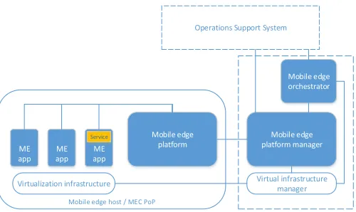
Fig. 1: ETSI MEC architecture.
distance by bringing the multimedia applications close to the end users. This is achieved by Multi-access (Mobile) Edge Computing (MEC) [4] [5].
MEC is a key enabler for 5G technology and its main principle is to host computation and storage at edge hosts, close to end users. Typically, these edge hosts are highly distributed in the network, located close to the radio access network nodes (e.g., gNodeBs in 5G). As a result, MEC en-ables two types of services: (i) low-latency services, requiring a very low and bounded delay between the end user device and the server hosting the application; and, (ii) context-aware services, which need to access end-user contexts, such as the user channel quality conditions, in order to adapt the delivered service. MEC is being standardized within ETSI, via the MEC ISG group. A simplified version of the MEC architecture defined by ETSI is shown in Fig. 1. The main components of the architecture include: the Mobile Edge (ME) host, the ME application and the MEO (ME orchestrator). The MEC host is the key element. It provides the environment to run ME applications, while it interacts with the mobile network entities, via the Mobile Edge Platform (MEP), to provide ME services and deliver mobile traffic to MEC applications.
scenario deployments, analyzing how many MEC Points of Presence (PoP) are needed to meet a given set of requirements. This work has been done within the framework of the 5G-TRANSFORMER project. The 5G-5G-TRANSFORMER main goal is to support vertical industries (particularly focusing on low latency) through flexible slicing and federation of resources across multiple domains. This article is structured as follows: Section II introduces related work, Section III presents in detail our model, which is then applied to a realistic scenario in Section IV and validated in Section V. Finally, Section VI concludes this article with some final remarks and hints for future work.
II. RELATEDWORK
Existing work in the literature, such as [6], studies feasi-ble network infrastructure deployments using Point Processes (PPs) that randomly scatter points on some space (e.g., a line, a Cartesian plane, etc.). In particular [6] uses Poisson PPs (PPPs), a family of PPs used to generate the location of base stations (BSs) that are distributed following Poisson counting processes. PPPs can impose a minimum distance between BSs to increase coverage area and reduce the interference (see hard-core PPPs in [7]), and control if every region in the space has the same or different probability to host a BS (see homogeneous andinhomogeneousPPPs, respectively, in [7]). Different types of PPPs are used in the State of the Art (SoA). For instance, the authors of [8] use Neyman-Scott [9] PPPs to generate small base stations (BSs) clustered around macro BSs with the objective of modeling the coverage and interference in heterogeneous networks. Similarly, [10] shows that homogeneous PPPs can be used in realistic deployment scenarios to reduce interference and increase the coverage area by properly configuring the distance between the BS sites and the intensity parameter.
Works like [6] and [11] analyze potential infrastructure deployments with the help of homogeneous PPPs. The for-mer focuses on studying the cost of a Cloud Radio Access Network (Cloud-RAN) infrastructure using PPPs, while the latter analyzes the throughput and coverage of end users, using PPPs to determine hotspot locations in heterogeneous cellular networks.
Regarding future MEC deployments in real scenarios, [12] studies the existing BS deployment in several USA locations (including highways and rural areas). Likewise, [13] characterizes AR/VR deployments in stadium scenarios in the perspective of forthcoming Tokyo 2020 Olympics. The authors conclude that such use case requires a single media room dedicated to the video processing and proposes two distinct BS deployments: one powerful BS in the stadium (e.g., on the roof) or multiple small BSs (e.g., located close to the stadium vomitoria1).
The work presented in this article studies the deployment of MEC PoPs in real urban, industrial and rural scenarios to satisfy the 5G slices requirements, including the most stringent latency expected by the 5G AR/VR applications (as done in [13]).
1A vomitorium is a passage situated below a tier of seats in a stadium.
Unlike [12], this paper accounts for 5G New Radio (NR) technologies rather than legacy radio technologies. We gener-ate feasible locations for gNodeBs, and derive deployments of MEC PoPs guaranteeing low latency requirements that deploy-ments in [12] do not ensure. We use inhomogeneous Mat´ern II PPs (see Proposition III.2 in Sec. III-A for more details) to obtain feasible locations for the BSs. The inhomogeneity of these processes improves the Mat´ern PPs in the SoA by locat-ing the BSs based on the density of population. That is, more BSs are generated where the population density2 is higher. In other words, the inhomogeneity allows to concentrate the BSs where they are really needed and to minimize the generation in those areas with little traffic demand.
The generated BS locations are used next to derive the required number of PoPs and their potential location.
III. MODEL
This section presents the model used to both generate the BSs of future MEC deployments, and to determine the locations of the MEC PoPs to which the BSs are assigned. In our model a BS is the first connection point in the RAN accessed by the User Equipment (UE), for example a 2G BS, a 3G NodeB, a 4G eNodeB, or a 5G gNodeB. In Sec. III-A we extend Mat´ern PPs to introduce inhomogeneity and generate BSs based on the population density. The derived processes, namely inhomogeneous Mat´ern I and II PPs, impose a minimum distance between BSs to obtain a better coverage. Moreover, we show that Mat´ern II PPs are more suitable for BSs generation because of their relaxed thinning procedure. Sec. III-B presents the algorithm used to generate MEC PoPs that can satisfy imposed latency constraints among all the BSs that are assigned to them.
A. Macro cells generation
With the model we aim to generate more BSs in regions where the population is higher. Here we refer to a region
R as a subset of a complete separable metric space R, for example a map of Spain. Hence R can represent a city like Madrid and the model locates BSs in city areas where there are more people. To achieve this we consider that every region
R contains population circles Ci ⊂R defined by a centerci
and a revolution functionfi(x)(withi∈[1, RC]∩N, andRC
the number of population circles defined inside the regionR). Therevolution functionfi(x)withx∈Cidetermines where
it is more likely to have a person in Ci. This function leads
to a surface of revolution defined atCi that can be expressed
as fi(kx−cikd), and which height expresses the amount of
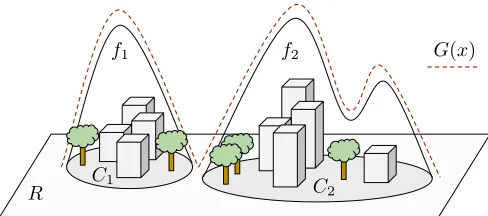
people at a given location x∈R. Therefore, the presence of people atx∈R is expressed as:
G(x) :=X i
fi(kx−cikd), ∀Ci⊂R, ∀d∈N (1)
where G(x) is referred as gentrification in the following paragraphs.
2In our scenarios we refer to human population. Nevertheless,
f1 f2
C1 C
2
G(x)
R
Fig. 2: Revolution functions of a region with two building areas.
Figure 2 illustrates an example of a region R with two population circles (i.e.,C1,C2) corresponding to two distinct
areas. Moreover, therevolution functionsfi considered in this example are Gaussian-like surfaces of revolution that can be multi lobed as the case of f2, and thegentrification function
G(x)is just the dashed line merging both of them.
If an inhomogeneous PPP uses the gentrification function
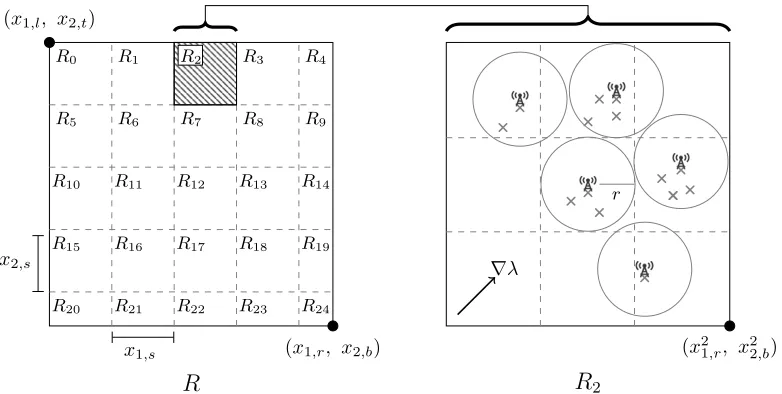
G(x), the process generates BSs in concordance with the population, but it is still necessary to know how many we have to generate. Based on [14] we grid the region R in cells to satisfy the imposed number of BSs per km2 in future 5G deployments, and we take Ras a two dimensional space where the region to be gridded R⊂ R (for example Madrid) is expressed as a rectangle R = [x1,l, x1,r]×[x2,b, x2,t]
divided into cellsRi⊂Rof widthx1,s and heightx2,s. The
resulting grid haswi rows anduicolumns that are completely determined by the cell index i (which increases from left to right, and upside down as shown in Fig. 3):
wi:=
i·x
1,s un
, ui=i·x1,s modun (2) un=
x1,s−x1,l x1,s
(3)
withunbeing the number of columns of the gridded regionR.
Finally, we set each cell Ri as the product of two intervals Ri = [xi1,l, x
i
1,r]×[xi2,b, x i
2,t]whose limits are:
xi1,l=x1,l+x1,sui (4) xi1,r= min{x1,r, x1,l+ (1 +ui)x1,s} (5) xi2,b= max{x2,b, x2,t−(1 +wi)x2,s} (6) xi2,t=x2,t−x2,swi (7)
Fig. 3 illustrates on the left-hand side (lhs) the limiting coordinates of a region R that is gridded into cells Ri
according to the limits above, i.e., (4)-(7).
In every single cell an inhomogeneous PPP generates a specific average number of BSs using an intensity function defined as λ(x) = k·G(x) (where k ∈ N is a constant),
so BSs are located with higher probability where there are more people. But since we want to have the BSs as sparse as possible, it is necessary to impose a minimum distance between them. This work leverages the Mat´ern hard-core processes [15] to model the BSs’ generation. The first process under consideration for our model is the Mat´ern I process.
Definition III.1. Mat´ern I point process: is the point process obtained after applying athinningwith index function:
I1(x, X) :=
(
0 ifN(B(x, r))>1
1 ifN(B(x, r)) = 1 (8)
to astationaryPPPX, whereN(B(x, r))denotes thenumber of points of the point process X falling in the ball centered atxwith radiusr.
In other words, a point x ∈ X is removed if it has a neighborx0 ∈X with distancekx−x0kd < r. This property
suits the random generation of the BSs’ locations because only one BS can be in a neighborhood. However, these point processes arestationary(see [7]), and thereforehomogeneous, before thethinning(see Definition III.1), but this model uses inhomogeneous PPPs to generate BSs (based on G(x)) at each cell Ri ⊂ R. Thus we modify the original definition of a Mat´ern I point process to use an inhomogeneous PPP before the thinning. We call these processes inhomogeneous Mat´ern I PPs.
After inhomogeneity is introduced, we need to know an expression for the average number of points E[N(C)] that
can appear in a certain set C ⊂ R. The reason, as shown in Proposition III.1, is that this expression is in terms of the repulsion radius r and the intensity function λ(x), and we must select these parameters accordingly to generate the desired average number of BSs in a cellRi. Since there is no expression in the literature for the average number of points of a “inhomogeneous Mat´ern I PPs”, we have obtained it with the help of the Campbell-Mecke formula [16].
Proposition III.1. Given an inhomogeneous PPP X with intensity functionλ, and thethinningfunctionI1, the resulting
thinned point process, calledinhomogeneous Mat´ern IPP, has the following averagenumber of pointsatC:
E[N(C)] :=
Z
C e−
R
B(x,r)λ(u)duλ(x)dx (9)
wherer is thethinningradius ofI1.
Proof. First we define the auxiliary functiong:
g: R ×Ω→ {0,1} (10)
(x, A)7→1C(x)1(dist(x, X\x)> r) (11)
whereΩis the space of events (see [7]). We can then rewrite the average number of points atC as:
E[N(C)] :=E
X
x∈X
R0 R1 R2 R3 R4
R5 R6 R7 R8 R9
R10 R11 R12 R13 R14
R15 R16 R17 R18 R19
R20 R21 R22 R23 R24
R2 (x1,l, x2,t)
(x1,r, x2,b) x1,s
x2,s
R
R
2(x2
1,r, x22,b) r
∇λ
Fig. 3: Gridded region on the left side, and macro cell generation inside a cell on the right side. Gray crosses without a cell tower represent BS points that did not survive after the I2 thinning. The rhs shows how the region cell R2 is gridded when
the repulsion radius is chosen as specified in Eq. (25) with N(R2) = 5.
Next, we use the Campbell-Mecke formula to obtain:
E
X
x∈X
g(x, X) :=
Z
R
Ex[g(x, X)]λ(x)dx= (13)
=
Z
R
Z
Ω
g(x, X)Px(A)dA λ(x)dx= (14)
=
Z
C
Z
Ω
1(dist(x, X\x)> r)Px(A)dA λ(x)dx= (15)
=
Z
C
Px(dist(x, X\x)> r) λ(x)dx= (16)
=
Z
C
P(N(B(x, r)) = 0) λ(x)dx (17)
wherePx denotes the Palm probability. Finally, we apply the
capacity functional (see [7]) of a PPP to obtain the stated equality.
One drawback of these “inhomogeneous Mat´ern I” pro-cesses is their very restrictive dependent thinning procedure, which might reach the case where all the points are re-moved in certain neighborhoods. To overcome such limitation, our model considers a second type of processes, known as Mat´ern IIpoint processes, that rely onmarked point processes (see [7]). Mat´ern II processes assign a mark to every point generated so as to allow the dependent thinning processes (see [7]) distinguish which point is retained in a neighborhood.
Definition III.2. Mat´ern II point process: is the point process obtained after applying a thinningwithindex function:
I2(x, m, X, MX) :=
1 if m= minm0∈M
X
(x0, m0) :
x0∈B(x, r)
0 otherwise
(18) to a stationary markedPPP X, where MX denote the marks associated to the point processX.
In other words, among all the points falling in the ball of radiusr, only the one with the lowest markmsurvives. These kind of processes present the advantage that even when the intensity functiontakes high values, at least one point remains in every neighborhood. In our model this means that in a certain neighborhood there is no more than one BS.
If rather than using a stationary PPP before applying the dependent thinning I2, we use an inhomogeneous PPP
(something novel in the SoA); then it is possible that the retained BS in a neighborhood is the one with higherλ(x)by choosing the mark (x, m) as m ∼ 1
λ(x). But still is missing
how we can control that a correct number of BSs is generated at each region Ri ⊂R based on the repulsion radius r and
the intensity function λ(x). Thus we proceed as with the “inhomogeneous Mat´ern I” PPs to obtain an expression for the average number of points(something novel in the SoA).
Proposition III.2. Given aninhomogeneousmarked PPP X withintensity functionλ, thethinningfunctionI2, and marks
m∼ 1
λ(x), the resulting thinned point process, called
inhomo-geneous Mat´ern II PP, has the following average number of pointsatC:
E[N(C)] :=
Z
C e−
R
B(x,r)1(λ(u)>λ(x))λ(u)duλ(x)dx (19) wherer is thethinningradius ofI2.
Proof. As in the proof of Proposition III.1, we proceed defin-ing the functiong:
g: R ×Ω→ {0,1} (20)
(x, A)7→1C(x)1
λ(x) = max
x0∈X∩B(x,r){λ(x
0)}
(21)
formula as in the previous proof and we obtain the average number of points as:
E
X
x∈X
g(x, X) :=
Z
C Px
λ(x) = max x0∈X∩B(x,r)
λ(x)dx=
(22)
=
Z
C
P N B>λ(x)(x, r)
= 0
λ(x)dx= (23)
=
Z
C e−
R
B(x,r)1(λ(u)>λ(x))λ(u)duλ(x)dx (24)
whereB>λ(x)(x, r) ={u:x∈B(x, r)∧λ(u)> λ(x)}.
The right-hand side (rhs) of Fig. 3 depicts how to obtain BSs’ locations using an inhomogeneous Mat´ern IIPP (whose average number of points is derived in Proposition III.2). First, it generates the gray crosses using an inhomogeneous PPP with intensity function λ(x)(note that more points are generated on the upper right corner because of the direction of ∇λ(x)). Then, aI2thinning is applied using repulsion radius
rwith marksm∼ 1
λ(x), so only the gray cross with the most
top-right coordinate falling within a ball of radius r survive. This surviving cross is hence illustrated as a cell tower in Fig. 3.
As both Propositions III.1 and III.2 state, the average number of points of “inhomogeneous Mat´ern I and II” PPs depend on the repulsion radiusr. Then for a cellRi⊂ R, we
need to know which r allows the generation of the required number of BSs. To generate N(Ri) points we set the cell
repulsion radius as:
r:= 2
√
x1,s·x2,s
dp
N(Ri)e (25)
which grids Ri in cells that can contain the repulsion balls
B(x, r) of the Mat´ern PPs. These new cells are squares of side 2rand area 4r2 > πr2=|B(x, r)|, and they divide the parent cell Ri in d
p
N(Ri)e2 smaller cells that can host a
whole macro cell repulsion area.
B. MEC PoPs’ deployment
We assign the traffic of every BS generated in Sec. III-A to a MEC PoP that is deployed somewhere within the operators’ network infrastructure, and at a specific geographic location (i.e., to minimize RTT). The further the distance between the MEC PoP at locationm, and a BS at locationx, the higher the propagation delayl(·)of the link connecting them. The other two contributions for the packet Round Trip Time (RTT) are the radio transmission delay tr between a BS and the final user, and the packet processing delay p(·):
RT T := 2l(kx−mkd) + 2p(M) +tr (26)
with p(M) denoting the processing delay introduced by the network hops to be traversed to reach the network ring M. Hence, our model envisions the operator infrastructure as a hierarchy of network ringsM, in which traffic traverses more hops to reach network rings that are higher in the hierarchy (see Fig. 4). That is, taking ≺ as a relationship expressing which network ring is higher in the network hierarchy M, if
Ma, Mb ∈ M and Ma ≺Mb, we can say that a MEC PoP
deployed atMa is reached in less hops than one atMb. Thus, p(Ma)< p(Mb), and network ring Ma aggregates less traffic
thanMb.
So if we place a MEC PoP at location m and assign it to network ring M, after fixing the maximum RTT and radio technology, from Eq. (26) we know the maximum distance to those BSs whose traffic is assigned to the new MEC PoP
kx−mkd≤l−1
RT T−2p(M)−t
r 2
=mM (27)
Algorithm 1 determines the MEC PoPs’ deployment in three stages:
1) Initialization: the first stage (lines 1-4) creates the set of MEC PoPs locations, the set of their network rings, the set of BSs and one matrix of locationsx∈Rper network ring. Each entry xin the matrix matrices[M] represents the number of BSs that can be assigned to a MEC PoP deployed at a given location xand associated to the ring
M ∈ M
2) Candidates search: this second stage (lines 5-10) deter-mines how many BSs can be assigned to a MEC PoP depending on its location and associated network ring
M ∈ M. For every M it loops through each BS and increases by one those location entries of matrices[M]
satisfying that if a MEC PoP is deployed there, it could satisfy the RTT and hence, the BS could be assigned to that MEC PoP. If matrices[Ma][x0] = 4 after this stage,
it would mean that a MEC PoP associated to Ma and
deployed atx0 would have 4 BSs assigned to itself.
3) MEC PoPs selection: this third and last stage (lines 11-35) is the main loop of Algorithm 1, and each iteration decides a new MEC PoP location and network ring. It comprises two phases:
a) MEC PoP location: this phase (lines 15-24) obtains the best location where a MEC PoP can be located. It iterates through all the possible network rings in M searching for the location where the maximum amount of BSs can be assigned to a MEC PoP. In case of having multiple locations assigning the same amount of BSs at different rings, let’s call themMa, Mb, then the algorithm selects the location related to the ring with the minimum propagation delay, i.e.,min{p(Ma), p(Mb)}.
b) Assignment update: the MEC PoP obtained in the previous step handles the traffic of up to maximum number of BSsringMaxBSs(), depending on the network ring where it is associated. Taking into account that consideration, this phase (lines 28-34) iterates through every BS assigned to the MEC PoP and updates every
Hence, Algorithm 1 iterates through every MEC PoP candidate location m, and chooses the one maximizing the number of BSs falling inside the ballB(m, mM). This process minimizes
the number of MEC PoPs, and is done for every possible network ring M to find the best(m, M)combination.
Data:BSs,R, RTT
Result:MECPoPLocations, MECPoPRings
1 matrices = array(int.matrix(R), length =|M|); 2 unassigned = Set(BSs);
3 MECPoPLocations = Set(); 4 MECPoPRings = Set(); 5 foreach xin BSsdo
6 foreach M inM do
7 mM =l−1
RT T−2p(M)−t
r
2
;
8 matrices[M][B(x, mM)]+= 1;
9 end
10 end
11 while not empty unassigned do
12 covBSs = −1;
13 MECPoP = NULL; 14 ring = NULL; 15 foreach M ∈ M do
16 maxCov = maxx0{matrices[M][x0]};
17 moreBSsCovered =maxCov < covBSs; 18 eQ = (maxCov=covBSs∧ p(M)< p(ring)); 19 if moreBSsCovered OR eQthen
20 covBSs = maxCov;
21 MECPoP = x:matrices[M][x] =maxCov;
22 ring =M;
23 end
24 end
25 MECPoPLocations.add(MECPoP); 26 MECPoPRings.add(ring);
27 ringMaxDis = l−1
RT T−2p(ring)−t
r
2
;
28 assignBSs = BSs ∩B(M ECP oP, ringM axDis); 29 foreach x∈assignBSs.subset(ringMaxBSs(ring)) do
30 foreach M ∈ M do
31 matrices[M][B(x, mM)]-=1;
32 end
33 unassigned.pop(x);
34 end
35 end
Algorithm 1: MEC PoPs placement.
IV. APPLYING THE MODEL TO A REALISTIC SCENARIO
This section provides an example of applying the model described in Sec. III. Specifically, Sec. IV-A characterize the network traffic and infrastructure to derive realistic values for the average number of BSs/km2 and network RTT. Then, Section IV-B characterizes three deployment areas in Spain, namely Madrid city center (104 km2), Cobo Calleja industrial estate (8 km2), and Hoces del Cabriel valley (2193 km2); where the proposed model is applied.
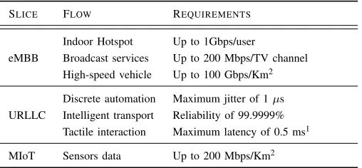
TABLE I: Exemplary 5G traffic requirements.
SLICE FLOW REQUIREMENTS
Indoor Hotspot Up to 1Gbps/user
eMBB Broadcast services Up to 200 Mbps/TV channel High-speed vehicle Up to 100 Gbps/Km2
Discrete automation Maximum jitter of 1µs URLLC Intelligent transport Reliability of 99.9999%
Tactile interaction Maximum latency of 0.5 ms1
MIoT Sensors data Up to 200 Mbps/Km2
1Note: end-to-end maximum delay as defined in [18].
A. Characterization of network traffic and infrastructure
According to the Next Generation Mobile Network Alliance (NGMN) [17], 5G services are expected to be provided via ad-hoc network slices over the same physical infrastructure. In order to enable the desired traffic treatment in the network infrastructure, the 3rd Generation Private Partnership (3GPP) has defined a set of flows with the corresponding traffic requirements for the eMBB and URLLC slices [18], while NGMN in [19] defined the traffic requirements for the MIoT slice. eMBB services are characterized by high bandwidth and span from classical mobile traffic (e.g., mobile terminals), to broadcast-like services (e.g., IPTV), high-speed vehicles (e.g., in-vehicle infotainment), indoor hotspot (e.g., fiber-like access), and dense urban (e.g., crows in a stadium, square). On the contrary, URLLC services are characterized by low latency and span from discrete automation (i.e., remote-controlled robots), to intelligent transport systems (e.g., autonomous cars), and tactile interaction (e.g., augmented reality). Finally, MIoT services are characterized by a high number of inter-mittent and low-power communications (e.g., sensors). Table I reports a selected number of the above traffic requirements as reported in [18], [19].
Based on the different slices and traffic flows introduced above, the authors in [14] first identify three reference de-ployment scenarios, namely urban, industrial, and rural. Next, they characterize the average number of BSs/km2 for each scenario. Specifically, they report for the urban scenario an average number of 72 BS/km2in case of supporting the indoor hotspot traffic flow, which is characteristic of business districts and office areas that require 4 BSs per building floor. In residential/commercial areas instead, the average number of BS/km2 is 12 in urban scenarios. Similarly, 12 BSs are also required in the industrial scenario to satisfy the traffic demand of 1 km2. Finally, the rural scenario considers a 4-lane road (e.g., highway) supporting the intelligent transport system flow (e.g., V2X) and requires 1 BS per kilometer of road.
M1
Base Station 6x Base Stations
per M1 node
6x M1 nodes per access ring
M2 4x access rings
per M2 node
Access ring Aggregation ring
M3 6x M2 nodes per
aggregation ring rings per M3 node2x aggregation
M4
Core
Access Aggregation
Internet Core ring
Fig. 4: Reference network infrastructure as illustrated in [14] and based on [20]
topology point of view, there is no difference whether the BSs are macro, micro, pico, and any variation thereof. For the sake of validating our model, what really matters is the number of BSs and how they are connected to the transport network.
Next, each aggregation ring comprises 6 M2 nodes, each of which serves 4 access rings. In turn, each aggregation ring is served by two M3 nodes for redundancy reasons, while each M3 node provides gateway capabilities to 2 aggregation rings. Finally, M4 nodes are connected to the core ring and serve as gateway to M3 nodes. According to the reference network infrastructure, any of these BSs and M nodes (e.g., M1, M2, M3, and M4) is a good candidate for placing a MEC PoP.
To better understanding which location is most suitable, we need to characterize the RTT. To that end, all the network links are assumed to be fiber optic and are characterized by a propagation delay of 5 µs/km [21]. We also consider a processing delay of 50µs on each of the M nodes [22], [23]. Therefore, the Eq. (26) becomes:
RT T = 2d·5µs
km+ 2M·50µs+U L+DL (28)
where d stands for the distance in kilometers between the MEC PoP and the BS, and M is the number of M nodes (i.e., number of hops) being traversed. For instance, M = 0
in case of collocating the MEC PoP with the BSs, M = 1in case of collocating the MEC PoP with M1 nodes, M = 2
in case of collocating the MEC PoP with M2 nodes, etc. Therefore, the first two terms in the right hand side of Eq. (28) correspond to the propagation delay RTT and the packet processing delay RTT in the transport network, respectively. The last two terms (i.e., UL and DL) correspond instead to the Uplink and Downlink delay over the radio link.
3GPP defines multiple profiles for the radio interface (i.e., New Radio – NR) and each of these profiles is characterized by distinct UL and DL delay values [24]. Bound to the most stringent one-way latency of0.5ms for the tactile interaction URLLC traffic flow (see Table I), the BSs used for the results exposed in Sec.V are 5G gNodeBs with the suitable radio profiles that satisfy U L+DL < RT T = 1ms; hence “BS” refers to a 5G gNodeB from now on. Table II reports the NR profiles used, which all adopt an uplink semi-persistent scheduling (SPS), and the maximum distancesdfrom a BS to a MEC PoP.
TABLE II: NR profiles satisfying the tactile interaction latency
PROFILE DL UL M1
DISTANCE
M2
DISTANCE
FDD 30 kHz 2s 0.39 ms 0.39 ms 12 km 2 km
FDD 120 kHZ 7s 0.33 ms 0.33 ms 24 km 14 km
TDD 120 kHz 7s 0.39 ms 0.39 ms 12 km 2 km
Note: FDD 30 kHz 2s stands for Frequency Division Duplex scheme with a subcarrier of 30 kHz and 2 symbols.
Note: DL and UL values are the worst case transmission latencies presented in [24].
B. Characterization of the deployment areas
Based on the identified urban, industrial, and rural scenarios, we select three reference areas in Spain to apply our model (see Sec. III) and obtain the MEC PoP locations. Specifically, we select Madrid city center for the urban scenario, Cobo Callejaarea for the industrial scenario, andHoces del Cabriel valley for the rural scenario; then we consider the following characterization aspects.
1) Characterization of G(x): before applying the model we characterize each scenario’sgentrification function G(x), revolution functionfi, and population circlesCi. Particularly
fi is based on the smoothstep function, which is derived from Hermite interpolation polynomials [25] and has the following expression:
SN(x) =
0 x≤0
xN+1PN
n=0
N+n n
2N+1
N−n
(−x)n if0≤x≤1
1 if1≤x
(29) more specifically we define fi as:
fi(x) =
0 if kx−cikV >2b+a
Pi if kx−cikV ≤2b
SN 2b+a− kx−cikV if b2<kx−cikV < b2+a
(30) where Pi is the population present in the population circle
Ci with center ci. Therevolution function fi takes the value
Pi in the circle B x,2b
outer disk, D x,b
2,
b
2+a
, where k·kV denotes Vincenty’s
distance [26] using the WGS-84 datum [27].
For Madrid city center we consider as population circles the different districts inside the M-30 ring highway, which administratively identifies the city center and its outskirts. Then, for each of these districts we obtain the Pi, a, bvalues from the city center population census [28]. For what concerns the Cobo Calleja industrial area, around100000people3work daily in the area, and one population circle is enough to cover the 8 km2 region. In Madrid city center and Cobo Calleja, each population circle centerci lies over a LTE tower
retrieved from OpenCellID [30]. Finally, regarding the Hoces del Cabriel rural area, rather than using the population to determine the BSs’ location, we limit our analysis to the location of 1 BS/km [14] along the A-3 highway crossing the rural area.
2) Characterization of BSs’ generation: to generate the BSs’ locations, this work uses the inhomogeneous Mat´ern II point process described in Proposition III.2 together with the average number of BSs described in Sec. IV-A. In the case of Madrid city center and Cobo Calleja areas, we require an average ofE(N(Ri)) = 12BSs/km2 [14]4, which is obtained
by taking x1,s = x2,s = 1 km, r = 2·1km/d
p
(12)e (see
Eq. (25)) andλ(x) =k·G(x), wherek= 16for Madrid city center andk= 13 for Cobo Calleja. These values have been obtained using the average number of points expression that we derive in Proposition III.2.
The urban scenario necessitates additional considerations on the indoor hotspot traffic flow, which is not ubiquitous but rather present at few and specific location in Madrid city center. Following the same approach of [14], we consider the indoor hotspot traffic flow to be present only in office buildings5 which require 4 femtocells on each floor.
On the other hand for Hoces del Cabriel Valley, as men-tioned in Section IV-A, we locate 1 BS/km along the highway to support the intelligent transport system flow. That is, the location and number of BSs follows the route of the highway rather than the population.
3) Characterization of MEC PoPs maximum distances: Al-gorithm 1 uses Eq. (27) to determine the maximum separation between a MEC PoP and a BS. To do so it needs to know the used distance for the propagation delay between a MEC PoP and a BS (i.e., what is dinl(kx−mkd)), and the used
BSs’ NR profile of Table II. Since Sec. IV-A assumes that a BS is connected to a MEC PoP with a fiber link, which are usually installed along the road lanes, Algorithm 1 uses the Manhattan distance, so we havel(kx−mkd) =l(kx−mk1).
Regarding the NR profile, it assumes that all the generated BSs have the same radio technology to have a fixed value of tr = U L+DL in Eq. (27). Hence we need a dedicated execution per NR profile to know how it affects the MEC PoPs’ deployment.
3Estimation based in the number of employees working in Cobo Calleja
companies [29].
4Here we are not considering the indoor hotspot traffic flow for the urban
scenario.
5In this work we consider office buildings with more than 15 floors [31].
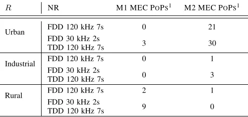
TABLE III: Number of MEC PoPs necessary per NR profile
R NR M1 MEC POPS1 M2 MEC POPS1
Urban FDD 120 kHz 7s 0 21
FDD 30 kHz 2s
TDD 120 kHz 7s 3 30
Industrial FDD 120 kHz 7s 0 1
FDD 30 kHz 2s
TDD 120 kHz 7s 0 3
Rural FDD 120 kHz 7s 2 1
FDD 30 kHz 2s
TDD 120 kHz 7s 9 0
1For Urban and Industrial, average number of MEC PoPs across the 100
simulations.
For sake of clarity, when applying our model to the urban and rural scenarios, it might happen that some of the generated points are not be physically suitable for hosting a gNB (e.g., they fall in the middle of a road). Nevertheless, given the propagation delay of 5 µs/km for fiber optics, a slight misplacement of gNodeBs is negligible since it would only vary the end-to-end delay of few microseconds, which is an order of magnitude smaller when considering an overall latency of milliseconds.
V. SIMULATIONS ANDRESULTS
To obtain the MEC PoP locations we run 100 simulations using R and the spatstat package [32]. Each simulation6 consists of two steps:
1) Generation of 12 BSs/km2using “inhomogeneous Mat´ern II” PPs with the parameters derived from Sec. IV-B2 (in Madrid city center the indoor hotspot BSs are included as well);
2) Generation of MEC PoPs using the NR profiles of Ta-ble II, and Algorithm 1;
For the rural scenario of Hoces del Cabriel valley, we skip step 1) and manually generate 1 BS/km along the A-3 highway that crosses the region. Therefore, we only run step 2) of the simulation to obtain the MEC PoPs needed for the BSs generated across the highway.
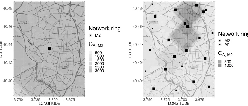
For each scenario only one of the 100 simulations is de-picted in Fig. 5, where we represent the geographical locations of the MEC PoPs as squares or romboids depending on whether they are associated to network ring M2 or M1, re-spectively. Urban, industrial and rural scenarios are illustrated in Fig. 5a, Fig. 5b, and Fig. 5c, respectively; with left and right figures representing how MEC PoP locations vary depending on the used radio technology. A heat map is then used to show the number of BSs CA,M that can be assigned to a MEC PoP at level M. The darkest area in the rhs of Fig. 5b means that any MEC PoP associated to M2 and deployed inside that area has CA,M2=80 BSs whose traffic can be assigned to itself.
The average number of MEC PoPs for each scenario is reported in Table III. Results show that collocating the MEC PoPs with the BSs doesn’t provide enough advantages in terms
6Code available at: https://github.com/MartinPJorge/mec-generator/tree/
40.40 40.42 40.44 40.46 40.48
−3.750 −3.725 −3.700 −3.675
LONGITUDE
LA
TITUDE
Network ring M2
CA, M2
500 1000 1500 2000 2500 3000
40.40 40.42 40.44 40.46 40.48
−3.750 −3.725 −3.700 −3.675
LONGITUDE
LA
TITUDE
Network ring M2 M1
CA, M2 500 1000
(a) Urban scenario (Madrid city center).
40.255 40.260 40.265 40.270 40.275
−3.77 −3.76 −3.75 −3.74
LONGITUDE
LA
TITUDE
Network ring M2
CA, M2 25 50 75 100
40.255 40.260 40.265 40.270 40.275
−3.77 −3.76 −3.75 −3.74
LONGITUDE
LA
TITUDE
Network ring M2
CA, M2 20 40 60 80
(b) Industrial scenario (Cobo Calleja).
39.45 39.50 39.55 39.60 39.65
−1.8 −1.7 −1.6 −1.5 −1.4
LONGITUDE
LA
TITUDE
Network ring M1 M2
CA, M1 20 30 40
50 39.45
39.50 39.55 39.60 39.65
−1.8 −1.7 −1.6 −1.5 −1.4
LONGITUDE
LA
TITUDE
CA, M1 5 10 15 20 25
Network ring M1
(c) Rural scenario (Hoces del Cabriel).
0 0.33 0.66 1
6 20 40 60 80 100 120 144
eC
DF
#radio heads associated to a MEC PoP Industrial (Cobo Calleja)
Urban (Madrid city center) Rural (Hoces del Cabriel)
FDD 120 kHz 7s TDD 120 kHz 7s FDD 30 kHz 2s
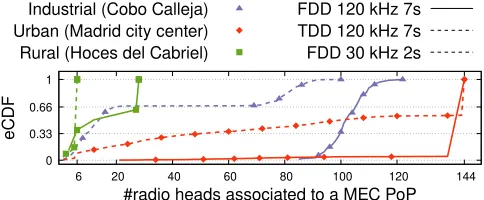
Fig. 6: eCDF of the number of BSs assigned to a MEC PoP in the studied scenarios.
of BSs aggregation and target traffic delay requirement. This is because the network delay (see Eq. (28)) can be satisfactorily fulfilled by aggregating more BSs in fewer MEC PoPs at higher network rings (e.g., M1, M2, etc.). In fact, Algorithm 1 minimizes the number of MEC PoPs whilst fulfilling the traffic requirements. Such traffic requirements (e.g., 1 ms RTT constraint for the URLLC slice) are never satisfied when the MEC PoPs are located at the M3 and M4 network rings, yielding to empty matrices[M3] and matrices[M4]. The reason of such behavior is that packet processing delay (see Eq. (28)) increases linearly with the number of network rings to be traversed. As a result, the MEC PoPs have been always associated to M1 or M2 network rings in all our simulations, as it can be appreciated in one of the simulation realizations shown in Fig. 5.
The lower the packet processing time, the higher the max-imum distance between a BS and a MEC PoP (see Eq. (28)). Thus MEC PoPs associated to M1 have more candidate BSs to be assigned than MEC PoPs associated to M2. But among all the candidate BSs it can only have 6 BSs assigned, while a MEC PoP associated to M2 can have up to 144 BSs assigned. For both the urban and industrial scenarios, the results of our 100 simulations (see Table III) show that most of the MEC PoPs are associated to M2. Since both scenarios have short distances and propagation delays because of the high density of BSs/km2, the addition of M2 packet processing delay does not exceed the 1 ms RTT of URLLC. Therefore, Algorithm 1 associates the MEC PoPs to the M2 network ring, and assigns them as many BSs as possible to reduce the number of MEC PoPs. Conversely, looking to Figure 5c, more MEC PoPs are associated to M1 in the rural scenario because distances and propagation delay to BSs are high enough to exceed the 1 ms RTT when MEC PoPs are associated to M2.
Regarding the different NR profiles (see Table II), low UL and DL delays of FDD 120 kHz 7s permit to increase the maximum distance between a BS and a MEC PoP. Therefore, a MEC PoP can serve a larger number of BSs, as shown in the darker heat maps at the lhs of Fig. 5. As a result, using FDD 120 kHz 7s as NR profile necessitates the deployment of fewer MEC PoPs compared to all the other NR profiles (see Table III). Indeed, any MEC PoP location in the urban and industrial scenario can serve any FDD 120 kHz 7s BSs in the region as shown in Fig. 5a and Fig. 5b. Instead, FDD 30 kHz 2s and TDD 120 kHz 7s impose a higher UL and DL delay,
thus requiring a shorter distance between a BS and a MEC PoP. This results in a larger number of MEC PoPs sparsely located in the region (see rhs of Fig. 5).
Fig. 6 illustrates the experimental Cumulative Density Func-tion (eCDF) for the number of BSs assigned to a MEC PoP. Results show that the FDD 120 kHz 7s NR technology increases the number of BSs associated to a MEC PoP (less than the 33% of them have less than 100 BSs assigned in the industrial and urban scenario), while the other NR technologies lead to a higher percentage of MEC PoPs with fewer BSs assigned. For example, 68% of the MEC PoPs of the industrial scenario have less than 70 BSs assigned when TDD 120 kHz 7s or FDD 30 kHz 2s are used, which is less than half the BSs that can be assigned to a MEC PoP associated to M2.
Summarizing, there is a trade-off between the performance of the NR profile and the number of MEC PoPs. Higher per-formance radio profiles, which can be more expensive, allow to associate a larger number of BSs to a MEC PoP, resulting in fewer MEC PoPs. On the contrary, a less performant radio profile, which is cheaper, requires a large number of MEC PoPs for satisfying URLLC traffic. This trade-off should be taken into consideration by the network operators to optimize costs when building their network.
VI. CONCLUSIONS ANDFUTUREWORK
In this article we have presented a mathematical model to determine the deployment of Base Stations (BSs) and MEC Points of Presence (PoPs), using novel point processes that account for both people population and minimum distances between BSs. The model is applied in real urban, industrial and rural scenarios, where we generate 5G gNodes B and MEC deployments that satisfy the strictest 5G latency constraint of Ultra-Reliable and Low Latency Communications (URLLC) slices, and thus can support future Augmented Reality/Virtual Reality (AR/VR) and low latency streaming services. We have also analyzed the use of 3 future New Radio (NR) profiles of 5G and simulations show that FDD 120 kHz 7s is the technology that minimizes the number of MEC PoPs needed to support the future traffic demands. Future directions of this work include the analysis of the resource requirements of the MEC PoPs, the usage of clustering techniques for the assignment of BSs to MEC PoPs, and the formulation of an optimization problem to minimize MEC PoP deployment costs.
REFERENCES
[1] 3GPP, “System Architecture for the 5G System,” 3rd Generation Part-nership Project (3GPP), Technical Specification (TS) 23.501 v15.4.0, 12 2018.
[2] L. Han, S. Appleby, and K. Smith, “Problem statement: Transport support for augmented and virtual reality applications,” Working Draft, IETF Secretariat, Internet-Draft draft-han-iccrg-arvr-transport-problem-00, March 2017, http://www.ietf. org/internet-drafts/draft-han-iccrg-arvr-transport-problem-00.txt. [Online]. Available: http://www.ietf.org/internet-drafts/ draft-han-iccrg-arvr-transport-problem-00.txt
[4] Y. C. Hu, M. Patel, D. Sabella, N. Sprecher, and V. Young, “Mobile edge computing – A key technology towards 5G,”ETSI White Paper, vol. 11, 2015.
[5] F. Giust, X. Costa-Perez, and A. Reznik, “Multi-Access Edge Comput-ing: An Overview of ETSI MEC ISG,”IEEE 5G Tech Focus, vol. 1, no. 4, 2017.
[6] V. Suryaprakash, P. Rost, and G. Fettweis, “Are Heterogeneous Cloud-Based Radio Access Networks Cost Effective?” IEEE Journal on Selected Areas in Communications, vol. 33, no. 10, pp. 2239–2251, Oct 2015.
[7] A. Baddeley, C. internazionale matematico estivo, and W. Weil, Stochas-tic Geometry: Lectures Given at the C.I.M.E. Summer School Held in Martina Franca, Italy, September 13-18, 2004, ser. Lecture Notes in Mathematics / C.I.M.E. Foundation Subseries. Springer, 2007. [8] V. Suryaprakash, J. Mller, and G. Fettweis, “On the Modeling and
Anal-ysis of Heterogeneous Radio Access Networks Using a Poisson Cluster Process,”IEEE Transactions on Wireless Communications, vol. 14, no. 2, pp. 1035–1047, Feb 2015.
[9] J. Neyman and E. L. Scott, “Statistical Approach to Problems of Cosmology,” Journal of the Royal Statistical Society. Series B (Methodological), vol. 20, no. 1, pp. 1–43, 1958. [Online]. Available: http://www.jstor.org/stable/2983905
[10] A. M. Ibrahim, T. ElBatt, and A. El-Keyi, “Coverage probability analysis for wireless networks using repulsive point processes,” in2013 IEEE 24th Annual International Symposium on Personal, Indoor, and Mobile Radio Communications (PIMRC), Sept 2013, pp. 1002–1007. [11] M. Afshang and H. S. Dhillon, “Poisson cluster process based analysis
of hetnets with correlated user and base station locations,”IEEE Trans-actions on Wireless Communications, vol. 17, no. 4, pp. 2417–2431, April 2018.
[12] M. Syamkumar, P. Barford, and R. Durairajan, “Deployment Characteristics of ”The Edge” in Mobile Edge Computing,” in
Proceedings of the 2018 Workshop on Mobile Edge Communications, ser. MECOMM’18. New York, NY, USA: ACM, 2018, pp. 43–49. [Online]. Available: http://doi.acm.org/10.1145/3229556.3229557 [13] V. Frascolla, F. Miatton, G. K. Tran, K. Takinami, A. D. Domenico,
E. C. Strinati, K. Koslowski, T. Haustein, K. Sakaguchi, S. Barbarossa, and S. Barberis, “5G-MiEdge: Design, standardization and deployment of 5G phase II technologies: MEC and mmWaves joint development for Tokyo 2020 Olympic games,” in2017 IEEE Conference on Standards for Communications and Networking (CSCN), Sept 2017, pp. 54–59. [14] L. Cominardi, L. M. Contreras, C. J. Bcrnardos, and I. Berberana,
“Understanding QoS Applicability in 5G Transport Networks,” in2018 IEEE International Symposium on Broadband Multimedia Systems and Broadcasting (BMSB), June 2018, pp. 1–5.
[15] B. Matern, Spatial Variation, ser. (Meddelanden fr˚an Statens Skogs-forskningsinstitut). Springer New York, 1986.
[16] R. Schneider and W. Weil, Stochastic and Integral Geometry, ser. Probability and its Applications. Berlin, Germany: Springer, 2008. [17] NGMN, “Description of Network Slicing Concept,” Next Generation
Mobile Networks Alliance, White Paper v1.0, 2 2016.
[18] 3GPP, “Service requirements for next generation new services and markets,” 3rd Generation Partnership Project (3GPP), Technical Speci-fication (TS) 22.261, 09 2018, version 16.5.0.
[19] NGMN, “5G White Paper,” Next Generation Mobile Networks Alliance, White Paper v1.0, 2 2015.
[20] ITU-T, “Consideration on 5G transport network reference architecture and bandwidth requirements,” International Telecommunication Union - Telecommunication Standardization Sector (ITU-T), Study Group 15 Contribution 0462, 2 2018.
[21] F. Cavaliereet al., “Towards a unified fronthaul-backhaul data plane for 5G The 5G-Crosshaul project approach,” Computer Standards & Interfaces, vol. 51, pp. 56–62, 2017.
[22] EANTC, “Juniper Networks MPC9E: EANTC Performance, Scale and Power Test Report,” European Advanced Networking Test Center, White Paper v1.0, 4 2016.
[23] ——, “Huawei 5G-Ready SDN: Evaluation of the Transport Network Solution,” European Advanced Networking Test Center, Tech. Rep., 09 2018.
[24] J. Sachs, G. Wikstrom, T. Dudda, R. Baldemair, and K. Kittichokechai, “5G Radio Network Design for Ultra-Reliable Low-Latency Communi-cation,”IEEE Network, vol. 32, no. 2, pp. 24–31, March 2018. [25] R. Burden and J. Faires,Numerical Analysis. Brooks/Cole, Cengage
Learning, 2011. [Online]. Available: https://books.google.it/books?id= KlfrjCDayHwC
[26] T. Vincenty, “Direct and inverse solutions of geodesics on the ellipsoid with application of nested equations,”Survey Review, vol. 23, no. 176, pp. 88–93, 1975.
[27] W3C, “WGS84 Geo Positioning,” 2006.
[28] Padr´on Municipal de Habitantes, “Poblaci´on por distrito y barrio,” http://www-2.munimadrid.es/TSE6/control/seleccionDatosBarrio, 2018, [Accessed: 2018-10-17].
[29] Registro Mercantil y de Bienes Muebles de la Provincia de Madrid, “Registro Mercantil de Madrid,” https://www.rmercantilmadrid.com/RMM/Home/Index.aspx, 2018, [Accessed: 2018-08-27].
[30] “OpenCellID,” http://opencellid.org, 2018, [Accessed: 2018-08-31]. [31] Ministerio de Hacienda, “Sede Electr´onica del Catastro,”
http://www.sedecatastro.gob.es/, 2018, [Accessed: 2018-09-21]. [32] A. Baddeley, E. Rubak, and R. Turner, Spatial Point Patterns:

![Fig. 4: Reference network infrastructure as illustrated in [14] and based on [20]](https://thumb-us.123doks.com/thumbv2/123dok_us/1108580.1611984/7.612.54.561.57.220/fig-reference-network-infrastructure-illustrated-based.webp)