978-3-901882-70-8 c2015 IFIP
Empirical Comparison of Power-efficient Virtual
Machine Assignment Algorithms
Jordi Arjona Aroca
Universidad Carlos III de Madrid, Madrid, Spain Email: [email protected]
Antonio Fernández Anta
Institute IMDEA Networks, Madrid, Spain Email: [email protected]
Abstract—The advent of cloud computing has changed the way many companies do computation, allowing them to outsource it to the cloud. This has given origin to a new kind of business, the cloud providers, which run large datacenters. In order to be competitive, cloud providers must keep the energy consumed by the datacenter low. One way to achieve this is with smart task assignment algorithms, which decide where tasks are to be placed upon their arrival.
In this paper we compare the performance of multiple task assignment algorithms for saving energy. We assume tasks are in fact virtual machines that have to be assigned to physical machines, and we assume that the physical machines have a power consumption that increases superlinearly with the load. Then, we propose an assignment algorithm VMA2 and compare its performance with other state-of-the-art assignment algorithms, both theoretical or already deployed in real cloud computing platforms. VMA2 leads to low energy consumption. It outperforms the other algorithms in most situations, proving itself to be an effective assignment algorithm for cloud computing platforms.
Index Terms—Cloud computing, Datacenters, Virtual Machine Assignment, Energy Efficiency, Scheduling, Load Balancing.
I. INTRODUCTION
Cloud computing has brought a huge number of new solu-tions for problems which were even unknown in the business world. One of these solutions is the possibility of outsourcing large amounts of computation to servers in the cloud and not needing to acquire computers that would be underused and soon outdated. Of course this not only saves money to the companies but also energy, as these servers were usually kept running 24/7 even when they were not being used. However, these costs have been moved to companies, such as Amazon Web Services [1], Rackspace [3], or Citrix [2], specialized in providing computing power. Although these companies make large profits, their principal way of enlarging margins is to increase the efficiency of their servers as much as possible. Virtualization plays, hence, a key role here, minimizing the computational resources that have to be used. However, vir-tualization is like a play with multiple actors, and one of the leading actors in this play are the assignment algorithms.
Assignment (or allocation) algorithms are in charge of deciding to which Physical Machine (PM) is a Virtual Machine
This work has been supported in part by the Regional Government of Madrid (CM) grant Cloud4BigData (S2013/ICE-2894, cofunded by FSE & FEDER), and the Spanish MINECO/MICINN grant TEC2011-29688-C02-01.
(VM)1 assigned upon its arrival. Traditionally, it has been considered that these algorithms were to minimize the number of PMs required to host the number of tasks present in the system. The belief was that using less PMs increases the overall efficiency and reduces the costs in power consumption. This reasoning was due to the fact that, in the past, PMs used to be single core and were not able to change their frequency of operation, what led to a linear dependency between the power consumption and the load.
However, after the arrival of multicore machines the rules have changed. As shown in [4], nowadays, the power con-sumption of data center servers has a superlinear dependency on their load. This non-linear dependency implies the exis-tency of optimal loads and paying higher costs, in terms of power consumption, when PMs are loaded beyond that optimal load. Hence, having superlinear models has a direct effect on the way VMs are assigned as, now, minimizing the number of PMs used might not be the optimal solution anymore. A theoretical study of this problem, a.k.a. the Virtual Machine Assignment Problem (VMA), assuming a superlinear power model is presented in [5], where a competitive analysis of multiple offline and online cases of this problem is provided. This document intends to extend the work of [5] by providing an empirical comparison via simulations of our own devised online algorithms against multiple state-of-the-art assignment algorithms currently used in popular cloud computing platforms such as OpenNebula [12], Koala [6], or Eucalyptus [8]. In addition we propose a new assignment algorithm, VMA2, that leads to low energy consumption. Hence, the main contributions of this paper are two. First, we present VMA2, a novel power aware assignment algorithm. Second, we make a detailed study of two version of the VMA problem, and compare the performance ofVMA2,VMA1 (which we proposed in [5]), and multiple state-of-the-art algorithms in different meaningful scenarios. VMA2 proves itself as a valid assignment algorithm, since it outperforms the other algorithms in most of the cases.
Roadmap. The paper is organized as follows. In Section II we overview related work. Section III describes the VMA problem and the cases that we will analyze, while Section IV introduces our proposed algorithms. Simulations are described
and presented in Section V. We finally present our conclusions in Section VI.
II. RELATEDWORK
The empirical and theoretical work related to VMA is vast and its detailed overview is out of the scope of this paper. We focus on empirical references and refer the reader to [5], and the references therein, to find some theoretical context.
Srikantaiah et al. [13] show that VMA cannot be reduced to a bin packing problem if our goal is an energy efficient assignment. That is, assuming linear energy models and trying to minimize the number of PMs used. Therefore, energy models such as the proposed in [5], where the optimal load of a PM is a function only of the fixed cost of being active (b) and the exponential rate of power increase on the load (α) (that is, the optimal load is not related to the maximum capacity of a PM) seem to be more appropriate. Based on this energy model, we compare, in this work, some of the allocation policies presented in [5], [10] and [11].
Jansen and Brenner [10] evaluate the allocation of VMs to clusters following 9 placement policies, some of them included in popular cloud platforms like OpenNebula [12] or Eucalyptus [8], considering a linear energy cost model. The policies they consider are, namely, Round Robin, Striping, Packing, Load Balancing (free CPU count), Load Balancing (free CPU ratio), Watts per Core, and Cost per Core. We will adapt 5 of these policies to our model and cost function for the purpose of simulations.
Mills et al. [11] provide an objective method to compare different placement algorithms. They perform their analysis using 3different cluster choice criteria and6different alloca-tion heuristics from the bin packing literature, that are used in cloud platforms such as Koala [6] or Eucalyptus [8]. These policies are, namely, First Fit, Least-Full First, Most Loaded First, Next Fit, Random Assignment, and Tag & Pack. We use all these policies, except Tag & Pack, in our simulations.
Finally, Arjona et al. [5] perform a thorough offline and online analysis of multiple cases of the VMA problem. In particular, they consider four different cases defined by whether the number of PMs or their capacity are bounded or unbounded. The main novelty on their study is the already mentioned superlinear energy consumption model and an online allocation algorithm, that we denote asVMA1.
This work extends [5] by providing an empirical analysis comparing the different aforementioned state-of-the-art assign-ment algorithms against VMA1 and a new algorithm that we propose in this work (and that will be denoted as VMA2). Similarly, the main difference between most of the algorithms in [10] and [11] andVMA1andVMA2is that the latter provide power aware assignments while the former do not.
III. THEVMA PROBLEM
The VMA problem is described in [5] as follows. Given a set S ={s1, . . . , sm} of m >1 identical physical machines
(PMs) of capacity C; rational numbers µ, α and b, where µ >0,α >1 andb >0; a setD={d1, . . . , dn} ofnvirtual
machines and a function`:D →Rthat gives the CPU load
each virtual machine incurs, the aim is to obtain a partition π={A1, . . . , Am}ofD, such that(Ai)≤C, for alli. Then,
the objective is minimizing the power consumption given by the function
P(π) = X i∈[1,m]:Ai6=∅
µ X
dj∈Ai
(dj) α
+b
!
. (1)
Based on these definition, the authors describe 4 different cases, (·,·)-VMA, (C,·)-VMA, (·, m)-VMA, and (C, m) -VMA. The difference between these 4 cases lies on whether the capacity and the number of PMs are bounded or not. The results presented in this work are related to the (·, m) -VMA case, where the number of PMs is bounded but not their capacity; and the(C, m)-VMA case, where both the capacity and the number of PMs are bounded.
We also inherit the definition of optimal load, denoted as x∗, as the load at which the power rate, defined as the power consumed per unit of load, is minimized. The optimal load of a PM is given byx∗= (b/(α−1))1/α. We refer the reader to [5] for further details on the description of the problem and the optimal load.
IV. PROPOSEDALGORITHMS
As mentioned in Section II, we want to compare two power aware algorithms,VMA1andVMA2, with several state-of-the-art allocation algorithms. In this section we introduce both algorithms and provide their pseudocode, which can be found in Algorithms 1 and 2.
As can be seen, both algorithms have a certain bin-packing like flavour but including a power awareness aspect, since they do not fill PM up to its maximum capacity but up to its optimal loadx∗. Similarly, both algorithms are similar, being
Algorithm 1:Online algorithmVMA1for(·,·)-VMA and
(C,·)-VMA problems.
for each VMdi do
if(di)>
min{x∗,C}
2 then
di is assigned to a new PM
else
di is assigned to any loaded PMsj where
`(Aj)≤
min{x∗,C}
2 . If such loaded PM does not exist,di is assigned to a new PM.
Algorithm 2: Online algorithmVMA2for the(·,·)-VMA problem.
for each VMdi do
if(di)≥x∗ then
di is assigned to a new PM
else
di is assigned to the PMsj such that
their main difference the threshold imposed on the amount of load per PM, min{x2∗,C} forVMA1andx∗ forVMA2.VMA1, which was already introduced in [5], is able to achieve better competitive and approximation ratios than VMA2. However, theoretical results do not necessarily mean better results in real deployments. In some scenariosVMA2 allows a more packed solution than VMA1, i.e., providing solutions where the load per PM is closer tox∗ than with VMA1. This packing ability might result in a lower power consumption, conditioned by the value of αand on whether the PMs’ capacity is bounded or not.
Both VMA1 and VMA2 have been extended to handle a bounded number of PMs when necessary. This is achieved by assigning the incoming task to the least loaded machine when no more new PMs are available. Similarly, VMA2 has also been extended to deal with the bounded capacity case, when required, by using a threshold of min{x∗, C} and checking whether a new load fits into the targeted PM. In case a new load does not fit, it is assigned to the first possible PM with available resources.
V. EMPIRICALEVALUATION
In this section we evaluate the performance of VMA1 and VMA2 via simulations, and compare them to other state-of-the-art online allocation algorithms.
A. Simulations Setup
The performance of bothVMA1andVMA2is first compared with a lower bound, denoted LBVMA, that is obtained as follows. The input VMs are sorted in non-increasing order of their loads. Then, using this order, as many VMs as possible with load at least x∗ are assigned to different PMs. LetLbe total load of the VMs still unassigned. If there are bL/x∗c
still unused PMs they will be used. Otherwise all PMs will be used. Finally, the load L is assigned among all used PMs as if it could be infinitely divided (i.e., as a fluid), using a water-filling algorithm [7].
We evaluate both(·, m)-VMA and(C, m)-VMA problems. Therefore, in the (C, m)-VMA case a VM can only be assigned to a PM if the latter has sufficient capacity to host it. We test both algorithms VMA1 andVMA2 and also compare them with the following algorithms proposed in the literature:
• Random Fit (RF) [11]: It chooses a PM for each VM uniformly at random among the PM. If the chosen PM cannot allocate the load of the VM, the process is repeated, until the VM is assigned to a PM.
• Next Fit (NF) [11]: Starting initially at the first PM, each new VM is assigned to the next PM after the latest PM to which a VM was assigned (in a cyclic fashion) and with sufficient capacity to host it.
• Least Full First (LFF) [11]: Each new VM is assigned to (one of) the least loaded PM(s) in the system with enough capacity to host it.
• Striping (S) [10]: Each new VM is assigned to (one of) the PM(s) with the smallest number of VMs assigned and with enough capacity to host it.
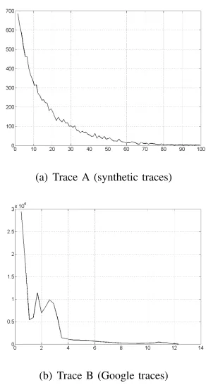
(a) Trace A (synthetic traces)
(b) Trace B (Google traces)
Fig. 1. VMs load distributions used in the evaluations.
• Watts per Core (WC) [10]: Assigns each new VM to the PM whose power would suffer the smallest increase and with enough capacity to host it.
• First Fit (FF) [11]: Each new VM is placed in the first PM that can host it, starting from the first PM.
• Round Robin (RR) [10]: Like FF but, after the first VM is assigned, the search starts from the latest PM in which a VM was allocated.
• Packing (P) [10]: Each new VM is assigned to (one of) the PM(s) with the largest number of VMs assigned provided that the PM can host it.
• Most Full First (MFF) [11]: Each new VM is assigned to the most loaded PM in which it fits.
Observe that, given its nature, First Fit, Round Robin, Packing and Most Loaded First can be only considered for the(C, m)-VMA problem. If PMs had infinite capacity, these algorithms would place all VMs in only one PM. The re-maining algorithms are evaluated for both (·, m)-VMA and
(C, m)-VMA.
The behavior of the aforementioned algorithms is evaluated by inputting the two sets of traces, synthetic and real, shown in Figure 1. We call them Trace AandTrace B, respectively. Trace A is generated by randomly choosing the load of each VM following a power-law distribution with exponential cutoff, which has been chosen so 100% is the maximum task load of a VM. We randomly select 10000 integer loads using this distribution. The loads are inputed in the system sequentially. This leads us to the VM load distribution shown in Figure 1(a).
TABLE I
SIMULATION PARAMETERS FOR A SET OF MACHINES FOR THE
(·, m)-VMACASE.
(·,·)-VMA case
b x∗[GCPS] µ
α= 1.5 α= 2 α= 2.5 α= 3
73.05 10 1.46E-13 7.31E-19 4.87E-24 3.65E-29 92.15 30 3.55E-14 1.02E-19 3.94E-25 1.71E-30 111.25 50 1.99E-14 4.45E-20 1.33E-25 4.45E-31 135.125 75 1.32E-14 2.40E-20 5.85E-26 1.60E-31 159 100 1.01E-14 1.59E-20 3.35E-26 7.95E-32 187.65 130 8.01E-15 1.11E-20 2.05E-26 4.27E-32 206.75 150 7.12E-15 9.19E-21 1.58E-26 3.06E-32 350 300 4.26E-15 3.89E-21 4.73E-27 6.48E-33 541 500 3.06E-15 2.16E-21 2.04E-27 2.16E-33 779.75 750 2.40E-15 1.39E-21 1.07E-27 9.24E-34 1018.5 1000 2.04E-15 1.02E-21 6.79E-28 5.09E-34
extract all the tasks from these traces, assuming that each task is an independent VM. We assume that the VMs (tasks) arrive at the system in the same order at which hey arrived to the Google system, sorting them by the arrival time (given in the trace). The task load of a VM is the maximum CPU load of the task. The trace then contains 124885 VMs with loads varying between 0.31% and 12.5%. The resulting VM load distribution can be seen in Figure 1(b). The load values of the VMs for both distributions are given in percentage in order to scale them up depending on the maximum capacity of a PM in the(C, m)-VMA case or to an appropriate value in the
(·, m)-VMA case.
Each execution of the algorithms is run with a fixed number of PMs. This number of PMs increases from1 to the number of VMs in the trace being used. This allows us to see how the power consumption and how the algorithms behavior evolve when the number of available PMs in the system varies. Finally, in order to evaluate both (·, m)-VMA and (C, m) -VMA, we emulate different PMs by determining their α, b, µ and x∗ parameters as well as the PM maximum capacity or the maximum task load when it corresponds. Then we run the proposed algorithms for each one of these emulated PMs and compare the influence of the different values for these parameters on the final results.
B. Results for (·, m)-VMA
We first evaluate(·, m)-VMA. The first step is to define the set of PMs that we are going to use to evaluate it. To do so, we fix the values ofα,bandx∗and computeµdepending on the previous parameters. In particular, we usedα={1.5,2,2.5,3}
and x∗ = {10,30,50,75,100,130,150,300,500,750,1000}
(given in (Giga)Cycles per Second (GCPS) following the conclusions from [4]). The values of b are determined by interpolation of the baseline costs of Nemesis,Survivor
andErdos, whose values forb (∼85W, 67W and215 W) are known from the experiments performed in [4]. These combinations of parameters result in 44different instances of PMs which are shown in Table I.
Additionally, taking advantage of the fact that the task loads from Trace A and B are given in percentage, and in order to
study the importance of the x∗ to task load ratio, we define the maximum VM load λ as the maximum task load that a VM arriving to the system can have. Therefore, the task load of the VMs arriving to the system will be the product of the task load (in percentage) andλ.
We study three different scenarios. In the first one we study the effect of αfor different values of λand x∗ when using VMA1,VMA2, and the lower boundLBVMA. Second and third scenarios are devoted to compare our proposed algorithms with the state-of-the-art algorithms, always keeping LBVMA as a reference. In the second scenario we study the relevance ofλ while keepingαandx∗ constant. Finally, in the third one, we study the effect of having different values ofx∗ while λand
αremain unaltered.
Scenario 1 compares the power consumed by partitions obtained with VMA1 or VMA2 and for Trace A and Trace B. We compare these results to the ones achieved byLBVMA, that lower bounds the optimal power consumption. The results obtained are presented as graphs in which the power consumed is represented as a function of the number of PMs used.
Figure 2 shows the results for TraceA, for2different values of x∗, 30and300 GCPS, and for 2values of λ, 10and100
GCPS. We can clearly see how the power consumption is smaller for larger values of α once the optimal number of used PMs is reached. This is mainly conditioned by how µ decreases asαincreases (See Table I). Also, as it can be ob-served, there is no qualitative difference in the solutions when αvaries for a given configuration. Due to space limitations we only show a small sample of the results for Trace A, however, similar results are obtained for Trace B as well as for other combinations ofx∗ andλ.
Regarding the performance of the algorithms, we can see how the power consumed by the partitions found withVMA2 is lower, in all cases, than the ones obtained byVMA1and is always closer to the lower bound obtained by LBVMA. This shows that the performance of VMA2 is close to the optimal for (·, m)-VMA. We can see how, in general,VMA1 is able to match the results of VMA2 when the number of PMs is relatively low. However, due to the threshold imposed on the load of the PMs for each algorithm,VMA2is able to pack the load in less PMs. We only find an exception in Figure 2(c), when x∗/λ < 1/3. In this case VMA2 exhibits a behavior relatively similar toVMA1, not being able to hold to its best power consumption and reducing the quality of the solution when the number of PMs increases. However, this flaw is not replicated when using Trace B, where the average task load is smaller.
Scenario 2 compares the performance of LBVMA, VMA1 andVMA2 with the other assignment algorithms proposed in the literature. Here, the values of x∗ and α are fixed to 30
GCPS and 2, respectively, while the value of λ varies. In particular we use λ = {10,30,100} GCPS. Figures 3 and 4 present the results for Trace A and Trace B2.
(a) 10 GCPS,x∗= 30 (b) 10 GCPS,x∗= 300 (c) 100 GCPS,x∗= 30
Fig. 2. (·, m)-VMA: Comparing the power consumed byVMA1andVMA2with the lower boundLBVMAforx∗={30,300}GCPS,α={1.5,2.5}
andλof10GCPS and100GCPS for Trace A (Synthetic traces).
(a)λ= 10GCPS (b)λ= 30GCPS (c)λ= 100GCPS
Fig. 3. (·, m)-VMA: Comparing the power consumed by the different assignment algorithms forx∗= 30GCPS,α= 2andλ={10,30,100}GCPS for
Trace A (Synthetic traces).
(a)λ= 10GCPS (b)λ= 30GCPS (c)λ= 100GCPS
Fig. 4. (·, m)-VMA: Comparing the power consumed by the different assignment algorithms forx∗= 30GCPS,α= 2andλ={10,30,100}GCPS for
Trace B (Google traces).
We can easily see, in general,3 different trends in Figures 3 and 4. The first trend would include LBVMA, VMA1 and VMA2; then we have a second one includingStriping,RF,NF andLLF; and, finally, in some sort of no-man’s land, we have WC. These trends have their origin in power awareness. While LBVMA,VMA1,VMA2andWC are power aware, the rest are not. According to Figures 3 and 4, power aware algorithms outperform the non power aware ones.
It is interesting to see how WC reduces its power con-sumption (for Trace A) as the ratio x∗/λ decreases and even performs better than VMA1 and VMA2 for λ = 100 GCPS. This does not happen, though, for Trace B due to the smaller
average task load, that gives advantage to VMA1and VMA2. With Trace B, due to its nature,WCobtains partitions that use less PMs and hence, because of the superlinear dependence of the power consumption on the load, have higher power consumptions.
task load.
Note also that the non power aware algorithms pay a higher power bill due to the use of a larger amount of PMs (in general) with a smaller amount of load per PM, resulting in a very inefficient usage of the available resources. This behavior is consistent for both Traces A and B.
Finally, observe how the larger the ratiox∗/λ, the larger the gap between our proposed algorithms, VMA1andVMA2, and the other ones. VMA2 exhibits the best results except for the case of Trace A and x∗/λ ∼ 1/3, that implies having tasks whose load is much larger than the optimal load of the system, what should be a rare situation.
Let us now analyze the results of the last scenario. Here we keep λ = 30GCPS and α = 2 constant while we vary the value ofx∗. These results are shown in Figure 5 for Trace A and in Figure 6 for Trace B.
The results are similar for both traces. We can see how for the smallest value, x∗ = 10 GCPS (x∗/λ ∼ 1/3) all algorithms achieve a similar result. As the ratio x∗/λ increases, the results obtained by VMA1 and VMA2 become better than the ones achieved byWC,LLF,NF,Striping, and RF, that increase withx∗ and, therefore, lead to larger power consumptions. Although we do not show them, for the sake of saving space, the figures for x∗ ={30,50,300}, for both traces A and B, would complete this gradual process, being the intermediate steps between the already shown ones. These results are in line with the results from Scenario 2 and are motivated by the fact that the state-of-the-art algorithms tend to use a large amount of PMs keeping its average load low and, hence, paying a high price because of the b parameter. This, however, is not the case of WC, which, on the other hand, obtains a more packed partition, loading PMs beyond x∗ and paying an extra cost due to the superlinearity of the power consumption with respect to the load. Finally, observe that, as happened in Scenario 2, with the exception of the case ofx∗= 10GCPS for Trace A due to the small value ofx∗/λ, VMA2 achieves the best results.
C. Results for (C, m)-VMA
As we did with (·, m)-VMA in Subsection V-B, we start by defining the set of PMs we are going to work with. While for(·, m)-VMA we assumed that PMs had infinite capacity, in
(C, m)-VMA the PMs capacity is bounded. We denote the ca-pacity asC. We define2sets of instances that we name after2
real PMs from our laboratory,NemesisandErdos. We use, as a reference, their maximum capacity,11.2and153.6GCPS; and idle cost b,80and200 W. Jointly with C andb, we use α={1.5,2,2.5,3}, andx∗={0.5,0.65,0.75,0.9,1,1.1} ·C. We can now compute the value of µfor each combination of these4parameters fully defining, then, our set of PMs, which is shown in Tables III and II.
In this case we consider2different scenarios. In the first one we compare againVMA1andVMA2withLBVMAfor different values ofαto evaluate its influence. In the second scenario, we evaluate the performance of VMA1, VMA2, and all the state-of-the-art algorithms whenα,bandCare fixed andx∗varies.
TABLE II
SIMULATION PARAMETERS FOR A SET OF MACHINES WITHbANDC
SIMILAR TOER D O S.
Erdos-like Family Max. Capacityb= 200C= 153W .6GCPS
x∗[GCPS] x∗[%C] µ
α= 1.5 α= 2 α= 2.5 α= 3
76.8 50 1.88E-14 3.39E-20 8.16E-26 2.21E-31 99.84 65 1.27E-14 2.01E-20 4.23E-26 1.00E-31 115.2 75 1.02E-14 1.51E-20 2.96E-26 6.54E-32 138.24 90 7.78E-15 1.05E-20 1.88E-26 3.79E-32 153.6 100 6.64E-15 8.48E-21 1.44E-26 2.76E-32 168.96 110 5.76E-15 7.01E-21 1.14E-26 2.07E-32
TABLE III
SIMULATION PARAMETERS FOR A SET OF MACHINES WITHbANDC
SIMILAR TONE M E S I S.
Nemesis-like Family Max. Capacityb= 80C= 11W .2GCPS
x∗[GCPS] x∗[%C] µ
α= 1.5 α= 2 α= 2.5 α= 3
5.6 50 3.82E-13 2.55E-18 2.27E-23 2.28E-28 7.28 65 2.58E-13 1.51E-18 1.18E-23 1.04E-28 8.4 75 2.08E-13 1.13E-18 8.25E-24 6.75E-29 10.08 90 1.58E-13 7.87E-19 5.23E-24 3.91E-29 11.2 100 1.35E-13 6.38E-19 4.02E-24 2.85E-29 12.32 110 1.17E-13 5.27E-19 3.17E-24 2.14E-29
Note that all simulations are run for both Trace A and Trace B as well as for both families of PMs, however, due to space limitations only the most relevant results are shown. Similarly, observe that results are presented, again, as graphs in which the power consumed is represented as a function of the number of PMs used but, this time, these results do not start from 1
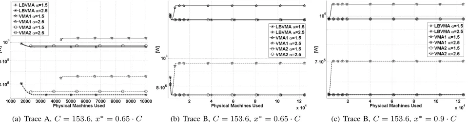
PM. Each one of the results of the different algorithms starts from the number of PMs for which it obtained a valid solution where PMs do not have to be loaded beyond their capacityC. The results for the first scenario, shown in Figures 7, throw very similar results to the ones obtained for (·, m)-VMA. VMA2 performance is again very close to LBVMA when it does not match it. Similarly,VMA1is again worse thanVMA2 due to the fact that it tends to pack less VMs per PM than VMA1. Observe that we show two different values ofx∗ and different Traces to show the consistency of the results.
(a)x∗= 10 (b)x∗= 100 (c)x∗= 500
Fig. 5. (·, m)-VMA: Comparing the power consumed by the different assignment algorithms forλ= 30GCPS,α= 2and increasing values ofx∗for Trace A (Synthetic traces).
(a)x∗= 10 (b)x∗= 100 (c)x∗= 500
Fig. 6. (·, m)-VMA: Comparing the power consumed by the different assignment algorithms forλ= 30GCPS,α= 2and increasing values ofx∗for Trace B (Google traces).
(a) Trace A,C= 153.6,x∗= 0.65·C (b) Trace B,C= 153.6,x∗= 0.65·C (c) Trace B,C= 153.6,x∗= 0.9·C
Fig. 7. (C, m)-VMA: Comparing the power consumed byVMA1andVMA2toLBVMAforx∗={0.65,0.9} ·C,C= 153.6GCPS,α={1.5,2.5}for
Traces A and B.
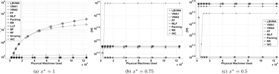
Oppositely to the (·, m)-VMA case, in (C, m)-VMA WC exhibits a better performance than VMA1, that also loses in the comparison with the group of bin-packing-like algorithms formed byFF,MLF,PackingandRRin every case except for Trace A andx∗= 0.5·C, shown in Figure 8(c)3. This worse performance of VMA1 is a consequence of the ability of the other algorithms to obtain more packed solutions whose load is, additionally, closer to x∗ thanVMA1’s solution.
On the other hand, VMA2 results are similar or slightly
3The behaviour shown in Figure 8(c) is not replicated for Trace B because of the smaller average load of Trace B VMs.
worse than FF, MLF, Packing and RR for Trace A when x∗>0.75C (Figure 8(a)). However, VMA2still outperforms the other algorithms whenx∗≤0.75C(Figures 8(b) and 8(c)), or when the average VM task load is smaller, i.e., all the cases of Trace B.
VI. CONCLUSIONS
(a)x∗= 1 (b)x∗= 0.75 (c)x∗= 0.5
Fig. 8. (C, m)-VMA: Comparing the power consumed by the different assignment algorithms forC= 11.2GCPS,α= 2and different values ofx∗for Trace A (Synthetic traces).
(a)x∗= 1 (b)x∗= 0.75 (c)x∗= 0.5
Fig. 9. (C, m)-VMA: Comparing the power consumed by the different assignment algorithms forC= 11.2GCPS,α= 2and different values ofx∗for Trace B (Google traces).
cases of the virtual machine allocation problem, being one of them, (C, m)-VMA, the closest one to real environments. These simulations have been carried out with both synthetic and real traces, being VMA2 results even better with the real ones.
Having outperformedVMA2algorithms which are currently being used in popular cloud platforms, such as Eucalyptus or OpenNebula, we firmly thinkVMA2is ready to be deployed in such or similar platforms, which will be the natural extension to this work.
REFERENCES
[1] Amazon web services. http://aws.amazon.com. Accessed August 27, 2012.
[2] Citrix. http://www.citrix.com. Accessed August 27, 2012. [3] Rackspace. http://www.rackspace.com. Accessed August 27, 2012. [4] Jordi Arjona, Angelos Chatzipapas, Antonio Fernandez Anta, and
Vincenzo Mancuso. A measurement-based analysis of the energy consumption of data center servers. Ine-Energy. ACM, 2014. [5] Jordi Arjona Aroca, Antonio Fernández Anta, Miguel A.
Mosteiro, Christopher Thraves, and Lin Wang. Power-efficient assignment of virtual machines to physical machines. Future Generation Computer Systems, 2015. In press, available at http://dx.doi.org/10.1016/j.future.2015.01.006.
[6] Christian Baun, Marcel Kunze, and Viktor Mauch. The koala cloud manager: Cloud service management the easy way. InCloud Computing (CLOUD), 2011 IEEE International Conference on, pages 744–745. IEEE, 2011.
[7] Stephen Boyd and Lieven Vandenberghe. Convex Optimization. Cam-bridge University Press, New York, NY, USA, 2004.
[8] Eucalyptus. Eucalyptus. http://www.eucalyptus.com/. Accessed January 20th, 2013.
[9] Joseph L. Hellerstein. Google cluster data. Google research blog, January 2010. Posted at http://googleresearch.blogspot.com/2010/01/ google-cluster-data.html.
[10] R. Jansen and P.R. Brenner. Energy efficient virtual machine allocation in the cloud. InGreen Computing Conference and Workshops (IGCC), 2011 International, pages 1–8, 2011.
[11] K. Mills, J. Filliben, and C. Dabrowski. Comparing vm-placement algorithms for on-demand clouds. InProceedings of the IEEE Third International Conference on Cloud Computing Technology and Science, pages 91–98, 2011.
[12] OpenNebula. Opennebula. http://opennebula.org/. Accessed January 20th, 2013.