627
Volume 64 74 Number 2, 2016
http://dx.doi.org/10.11118/actaun201664020627
PREDICTION OF BANKRUPTCY WITH
SVM CLASSIFIERS AMONG RETAIL
BUSINESS COMPANIES IN EU
Václav Klepáč
1, David Hampel
11 Department of Statistics and Operation Analysis, Mendel University in Brno, Zemědělská 1, 613 00 Brno, Czech Republic
Abstract
KLEPÁČ VÁCLAV, HAMPEL DAVID. 2016. Prediction of Bankruptcy with SVM Classifi ers Among Retail Business Companies in EU. Acta Universitatis Agriculturae et Silviculturae Mendelianae Brunensis,
64(2): 627–634.
Article focuses on the prediction of bankruptcy of the 850 medium-sized retail business companies in EU from which 48 companies gone bankrupt in 2014 with respect to lag of the used features. From various types of classifi cation models we chose Support vector machines method with linear, polynomial and radial kernels to acquire best results. Pre-processing is enhanced with fi lter based feature selection like Gain ratio, Chi-square and Relief algorithm to acquire attributes with the best information value. On this basis we deal with random samples of fi nancial data to measure prediction accuracy with the confusion matrices and area under curve values for diff erent kernel types and selected features. From the results it is obvious that with the rising distance to the bankruptcy there drops precision of bankruptcy prediction. The last year (2013) with avaible fi nancial data off ers best total prediction accuracy, thus we also infer both the Error I and II types for better recognizance. The 3rd order polynomial kernel off ers better accuracy for bankruptcy prediction than linear and radial versions. But in terms of the total accuracy we recommend to use radial kernel without feature selection.
Keywords: bankruptcy prediction, classifi cation, feature selection, support vector machines
INTRODUCTION
Retail companies, as well as companies from other domains, are aff ected by various types of risks. Article deals with fi nancial risks and prediction of bankruptcy which is heavily connected to detection of fi nancial issues across time. In previous decades years large number of authors tried to improve techniques for classifi cation of active and bankrupted companies and prediction possibility of this two states. Classifi cation of companies is understood as the distribution of a given set of companies at a fi nite number of sub-groups, in which all of the companies are suffi ciently similar, in the sense of common properties.
Statistical techniques have been commonly used for prediction or classifi cation of business failure. One of the fi rst authors who used these techniques was Beaver (1955), Altman (1968) who
used multivariate discrimination analysis (MDA), Ohlson (1980) with logit model, Zmijewski (1984) with probit model. Review of selected key works in this fi eld gives Aziz and Dara (2004), who have summarized large portion of diff erent models even like neural networks (NN) and its accuracy in bankrutpcy prediction.
Min and Lee (2005) tested the accuracy of classifi ers on the set of 1888 companies, using the classifi cation by means of NN, MDA, logit and SVM with RBF kernel. The last mentioned approach led to achieving the accuracy 83% on the testing data set which consisted of 20% of all original data. It was the highest accuracy compared with other alternatives which were able to achieve a bit less than 80% accuracy.
Ding, Song and Zen (2008) proposed the model of prediction of fi nancial distress via the application SVM which used 11 fi nancial indicators and data of 250 Chinese companies from the time period 2001–2004. The performance effi ciency of this model was compared with conventional statistic methods (MDA, logit) and with NN. Authors highlighted both the problem of overtraining and diffi cult determination of all parameters of network. The proposed model, when compared with other approaches, achieved the highest predictive performance, i. e. the classifi cation accuracy 83%. It surpassed all the other methods whose accuracies did not show any statistically signifi cant diff erences.
Niknya, Darabi and Vakili (2013) evaluated models for prediction of fi nancial distress via SVM, MDA and logit, using companies at Tehran stock exchange in the time period 2007–2013. They used indicators of activity, profi tability and conversions on one share and divided data into a training and a testing data set, out of which 112 companies were in fi nancial distress and 548 companies were healthy ones. Their survey led to the conclusion that SVM model had the highest classifi cation capability – 93%, logit model achieved the 85% accuracy and MDA only 82%.
Shin, Lee and Kim (2005) applied SVM and three-fold neural network (NN) in bankruptcy prediction. They used the data of 2230 Korean production companies (in the time period 1996–1999) with the ratio 50:50 between fi nancially bankrupted and fi nancially healthy companies. They used feature selection from MDA and t-test of indenpendence, to reduce initial 250 variables to only 10 variables. The conclusion of this testing was that the usage of SVN was more advantageous for a smaller training set (around 50 companies), which did not apply to NN (hundreds of companies) where it was more diffi cult to fi nd optimal parameters. The overall accuracy when data sets of various size were compared was between 80–90% for the training data set and 80% for NN.
Min, Lee and Han (2006) proposed predictive performance of SVM, NN and logistic regression on the case of prediction of bankruptcy. Furthermore, they suggested the method of the choice of input characteristics and optimalization of SVM parametres using genetic algorithms. The measurement was carried out on real data of 614 Korean production companies, out of which 307 bankrupted in the time period 1999–2002. The bankruptcy was predicted on the basis of various data sets of variables with the count 32,
30, 12 and 6. The highest classifi cation accuracy 80.3% was achived when using model GA-SVM with 32 variables and it was the highest accuracy compared with other models. Logistic regression achieved only 68% accuracy – the same as for NN.
For the data of bankruptcies of 250 publicly traded Chinese companies, Dong et al. (2008) used SVM method and other methods (NN, logit and MDA) for bankruptcy prediction. These results proved that model SVM with RBF kernel to be the most advantageous. The accuracy of clasifi cation via SVM was 95.2% for training and 83.2% for testing data set. The method of NN led to the worst results – 76% on the testing data set.
Motivation and Contributions
The main aim of this paper is to test the prediction accuracy of SVM methods with diff erent kernel types and diff erent lag of data. Practically, we want to fi nd out if it is possible to predict bankruptcy 1–5 years ahead with solid accuracy and obtain comparable results to previous studies. On the basis of above stated we want to benchmark prediction abilities of diff erent SVM based models especially for linear and non-linear kernel types (3rd order polynomial and Radial basis kernels).
We approach and partly replicate research steps in Min and Lee (2005) in the case of SVM application. Similarly to the work of Shin, Lee and Kim (2005) this paper uses feature (attribute) selection procedures in order to obtain non-reduntant attributes with informative value. The results enhance literature with at least one main contribution concerning research studies about retail business fi eld: assessing of the best SVM model and its kernel types which are useful for the prediction of bankruptcy and inference of Error I and II. In preparing steps of the analysis we classify and summarize facts about retail business companies in EU which can be used for more specifi c research, especially concerning fi nancial risk of retail businesses. We used data from retail medium-sized companies, when other authors mostly used data of big manufacturing companies or fi nancial institutions. In results we concentrate to SVM classifi cation models with respect to particular feature selection methods, which in our best knowledge, ain’t been conducted before in that form.
MATERIAL AND METHODS
Liquidity ratio, Solvency ratio, Sales). Subsequent data analysis steps were performed in so ware R 3.1.1.
Selection of appropriate features plays essential role in data mining because it helps to identify the best variables to capture unique variability of data set. Feature selection (FS) reduces the dimensionality of feature space, and removes redundant, irrelevant, or noisy data. According to Jain and Zongker (1997) selection techniques broadly falls into two categories: wrapper and fi lter methods. In this paper we concern only fi lter method.
Feature selection brings the immediate eff ects for application: speeding up an algorithm, improving the data quality and thereof the performance of classifi er. In the case of the fi lter methods the subset selection procedure is independent of the learning algorithm and is generally a pre-processing step. Methods evaluate the relevance of the predictors outside of the models and subsequently uses only the predictors that pass some criterion. Only predictors with important relationships would then be included in a classifi cation model. Filters are based on some importance measure which is independent from many classification method, such as for example correlation between features and decision class or information gains. We use Relief algorithm, Chi-squared fi lter, Gain ratio which are incorporated into R package. Technical details about these fi lter methods can be found in Kononen (1994), Quinlan (1993), Tsai (2009) or Holčík (2012).
Representations of Binary SVM Models Binary SVM is a linear classifi er that maximizes the margin between the separating hyperplane and the training data points. The hyperplane is based on a set of training data which lie closest to the boundary and are called support vectors. The algorithm implicitly maps the input data in the feature space, and an inner-product induced in the algorithm is calculated by kernel functions without
considering the feature space itself. The SVM problem is expressed by a quadratic programming optimization problem with linear constraints, see Vapnik (1995). For this reason, the SVM always produces global solution for classifi ers. The SVM is an unique supervised learning algorithm that o en achieves superior generalization performance compared to other learning algorithms across most domains and tasks.
The algorithm can automatically determine a network architecture. It is less sensitive to the curse-of-dimensionality and more robust to a small number of high dimensional samples than other non-SVM classifi ers. Application domains typically have involved high-dimensional input space, and the good performance is also related to the fact that SVM’s learning ability can be independent of the dimensionality of the feature space. With training set D = {xiti}
N
i=1 with input vector, xi = (xi
(1), K, x
i
(n))T Rn
and labels ti {−1, 1} and K what is kernel function, we could describe SVM classifi er according to Vapnik’s formulation
ti[t(x
i) + b] ≥ 1, i = 1, …, N,
where represents the weight vector and b the bias. The non-linear function (.): Rn Rnk maps the input or measurement space to a high-dimensional, and possibly infi nite-dimensional, feature space. We defi ne optimization problem
1
1 ( , )
2
N T
i i
MinJ c
subject to: ti(
t(x
i) + b) ≥ 1 − i ,i = 1, …, N.
i≥ 0, i = 1, …, N.
Variables i are slacks we need to allow
misclassifi cations in the set of inequalities. C R+ is a tuning hyperparameter, weighting the importace I: Median for all variables (from 2009 to 2013 for active and bankrupted companies)
Variable median/Year 2009 2010 2011 2012 2013 Active Ban. Active Ban. Active Ban. Active Ban. Active Ban.
Total assets (EUR) 1617123 2593634 1818387 2469198 1951387 2625785.5 2094287 2263953.5 2140751 1418862 Working capital (EUR) 69388.5 65559 82401 28945.5 80783 224901.5 119535 13891.5 138060 −128 Sales (EUR) 4841577 3664370 5204420 3283544 5502780 3144102 5704412 2869630.5 5802521 1548052 EBIT (EUR) 73791 28856 81548 5374 79062 5135 73758 −85984 77095 −235767
Collection period (days) 7 10 8 9 8 10 8 6 7 7
Credit period (days) 30 99 29 97,5 30 91 29 112 28 101
Current ratio 1.29 1.19 1.29 1.27 1.3 1.27 1.32 1.18 1.33 0.77
Liquidity ratio 0.5 0.46 0.5 0.47 0.5 0.53 0.5 0.35 0.5 0.22
Solvency ratio (%) 28.11 7.45 28.81 5.73 29.31 4.84 29.42 1.4 31.22 −14.04
WC/TA 0.07 0.1 0.07 0.15 0.07 0.24 0.09 0.05 0.07 0
EBIT/TA 0.05 0.02 0.05 0.01 0.04 0.01 0.04 −0.07 0.04 −0.23
Sales/TA 2.72 1.83 2.82 1.78 2.74 1.46 2.73 1.68 2.71 1.53
of classifi cation errors. We obtain solution of the optimization problem a er constructing the Lagrangian. From the conditions of optimality we obtain quadratic problem in the Lagrange multipliers i. Instances of data corresponding
to non-zero i are called support vectors. Due to
Mercer’s condition, which relates the mapping function (xi) to a kernel function K(·, ·)
K(xi, xj) = (xi)T(x j).
There are three common kernel function types of SVM such as linear kernel
K(xi, xj) = xi
Tx
j
and non-linear kernel types like polynomial
K(xi, xj) = tanh(xixj
T + r)d, where > 0,
is the degree of the polynomial kernel, and radial basis kernel (RBF) defi ned for > 0 as
K(xi, xj) = exp(−1/
2(x
i − xj))
2, for > 0,
where 2 is the bandwidth of the radial basis function kernel. Finaly we construct classifi er
1
( ( , ) )
N
i i i j i
Y sgn y K x x b
,where Y is the output. The details of the optimatization problem are discussed in Chang and Lin (2004) or Vapnik (1995).
Measuring of Prediction Acurracy Standard method how to evaluate the results of classifi cation/prediction is to use confussion matrix like in Tab. II. This matrix could be possibly used for all of the data set parts (training, validation and testing sample) but we evaluate more closely just testing sample.
According to Fawcet (2004) we calculate:
• Sensitivity,what is the proportion of actual positives which are correctly identifi ed as such:
TP =
(TP + FN)
Sensitivity .
• Specifi city, what is the proportion of negatives which are correctly identifi ed as such:
TN =
(FP + TN)
Specificity .
• Classifi cation accuracy is the average rate of accuracy bound both classifi cation labels and Type I and II errors are used for more specifi c accuracies evaluation:
TP TN TP FP FN TN
Accuracy
.
• Empirical Error I evaluates the number of true positives which were classifi ed as true negatives:
FN TP FN Type I Error
.
• In contrast, Empirical Error II shows how many of true negatives were labeled false positives:
FP FP TN
Type II Error
.
Based on these calculated data, the analysis of predictional ability of classifi cation methods via the construction of so-called Receiver Operator Characteristics (ROC) curves can be carried out. This method enables to visualise and analyse the behaviour of diagnostic systems both in medicine and in economic applications. It can be claimed to be a tool for evaluation and optimalization of binar classifi cation system which shows the relation between specifi city and sensitivity of the given test or detector for all allowable values of threshold. The value AUC is the most common index describing the ROC curve, which is suitable for comparison of various classifi cation models where the whole ROC curve is reduced into one scalar quantity with the usual value between 0.5 and 1:
• from 0.50 to 0.75 – eligible, • from 0.75 to 0.92 – good, • from 0.92 to 0.97 – very good, • from 0.97 to 1.00 – perfect.
Technically, the area under the ROC curve is equal to the probability that a classifi er will rank a randomly chosen positive instance higher than a randomly chosen negative example. It measures the classifi ers ability in ranking a set of patterns according to the degree to which they belong to the positive class, but without actually assigning patterns to classes. AUC has a connection with the Gini coeffi cient Gini = 2AUC-1. There is also a large number of papers, for the case of ROC curves, and its enhancements, like is presented in Michálek, Sedlačík and Doudová (2005).
II: Confussion matrix (in our case T is an active company and F signs bankrupted)
Current category
Predicted category
T F
Research Steps
We partly replicate following steps from Shin, Lee and Kim (2005):
• Dividing data set onto particular training, validation and testing (prediction) groups. In this case we want to test accuracy for random samples with 30/30/40 as for training/validation/test partitioning.
• Pre-processing of variables: scaling [0, 1] and removing of correlated variables (over 80% of corelation index).
• Feature selection for 5 most important attributes (to get simplifi ed model) with diff erent fi lter types: Gain ratio, Relief algorithm, Chi-squared fi lter. For comparisson is also used full set with all of the features.
• Training and validation on data and prediction whereas target labels are Bankruptcy or Activity in year 2014.
• Accuracy diagnostics with AUC values and total accuracy evaluation.
• Evaluation of Empirical Error I and Empirical Error II values in case of the best fi tting year with respect to AUC values, to compare with other empirical studies.
RESULTS
The above shown Tab. I illustrates that companies diff er more signifi cantly in its fi nancial indicators no sooner than two or three years before bankruptcy, when the value of assets is gradually decreasing, followed with the drop of company’s liquidity and the growth of indebtedness. One year before bankruptcy, companies start facing distinct fi nancial diffi culties, however their rectifi cation is highly improbable. In reverse, active companies have been
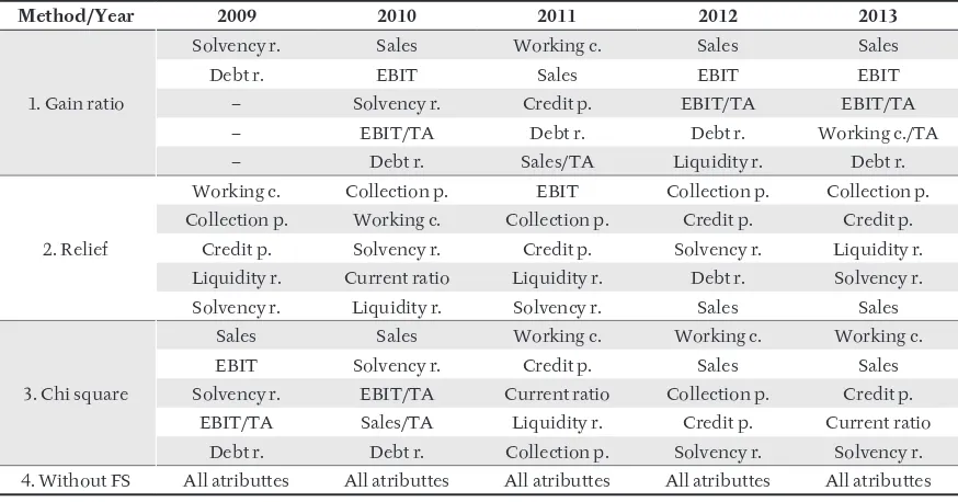
showing similar fi nancial indicators in the fi eld of retail business for all years. In the case of using of fi lters, presented features in the Tab. III are used for the year given.
As can be seen from the comparison of feature selection methods, the classifi cation should incorporate features like Sales, Solvency ratio, Debt ratio. Features like Liquidity ratio or Sales/TA support us with only limited information value.
Evaluation of Prediction Accuracy
A er feature selection, models are constructed and its classifi cation accuracy is carried out for various types of kernels and various settings of ratios of training, validation and testing phase. In Figs. 1 and 2, the total results of accuracy of classifi cation can be seen. They are stated via the value AUC and Accuracy for testing sample, which were based on data of 850 companies in each year.
Fig. 1 illustrates the longer time period till bankruptcy the lower the prediction ability of models is, i.e. fi nancial indicators or real situation for previous years do not refl ect the resulting fi nancial diffi culties on the satisfactory level, or companies have not faced these problems yet. The highest prediction ability can be observed no sooner than in 2013, i.e. one year before bankruptcy. Evaluation via the value AUC is also problematic. Models for lagged data with longer lags provide only low percentage of appropriately classifi ed bankruptcies; technically the diff erences between active companies and those which bankrupt in the future are not as obvious.
The results show that the highest values of the accuracy of classifi cation can be observed mostly in 2013. The diff erence between values can be observed mostly for AUC values, because the total accuracy in years 2009 to 2011 is biased as
III: Selected features by according to its importance
Method/Year 2009 2010 2011 2012 2013
1. Gain ratio
Solvency r. Sales Working c. Sales Sales
Debt r. EBIT Sales EBIT EBIT
– Solvency r. Credit p. EBIT/TA EBIT/TA
– EBIT/TA Debt r. Debt r. Working c./TA
– Debt r. Sales/TA Liquidity r. Debt r.
2. Relief
Working c. Collection p. EBIT Collection p. Collection p. Collection p. Working c. Collection p. Credit p. Credit p.
Credit p. Solvency r. Credit p. Solvency r. Liquidity r. Liquidity r. Current ratio Liquidity r. Debt r. Solvency r. Solvency r. Liquidity r. Solvency r. Sales Sales
3. Chi square
Sales Sales Working c. Working c. Working c.
EBIT Solvency r. Credit p. Sales Sales
Solvency r. EBIT/TA Current ratio Collection p. Credit p. EBIT/TA Sales/TA Liquidity r. Credit p. Current ratio
the models undervalue during the prediction of frequency of bankrupted companies.
It is appropriate to add that models are able to notice correct labels for active companies, however, the longer time period to bankruptcy is, the worse the results are, or the results are inconsistent for bankrupted companies which have been active till now. The polynomial kernel of the third order is showing worse results especially when compared with RBF kernel.
In Tab. IV are shown the Empirical Error I and Empirical Error II type for better recognition of. We use all kernels, which is according to previsous results mostly suitable for evaluation. Thus we can see that results can be fl awed due to the total
accuracy, we need to estimate Error I type and Error II type also. Error I evaluates the number of active companies which were classifi ed as bankrutped. In contrast, Error II type shows how many bankrupted companies were wrongly labeled as active ones. For the purposes of risk prediction, this metric is the key one. That is why the setting of the model with the lowest values is searched. The comparison of variants leads to the clear conclusion, that the best results in the group of kernels is provided by polynomial of 3rd order kernel with Gain ratio based feature selection. This result is not evident from the basic comparison in Fig. 1 and Fig. 2.
1: Evaluation of prediction accuracy and AUC for different SVM kernels (left panels show total acurracy, right panels show AUC, legend signs different years)
DISCUSSION
The main contribution or article lies in concerning statistically evaluated attributes and diff erent kernels for classifi cation a prediction of bankruptcy: diff erent fi lters off er similar results in terms of Type II errors. Most suitable features are Sales and Solvency ratio. This means, that these features have good ability to classify companies in heavier fi nancial distress or even bankrupted across time. Total accuracy of classifi cation is higher than obtained results from previous studies mentioned
in Aziz and Dar (2006) which used logit, neural networks or probit. For the previous application of SVM for bankruptcy prediction are obtained accuracies on the similar level, see Niknya, Darabi and Vakili (2013). But this holds only for total accuracy. With concentration on the Error I and II types, what is essential in bankruptcy prediction, we could add that misclassifi cation rates are very high, especially several years before bankruptcy. We consider that analysis based on diff erent data set proportions or higher number of bankrupted companies in data sets could support us with better results.
SVM methods off er many technological possibilities, especially for modelling of multi-stage credit or default events which should be mentioned in other research. Feature selection, techniques for detecting variables with best informative value for classifi cation is very promissing due to the fact that it off ers simplifi cation of the models. Obviously the obtained results could be further enhanced via testing of accuracy for diff erent kernels and diff erent proportions of training/validation/testing set. We could even test accuracy of diff erent classifi ers like boosted trees or neural networks, like in Min, Sung-Hwan, Lee and Han (2006) or Ding, Song and Zen (2008). SVM and its application in Czech republic is really scarce, there have been no renowned studies with this connection so far. This means that we can perform more SVM based classifi cation concerning Czech data as well.
IV: Evaluation of prediction quality according to Error I and Error II in 2013
Kernel Type I Error Type II Error
Linear without FS 0.014 0.571 Polynomial without FS 0.017 0.643 RBF without FS 0.000 0.786 Linear with Relief 0.016 0.563 Polynomial with Relief 0.022 0.688 RBF with Relief 0.022 0.563 Linear with Gain ratio 0.028 0.500 Polynomial with Gain ratio 0.016 0.375 RBF with Gain ratio 0.000 0.688 Linear with Chi-square 0.019 0.625 Polynomial with Chi-square 0.022 0.688 RBF with Chi-square 0.022 0.500
CONCLUSION
This contribution deals with the application of bankrupty prediction models and its testing when estimating overall prediction accuracy and Area under curve of each model based on SVM method. The main aim of this paper is to test the prediction accuracy of SVM methods with diff erent kernel types with diff erent lag of data. Practically, we want to fi nd out if it is possible to predict bankruptcy 1–5 years ahead with sound accuracy. Data based on Amadeus database consists of accouting values from 2009 to 2013. Our analysis uses data of 802 active retail medium-sized companies and 48 companies which reported bankruptcy in 2014.
Proposed total accuracies are on the same levels as in comparable studies. The variant comparison of models with diff erent models led us to the conclusion that SVM classifi er based on RBF kernel performs well for capturing total accuracy, especially for the formation 1 year ahead prediction. However, this does not apply for evaluation of Type I and II errors – models have signifi cant diffi culties in capturing real bankruptcy or distressed profi le, which holds true especialy for active companies. For a longer period before bankruptcy models are not effi cient enough to predict the bankruptcy – active companies are assigned with bankrupty labels. For this sake and to treat Error II types is better to utilize SVM classifi er with 3rd order polynomial kernel.
Acknowledgement
The paper was supported by the Internal Grant Agency FBE MENDELU under project: Testování modelů pro vícerozměrnou analýzu a predikci kreditního rizika (No. 19/2015).
REFERENCES
ALTMAN, E. I. 1968. Financial ratios, discriminant analysis and the prediction of corporate bankruptcy. The Journal of Finance, 23(4): 589–609. AK, J. and ZONGKER, D. 1997. Feature selection:
Evaluation, application and small sample
performance. IEEE Transactions on Pattern Analysis Machine Intelligence, 19(2): 153–158.
AZIZ, M. A. and DAR, H. A. 2006. Predicting corporate bankruptcy: where we stand? Corporate Governance:
DING, Y., SONG, X. and ZEN, X. 2008. Forecasting fi nancial condition of Chinese listed companies based on support vector machine. Expert Systems with Applications, 34(4): 3081–3089.
HOLČÍK, J. 2012. Analýza a klasifi kace dat. Brno: Akademické nakladatelství CERM.
MIN, J. H. and LEE, Y. C. 2005. Bankruptcy prediction using support vector machine with optimal choice of kernel function parameters. Expert Systems with Applications, 28: 603–614.
KONONENKO, I. 1994. Estimating attributes: Analysis and extensions of RELIEF, in Machine Learning. Lecture Notes in Computer Science, 784: 171–182.
MICHÁLEK, J., SEDLAČÍK, M. and DOUDOVÁ, L. 2005. A comparison of two parametric ROC curves estimators in binormal model. In: Proceedings of the 23rd International Conference Mathematical methods in Economics 2005. Hradec Králové: GAUDEAMUS Univerzita Hradec Králové, 256– 261.
MIN, S.-H., LEE, J. and HAN, I. 2006. Hybrid genetic algorithms and support vector machines for bankruptcy prediction. Expert Systems with Applications, 31(3): 652–660.
NIKNYA, A., DARABI, R. and VAKILI, F. 2013.
Financial Distress Prediction of Tehran Stock Exchange Companies Using Support Vector Machines. European Online Journal of Natural and Social Science, 2(3).
SHIN, K. S., LEE, T. S. and KIM, H. J. 2005. An application of support vector machines in bankruptcy prediction model. Expert Systems with Applications, 28(1): 127–135.
TSAI, C. F. 2009. Feature selection in bankruptcy prediction. Knowledge-Based Systems, 22(2): 120– 127.
OHLSON, J. A. 1980. Financial ratios and the probabilistic prediction of bankruptcy. Journal of Accounting Research, 18(1): 109–131.
QUINLAN, J. R. 1993. Programs for Machine Learning. Morgan Kaufmann Publishers.
VAPNIK, V. M. 1995. The Nature of Statistical Learning Theory. New York: Springer.
ZMIJEWSKI, M. 1984. Methodological issues related to the estimation of fi nancial distress prediction models. Journal of Accounting Research, 22: 59–86.
Contact information Václav Klepáč: xklepac@node.mendelu.cz