5552 IJSTR©2020
Sample Size Estimation In Cohort Studies For
Testing Of Relative Risk
Subramanian Chandrasekaran, Jayadevan Sreedharan, Aji Gopakumar
Abstract: Cohort study is one of the epidemiological research designs to determine incidence rate and risk associated with the health outcome. The study identifies the risk factors of the outcome variable by estimating relative risk (RR) and test of hypothesis about RR. Determining an adequate sample size (n) with sufficient subjects is an important step in any research for generalization of the sample results. This paper discusses a method for calculating adequate sample size in a cohort study, specifically to test the ‘significance of RR in a regression model’. The formula proposed in this paper includes significance level (α), power (1-β), degree of effect to be detected (RR) and desired precision. Simulation is carried out to evaluate the performance of the proposed sample size formula in deriving adequate ‘n’.
Index Terms: Adequate sample size, epidemiological design, cohort study, relative risk, incidence rate, precision, logistic regression model.
—————————— ◆ ——————————
1.
INTRODUCTION
Determination of sample size is an important step in any research. Calculation of adequate sample size leads to inclusion of sufficient number of study subjects to detect significant effect size and facilitate valid generalization of sample results to the whole population. There is different sample size formulas derived according to the design of the study and statistical techniques that expected to apply [1], [2]. Cohort study is one of the observational studies in Medical research, aims to estimate the incidence rate and test the significance of risk ratio. In this design, a cohort is selected on the basis of exposure status as exposed/unexposed. Incidence is measured by regular follow up of the cohort for a period of time. The study involves large number of subjects for a long period of time according to the exposure and outcome of interest. A cohort study is generally carried out after exploring a hypothesis which is strengthened from quicker studies such as cross sectional or case-control studies. The choice of the cohort for a research specifically depends upon the investigated hypothesis and the population has been initially surveyed to explore the presence of exposure. Cohort studies are more suitable if the research is related to an exposure which is rare. In case of rare exposure, lesser number of people may be exposed to the factor and therefore study population consists of deliberate selection of larger exposed group (/highly exposed). As an involvement of large number of subjects in the research, variety of common exposures in relation to several health outcomes can be studied in cohort studies. A similar kind of comparison group is required to be chosen including the participants who are ‘unexposed’ or ‘exposed at low level’ to an exposure understudy [3], [4], [5]. Cohort studies are mainly of two types, prospective and retrospective studies.
In prospective cohort studies, information on exposure will be
collected at present and hence large number of people should be followed up for longer period of time from exposure to disease onset. In retrospective cohort studies, information on exposure will be available from the existing authentic records and consequently time to wait for effect (risk of disease) may be reduced / eliminated. As the focus of cohort studies is follow up till the development of the disease (/multiple outcomes), researchers ensure absence of outcome at entry level. But it may not be ensured all the time, especially in conditions with long latent period and those cases get excluded from the research. Similarly, subjects are often removed from the study for various reasons and hence cohort size should be adequately collected taking all these points into consideration. Exposure effect is measured using Relative Risk (RR) or Risk Difference considering equal/unequal follow-up duration. In order to calculate the exposure effect (RR), incidence needs to be measured among exposed and unexposed; then comparison to be done across the groups. In order to derive valid conclusion, recruitment of sufficient and representative sample is a vital step prior to initiation of any kind of research. Results of the study may mislead if size of the sample is inadequate, however each steps in research are appropriate. Both very large and small samples fail to identify significance of real effect, hence calculation of adequate number of subjects needs to be calculated according to the type of statistical test and study design [6], [7], [8]. Cohort studies generally aim the comparison of exposed and unexposed groups in terms of incidence of health outcome. Objective of this paper is to derive a new formula for adequate sample size in a cohort study. Studies reported that sample size formula (n) for testing of RR in a cohort study includes the factors such as significance level (α), power (1-β), number of control subjects per experimental subjects (m), incidence rates (p1 & p2) among exposed and
unexposed group [9], [10]. A study with estimation of RR doesn’t need to include power term (Zβ) in its sample size formula, but it is necessarily to be included if the purpose of the study is to test a hypothesis related to RR.
2
EXISTING
METHOD
OF
SAMPLE
SIZE
CALCULATION
IN
COHORT
STUDIES
Since selection of sample in a cohort study is based on exposure status, study will be initiated with two groups such as exposed and unexposed; RR will be the parameter of interest
___________________________________
• Subramanian Chandrasekaran is a PhD holder (Statistics) and Associate Professor of Dept. of Statistics, Annamalai University, India. PH-+919715263275. E-mail: [email protected]
• Jayadevan Sreedharan has double PhD in Biostatistics and Epidemiology, Professor of Dept. of Community Medicine, Gulf Medical University, UAE. PH-+9710796101. E-mail: [email protected]
• Aji Gopakumar is a Research Scholar, currently pursuing PhD under the Dept. of Statistics, Annamalai University, India. PH- +9710992363. E-mail:
[11], [12]. The null hypothesis for the test of RR can be expressed as H0: RR=1. Null hypothesis indicates that event rate is same among exposed and unexposed group. In other words, the proportion of disease is same across exposed and unexposed groups. Therefore the null hypothesis can also be written as H0: P1=P2 against the two tailed alternative hypothesis H1: P1≠P2. Here P1 and P2 are the incidence rates among exposed and unexposed group respectively. Implies, the test of hypothesis about RR is equivalent to test of two sample proportions [13]. Since RR is the risk ratio to be detected and P2 the disease rate among unexposed, both are generally known in most cases. Therefore P1 can be expressed as P1= (RR) P2. The existing formula for determining sample size in two-sided test of RR is given as follows [14], [15]
𝑛 = [𝑍1−𝛼/2√2𝑝(1 − 𝑝) + 𝑍1−𝛽 √[𝑝1(1 − 𝑝1) + 𝑝2(1 − 𝑝2)] 2
[𝑝1− 𝑝2]2
Where p= (p1+p2)/2 and the constraint 0 < RR < 1/P2
Z (1-α/2) is the standard normal variate at the chosen level of
significance (z=1.96 and 2.58 at 5% and 1% level of significance respectively) and Z(1-β) is the power term which
commonly fixed at 80%.
3 PROPOSED
SAMPLE
SIZE
FOR
COHORT
STUDY
Theoretically, sample size (n) is the ratio of standard deviation (SD) to the standard error (SE),
𝑛 =𝑆𝐷2
𝑆𝐸2 --- (A)
The current study interested to focus on the simple regression model and the sample size required for finding association between the response variable and one predictor variable which are dichotomous. The corresponding logistic model can be expressed in the following function,
y= e
xβ
1+ exβ
where eβ is the relative risk (risk ratio).
In reference to Confidence Interval (CI) of the parameter of interest, CI can be expressed as
CI = (estimate) ± (Critical value) (SE of the estimate)
where (Critical value x SE of the estimate) is considered as the margin of error (L).
In a cohort study, investigator’s interest is to test the significance of Relative Risk (risk ratio). Hence the confidence interval for the relative risk can be expressed in the following notation, eβ ± Z(α/2)SE (eβ) …………..….(1)
Since we have relative risk and its standard error as follows, Relative risk, eβ=p
1/p2 = (incidence rate among exposed
group)(incidence rate among unexposed group) Implies, Log eβ=Log p
1/p2
Standared Error of (𝐿𝑜𝑔 𝑒𝛽) = √1 − 𝑝1 𝑛1𝑝1
+ 1 − 𝑝2 𝑛2𝑝2
SE of (𝛽) = √1 − 𝑝1
𝑛 𝑝 +
1 − 𝑝2
𝑛 𝑝
L = 𝑍𝛼 2 SE (𝛽)
̂
= 𝑍𝛼 2 √
1−𝑝1
𝑛1𝑝1+
1−𝑝2
𝑛2𝑝2 = 𝑍 𝛼 2 √
1 𝑛(
1−𝑝1
𝑝1 +
1−𝑝2
𝑝2 ) with an
assumption of n=n1=n2
√𝑛 = 𝑍𝛼
2
⁄ √(1−𝑝1𝑝1+ 1−𝑝2𝑝2 )
𝐿 ………….…….. (2)
Since margin of errror represents shift from the true estimate, denominator of equation (2) can be represented as difference in the disease rate (p1-p2)
√𝑛 = 𝑍𝛼
2
⁄ √(1−𝑝1𝑝1+ 1−𝑝2𝑝2 )
𝑝1−𝑝2 ………...(3)
Since the null hypothesis tested in a cohort study is H0: RR=1
(or H0: p1=p2), an equivalent hypothesis can be expressed as
H0: p1-p2=0 against H1: p1-p2≠0
If the null hypothesis is true (under H0), the upper 100(α/2)th
percent point of the distribution of p which centered at 0 can be espressed as
a = 0 + 𝑍𝛼
2√2𝑝(1 − 𝑝)/𝑛 …………..(4)
the distribution if the alternative hypothesis is true (at H1 where
distribution centered at p1-p2),
a = (p1-p2) - 𝑍𝛽√𝑝1(1 − 𝑝1)/𝑛 + 𝑝2(1 − 𝑝2)/𝑛
𝑎 + 𝑍1−𝛽 SE(p1-p2) = p1-p2 ……….(5)
when expression of equation (4) substituted in equation (5), we will get
𝑍𝛼
2√2𝑝(1 − 𝑝)/𝑛 + 𝑍𝛽 √𝑝1(1 − 𝑝1)/𝑛 + 𝑝2(1 − 𝑝2)/𝑛 = 𝑝1− 𝑝2
………..(6)
From equation 3, we have 𝑝1− 𝑝2= 𝑍𝛼
2
⁄ √(1−𝑝1𝑝1+ 1−𝑝0𝑝0 )
√𝑛
while substituting for p1-p2 in equation (6), we get
𝑍𝛼√2𝑃′(1 − 𝑃′)/𝑛 + 𝑍𝛽 √ 1
𝑛[𝑝1(1 − 𝑝1) + 𝑝2(1 − 𝑝2)]
𝑍𝛼 2 ⁄ √(
1 − 𝑝1
𝑝1 +
1 − 𝑝2
𝑝2 )
= 1 √𝑛
Devide both sides by 1 √𝑛 1 1 √𝑛√𝑛 = 1
√𝑛[𝑍𝛼√2𝑃′(1 − 𝑃′) + 𝑍𝛽 √[𝑝1(1 − 𝑝1) + 𝑝2(1 − 𝑝2)]] 1
√𝑛 𝑍𝛼⁄2 √( 1 − 𝑝1
𝑝1 +
1 − 𝑝2
𝑝2 )
√𝑛 = 𝑍𝛼√2𝑃′(1 − 𝑃′) + 𝑍𝛽 √[𝑝1(1 − 𝑝1) + 𝑝2(1 − 𝑝2)] 𝑍𝛼
2 ⁄ √
1 𝑛(
1 − 𝑝1
𝑝1 +
1 − 𝑝2
𝑝2 )
𝑛 = [𝑍𝛼√2𝑃′(1 − 𝑃′) + 𝑍𝛽 √[𝑝1(1 − 𝑝1) + 𝑝2(1 − 𝑝2)]] 2 [𝑍𝛼 2 ⁄ √ 1 𝑛(
1 − 𝑝1
𝑝1 +
1 − 𝑝2 𝑝2 )]2
𝑛 = [𝑍𝛼√2𝑃′(1 − 𝑃′) + 𝑍𝛽 √[𝑝1(1 − 𝑝1) + 𝑝2(1 − 𝑝2)]] 2
(𝑃𝑟𝑒𝑐𝑖𝑠𝑖𝑜𝑛)2
is the adequate sample size required to test the significance of RR in a cohort study. Formula includes p1 and p2 which are the
5554 power respectively. RR is the required relative risk to be
detected.
Precision can be defined as,
Precision = [Standard Normal Variate] x [Standard Error] p1 = (RR) p2 and p =𝑝0+𝑝1
2
Hypothesis about the relationship or causation can be proven with the help of a cohort study, which is considered as the best method of causation (Grimes & Schulz, 2002). Current research paper introduced a sample size formula which is derived by taking both ‘inferential techniques and study design’ into consideration.
4 SIMULATION
RESULTS
4.1 Simulation Results with Existing Sample Size Formula In order to observe the performance of proposed sample size formula, simulation is carried out and various trails were performed for different values of significance level and power. For comparison, minimum sample size for the test of RR is calculated by the existing method in Table 1. ‘n’ is calculated for fixed level of significance (α=0.05), power (80%) and different values of P2. Calculated sample size is presented in the table 1 according to the RR to be detected.
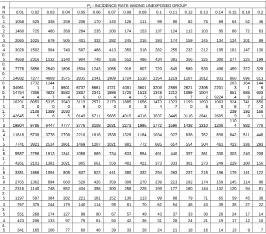
4.2 Simulation Results by the Proposed Method of Sample Size
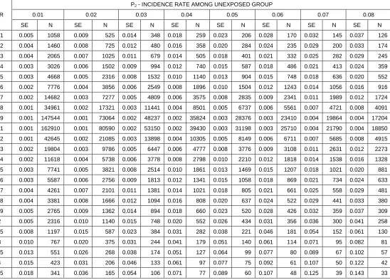
To verify the accuracy of proposed sample size formula, sample size is calculated at different values of precision as well as various disease rates among the unexposed group (p2). Level of significance and power has fixed for varied disease rates and precision. In order to find ‘n’ for different levels of precision, SE can be identified from previous studies which is then multiplied with the Z score. Repeated trials were performed for different power values and significance levels in accordance with the RR to be detected. Simulation results revealed that lesser samples are required to detect larger RR and for higher incidence rates. The findings agree with the theoretical concept of requirement of larger samples to detect a subtle exposure effect. Adequate sample size is presented in table 2 for α level 0.05, 1-β at 0.80 and various values of p2 (0.01-0.2). Precision is calculated at various values of Standard Error (SE) which is multiplied with Z score (table 2-4). From tables 1-4, proposed sample size gives an adequate large ‘n’ in a cohort study to follow up for longer period of time. Since the calculation consists of precision that required for valid inferential statistics, comparatively a better large ‘n’ is reflected as adequate sample size for different values of standard error.
5 CONCLUSION
Sample size proposed in this research is calculated for the desired precision of the estimate; it is considered as the allowable or acceptable error in the estimate. Adequate sample size depends on how precise an investigator needs his descriptive and inferential statistics. Precision has an important role for the estimation of statistics; accordingly marginal of error is fixed for determination of sample size. Hence major components which are affecting the precision are margin of error and confidence level. The proposed sample size formula calculates adequate sample size considering these two major components. An adequate large sample reduces the margin of error and subsequently increase the precision; Confidence level ensures the results found are accurate within this
margin of error. Compared to the size obtained from existing method, the sample size proposed in this study gives an adequate larger sample considering the required precision.
ACKNOWLEDGMENT
The authors would like to acknowledge Annamalai University, India and Gulf Medical University, UAE for the support
provided to conduct this research as a part of PhD completion.
REFERENCES
[1] M.A. Pourhoseingholi, M. Vahedi and M. Rahimzadeh, “Sample size calculation in medical studies,” Gastroenterol Hepatol Bed Bench, vol. 6, no. 1, pp. 14-7, 2013.
[2] P. Dattalo, Determining sample size: Balancing power, precision and practicality. Oxford University Press Inc, New York, 2008.
[3] S.I. Dos Santos, Cancer Epidemiology: Principles and methods. International Agency for Research on Cancer, World Health Organization, ISBN: 978-92-832-0405-3, 1999.
[4] D. Barrett and H. Noble, “What are cohort studies?” Evidence-Based Nursing, vol. 22, no. 4, pp. 95-96, 2019. [5] H. Liu, Y. Shen, J. Ning, and J. Qin. “Sample size
calculations for prevalent cohort designs,” Stat Methods Med Res., vol. 26, no. 1, 280–291, 2017.
[6] C.J. Mann, “Observational research methods. Research design II: cohort, cross sectional, and case-control studies,” Emergency Medicine Journal, vol. 20, no. 1, pp. 54-60, 2003.
[7] C.J. Mann, “Observational research methods––Cohort studies, cross sectional studies, and case–control studies,” African Journal of Emergency Medicine, vol. 2, no. 1, pp. 38-46, 2012.
[8] Centre for Evidence-Based Medicine (CEBM). “Study Designs”. 2014. Retrieved from
https://www.cebm.net/2014/04/study-designs/
[9] V. Kasiulevičius, V. Sapoka, R. and Filipavičiūtė, “Sample size calculation in epidemiological studies”. Gerontologija; vol 7, no. 4, pp. 225–231, 2016.
[10]J. Charan and T. Biswas, “How to Calculate Sample Size for Different Study Designs in Medical Research?” Indian Journal of Psychological Medicine, vol. 35, no. 2, pp. 121-126, 2013.
[11]P.M. Bernard, C. Lapointe, “Calculation of sample size for the detection of relative risk with a predetermined confidence level and power”. Rev Epidemiol Sante Publique, vol. 38, no. 3, pp. 255-60, 1990.
[12]K.J. Lui, “Exact equivalence test for risk ratio and its sample size determination under inverse sampling,” Stat Med., vol. 16, no. 15, pp. 1777-86, 1997.
[13]H. Wang and S.C. Chow. “Sample size calculation for comparing proportions,” 2nd Ed., Chapman and Hall/CRC,
New York, 2007.
[14]S. Lemeshow, D.W. Hosmer and J. Klar, “Sample size requirements for studies estimating odds ratios or relative risks”. Stat Med., vol. 7, no. 7, pp. 759-64, 1988.
TABLE 1: SAMPLE SIZE BY EXISTING FORMULA FOR FIXED VALUES OF α=0.05, 1-β=0.80 AND INCIDENCE RATE
AMONG UNEXPOSED GROUP (P2)
R R
P2 - INCIDENCE RATE AMONG UNEXPOSED GROUP
0.01 0.02 0.03 0.04 0.05 0.06 0.07 0.08 0.09 0.10 0.11 0.12 0.13 0.14 0.15 0.18 0.20
0.1 962 478 316 236 187 155 132 115 101 90 82 74 68 63 58 47 42
0.2 1339 665 440 328 261 216 184 160 141 126 114 103 95 87 81 66 58 0.3 1907 947 627 467 371 307 261 227 200 179 161 147 135 124 115 94 83 0.4 2811 1396 924 688 546 452 384 334 295 263 237 216 198 182 169 137 122 0.5 4358 2163 1431 1065 846 699 595 516 455 407 367 333 305 281 260 211 187 0.6 7293 3618 2393 1781 1413 1168 993 862 760 678 611 556 508 468 433 351 311 0.7 13824 6855 4532 3371 2674 2209 1878 1629 1435 1280 1153 1048 959 882 816 661 583 0.8 33034
1637 4
1082
1 8044 6378 5267 4474 3879 3416 3046 2743 2491 2277 209
4 193
5 156
5 138
0 0.9
13984 5
6928 5
4576 5
3400 5
2694 9
2224 5
1888 5
1636 5
1440 5
1283 7
1155 4
1048 5 9581
880 5
813 3
656 5
578 1 1.1
15523 2
7683 2
5069 9
3763 2
2979 2
2456 5
2083 2
1803 2
1585 4
1411 2
1268 7
1149 9
1049 4
963 2
888 5
714 3
627 2 1.2 40728
2014 8
1328
8 9858 7800 6428 5448 4713 4141 3684 3309 2998 2734 250
8 231
2 185
4 162
6 1.3 18953 9371 6177 4580 3622 2983 2526 2184 1918 1705 1531 1386 1263
115 8
106
6 853 747 1.4 11140 5505 3626 2687 2124 1748 1480 1278 1122 997 894 809 737 675 621 496 433 1.5 7435 3672 2418 1791 1414 1163 984 850 745 662 593 536 488 447 411 327 285 1.6 5376 2653 1746 1292 1020 839 709 612 536 476 426 385 350 320 294 234 203 1.7 4105 2025 1332 985 777 638 539 465 407 361 323 292 265 242 222 176 153 1.8 3262 1608 1057 781 616 506 427 368 322 285 255 230 209 191 175 138 120 1.9 2671 1316 865 639 503 413 348 300 262 232 208 187 170 155 142 112 97 2 2240 1103 724 534 421 345 291 250 219 193 173 156 141 128 118 92 80
2.5 1164 571 374 275 216 176 148 127 110 97 87 78 70 63 58 45 38
3 748 366 239 175 137 111 93 80 69 60 54 48 43 39 35 26 22
3.5 539 263 171 125 97 79 66 56 48 42 37 33 29 26 24 17 14
4 415 202 131 95 74 60 49 42 36 31 27 24 21 19 17 12 10
5556
TABLE 2: ADEQUATE SAMPLE SIZE FOR FIXED VALUES α=0.05, 1-β=0.80, AND VARYING PRECISION & P2
(PROPOSED METHOD)
R R
P2 - INCIDENCE RATE AMONG UNEXPOSED GROUP
0.01 0.02 0.03 0.04 0.05 0.06 0.07 0.08 0.09 0.1 0.11 0.12 0.13 0.14 0.15 0.18 0.2 0.
1 1058 525 348 259 206 170 145 126 111 99 90 82 75 69 64 52 46
0.
2 1460 725 480 358 284 235 200 174 153 137 124 112 103 95 88 72 63 0.
3 2065 1025 679 505 401 332 282 245 216 193 174 159 145 134 124 101 89 0.
4 3026 1502 994 740 587 486 413 359 316 282 255 232 212 195 181 147 130 0.
5 4668 2316 1532 1140 904 748 636 552 486 434 391 356 325 300 277 225 199 0.
6 7776 3856 2549 1896 1504 1243 1056 916 807 720 649 589 539 496 459 372 328 0.
7 14682 7277 4809 3575 2835 2341 1989 1724 1518 1354 1219 1107 1012 931 860 696 613 0.
8 34961 1732
1 1144
1 8501 6737 5561 4721 4091 3601 3209 2889 2621 2395 2201 203
3 164
1 144
5 0.
9
14754 4
7306 4
4823 7
3582 4
2837 6
2341 0
1986 4
1720 4
1513 5
1348 0
1212 6
1099 7
1004 2 9224
851 4
685 9
603 2 1.
1
16291 0
8059 0
5315 0
3943 0
3119 8
2571 0
2179 0
1885 0
1656 3
1473 4
1323 7
1199 0
1093 5
1003 0
924 6
741 7
650 2 1.
2 42645 2108
5 1389
8 1030
5 8149 6711 5685 4915 4316 3837 3445 3118 2841 2605 239
9 192
0 168
1 1.
3 19804 9786 6447 4777 3776 3108 2631 2273 1995 1772 1590 1438 1310 1200 110
4 882 770 1.
4 11618 5738 3778 2798 2210 1818 1538 1328 1164 1034 927 838 762 698 642 511 446 1.
5 7741 3821 2514 1861 1469 1207 1021 881 772 685 614 554 504 461 423 336 293 1.
6 5587 2756 1813 1341 1058 869 734 633 554 491 440 397 361 330 303 240 208 1.
7 4261 2101 1381 1021 805 661 558 481 421 373 333 301 273 249 229 180 156 1.
8 3381 1666 1094 808 637 522 441 380 332 294 263 237 215 196 179 141 122 1.
9 2765 1362 894 660 520 426 359 309 270 239 213 192 174 159 145 114 98 2 2316 1140 748 552 434 356 300 258 225 199 177 160 144 132 120 94 81 2.
5 1197 587 384 282 221 181 152 130 113 99 88 79 71 65 59 45 38
3 767 375 244 179 140 114 95 81 70 62 54 48 43 39 35 27 22
3.
5 551 268 174 127 99 80 67 57 49 43 37 33 30 26 24 17 14
4 423 206 133 97 75 61 50 42 36 31 28 24 21 19 17 12 10
4.
TABLE 3: ADEQUATE SAMPLE SIZE FOR FIXED VALUES OF Α=0.05, 1-Β=0.80, AND VARYING P2 & SE (PRECISION=Z
SCORE X SE)
RR
P2 - INCIDENCE RATE AMONG UNEXPOSED GROUP
0.01 0.02 0.03 0.04 0.05 0.06 0.07 0.08
SE N SE N SE N SE N SE N SE N SE N SE N
5558 TABLE 4: ADEQUATE SAMPLE SIZE FOR FIXED VALUES OF α=0.05, 1-β=0.80, AND VARYING P2 & SE (PRECISION=Z
SCORE X SE)
RR
P2 - INCIDENCE RATE AMONG UNEXPOSED GROUP
0.09 0.1 0.11 0.12 0.13 0.14 0.15 0.18 0.2
SE N SE N SE N SE N SE N SE N SE N SE N SE N
0.1 0.041 111 0.046 99 0.051 90 0.055 82 0.060 75 0.064 69 0.069 64 0.083 52 0.092 46 0.2 0.037 153 0.041 137 0.045 124 0.049 112 0.053 103 0.057 95 0.061 88 0.073 72 0.082 63 0.3 0.032 216 0.036 193 0.039 174 0.043 159 0.046 145 0.050 134 0.054 124 0.064 101 0.071 89 0.4 0.028 316 0.031 282 0.034 255 0.037 232 0.040 212 0.043 195 0.046 181 0.055 147 0.061 130 0.5 0.023 486 0.026 434 0.028 391 0.031 356 0.033 325 0.036 300 0.038 277 0.046 225 0.051 199 0.6 0.018 807 0.020 720 0.022 649 0.024 589 0.027 539 0.029 496 0.031 459 0.037 372 0.041 328 0.7 0.014 1518 0.015 1354 0.017 1219 0.018 1107 0.020 1012 0.021 931 0.023 860 0.028 696 0.031 613 0.8 0.009 3601 0.010 3209 0.011 2889 0.012 2621 0.013 2395 0.014 2201 0.015 2033 0.018 1641 0.020 1445 0.9 0.005 15135 0.005 13480 0.006 12126 0.006 10997 0.007 10042 0.007 9224 0.008 8514 0.009 6859 0.010 6032 1.1 0.005 16563 0.005 14734 0.006 13237 0.006 11990 0.007 10935 0.007 10030 0.008 9246 0.009 7417 0.010 6502 1.2 0.009 4316 0.010 3837 0.011 3445 0.012 3118 0.013 2841 0.014 2605 0.015 2399 0.018 1920 0.020 1681 1.3 0.014 1995 0.015 1772 0.017 1590 0.018 1438 0.020 1310 0.021 1200 0.023 1104 0.028 882 0.031 770 1.4 0.018 1164 0.020 1034 0.022 927 0.024 838 0.027 762 0.029 698 0.031 642 0.037 511 0.041 446 1.5 0.023 772 0.026 685 0.028 614 0.031 554 0.033 504 0.036 461 0.038 423 0.046 336 0.051 293 1.6 0.028 554 0.031 491 0.034 440 0.037 397 0.040 361 0.043 330 0.046 303 0.055 240 0.061 208 1.7 0.032 421 0.036 373 0.039 333 0.043 301 0.046 273 0.050 249 0.054 229 0.064 180 0.071 156 1.8 0.037 332 0.041 294 0.045 263 0.049 237 0.053 215 0.057 196 0.061 179 0.073 141 0.082 122 1.9 0.041 270 0.046 239 0.051 213 0.055 192 0.060 174 0.064 159 0.069 145 0.083 114 0.092 98