6427
Effect of Foreign Direct Investment and
Economic Growth on CO2 Emmision in
Indonesia
Sebastiana Viphindrartin, Herman Cahyo Diartho, Siti Aisah
Abstract: Economic growth and capital movements have risen in the world, this has led to several debates about environmental degradatio n caused.
Carbon dioxide emissions are a form of environmental degradation caused by economic activities. The analytical method used is descriptive analysis method and quantitative analysis method. Descriptive analysis method aims to describe the dynamics that occur in each variable studied. Quantitative analysis in the form of Dynamic Ordinary Least Squares (DOLS) aims to determine the effect of FDI, economic growth, and energy consumption on carbon dioxide emissions. This study uses secondary data from 1981 to 2014. The results obtained are FDI, economic growth, and energy consumption affecting carbon dioxide emissions in Indonesia. The role of the economic sector in regulation of carbon dioxide emissions tends to be significant Index Terms: FDI, Economic Growth, CO2 Emissions, Energy Consumption, DOLS
————————————————————
1 I
NTRODUCTION economic theories, especially growth in the context of macroeconomics, largely ignore environmental problems. Implicitly it is often assumed that the consequences associated with environmental problems are a simple problem and will be resolved by itself (Arrow et al., 1995). Economic growth has undergone a transformation, this is due to the effect of global economic shocks that have a major influence and require the country's economy to be able to keep up with the flow of changes caused. The crisis in 1997/1998 and the global financial crisis in 2008/2009 had a significant impact on the weakening of several important sectors, including the industrial sector and the trade sector. The decline in the existence of the industrial and trade sectors results in the level of energy consumption used (Plummer, 2009). Economic growth is a goal to be achieved by a country, but in achieving a high level of growth will sacrifice the environment, in other words environmental degradation plays an important role in determining the economic growth of a country (Lau et al., 2014). The relationship among environmental degradation and economic growth is based on the Environmental Kuznets Curve (EKC) hypothesis, which states that there is a U-shaped inverse relationship between the level of per capita income and the level of income equality. Therefore, there is a threshold level of economic growth beyond further improvement which is then able to improve the environmental impact caused from the initial stages of economic development (Kizilkaya, 2017). Economic growth that pays attention to environmental impacts is based on a concept of sustainable development. Many ideologies agree that economic development will lead to a trade off between economic and ecological interests. In relation to economic growth in the context of sustainable development, there is an underlying theory, namely Pollution Hypothesis, which is divided into Pollution Haven Hypothesis and Pollution HaloHypothesis which states that there are interrelating relationships between Foreign Direct Investment and environmental pollution. In this view, the investor country that carries out Foreign Direct Investment has more energy efficiency, high technology and management skills (Kizilkaya, 2017). Thus, FDI contributes to a clean environment and further leads to the reduction of greenhouse gas emissions in developing host countries (Zarsky, 1999). While economic growth and capital movements have risen in the world, this has led to several debates about environmental degradation caused. In order to attract FDI with the aim of increasing economic growth, developing countries have ignored environmental problems by implementing loose environmental regulations. Therefore foreign companies prefer to invest in developing countries because they apply fewer taxes and environmental regulations, consequently FDI will cause environmental degradation problems in developing countries. This is called Pollution Haven Hypothesis (Kizilkaya, 2017).
In the current era of globalization, multinational companies can take part and develop throughout the world (Ravenhill, 2014: 3). Countries that are more enthusiastic about increasing their economic growth must use more energy to compensate for higher levels of production and overcome the increasing public demand for energy after rising income levels (Sadorsky, 2010). In order to overcome the increasing demand for energy along with the current environmental problems, it is necessary to change energy use. Therefore, ways to increase cleaner and more sustainable energy use, or what is known as renewable energy, are important things to do.
As a developing country, Indonesia is included in the Newly Industrialized Countries criteria. Changes towards Newly Industrialized Countries (NICs) are offset by changes in GDP output as one of the macroeconomic indicators. In addition to the ongoing economic growth, the standard of living of the people also continues to improve.
Other economic achievements also show that Indonesia has been successful in terms of economic development. This success was despite the problem of the economic crisis in 1997/1998, which caused not only internal mismanagement or policy failure, but also contagion effects from Thailand. The Indonesian economy has moved in a stable direction since 2000 or two years after the 1997/1998 economic crisis. Since then, Indonesia has experienced a moderate, stable and
M
————————————————
Sebastiana Viphindrartin is Lecturer of Economic Development, Economics and Business Faculity, Jember University, Indonesia. E-mail: sebastiana@unej.ac.id
Herman Cahyo Diartho is Lecturer of Economic Development, Economics and Business Faculity, Jember University, Indonesia.E-mail:
hermancahyo.feb@unej.ac.id
Siti Aisah is Student of Economic Development, Economics and Business Faculity, Jember University, Indonesia.E-mail:
stable economy. Along with the increasingly brilliant economic performance, Indonesia was slowly able to get out of the IMF loan scheme at the end of 2003. Thus, the burden of sustainable development will increase along with increasing economic growth.
The role of the economic sector in regulation of carbon dioxide emissions tends to be significant. Regulatory regulation of economic activities is expected to reduce the effects of carbon dioxide emissions produced, but on the other hand these regulations must go hand in hand, with the aim, of economic activities.
This study has a purpose, among others, namely knowing how the influence of FDI and economic growth on carbon dioxide emissions in Indonesia, and knowing the dynamics of the relationship of FDI, economic growth, energy consumption, and carbon dioxide emissions in Indonesia.
2
E
MPIRICAL LITERATUREThe empirical study that deals with the relationship between FDI, economic growth, and CO2 emissions generally addresses the Environmental Kuznets Curves theory, Pollution Halo Hypothesis and Pollution Haven Hyphotesis theory. In this regard, many studies analyze the validity of this hypothesis in various perspectives and countries.
Studies related to EKC are based on the Grossman and Kuruger (1991) hypotheses. In 1991 Grossman and Krueger developed the concept of Simon Kuznets (1955) which was popularized as Environmental Kuznets Curve (EKC), where they applied the Kuznet hypothesis to determine the relationship between economic growth and environmental quality. The EKC theory forms a reversed U-curve that is relevant for various pollutants at higher income levels. While related to the pollution hypothesis theory originated from Copeland and Taylor's hypothesis in 1994 in his research entitled North-South Trade and the Environment. In their hypothesis they state that when trade is liberalized, polluting industries tend to shift from rich countries to strict environmental regulations to poor countries with weak environmental regulations.
Some studies related to the literature include: Kizilkaya (2017) evaluating the relationship between carbon dioxide emissions, economic growth, foreign direct investment and energy consumption in Turkey during the period 1970-2014. Long-term estimation results show that economic growth and energy consumption have a positive impact on CO2 emissions. However, this study did not find a significant relationship between foreign direct investment and CO2 emissions. Omri et al (2014) explored the relationship between energy consumption, income, inflows of foreign direct investment (FDI) and CO2 emissions in Turkey, for the period 1974-2011, stating that the Environmental Kuznets (EKC) and pollution halo hypothesis were supported in Turkey .
Ozturk and Os (2016) apply this empirical model to 3 regional sub-panels: Europe and Central Asia, Latin America and the Caribbean, and the Middle East, North Africa, and sub-Saharan Africa. The results provide evidence of two-way causality between FDI inflows and economic growth for all panels and between FDI and CO2 for all panels, except Europe and North Asia. The hypothesis shows the existence of unidirectional causality that runs from CO2 emissions to economic growth, with the exception of Middle East, North Africa, and sub-Saharan panels, where two-way causality
between these variables cannot be denied. Sbia et al (2014) tested variable unit properties with structural damage. The ARDL boundary testing approach is applied to check cointegration by accommodating structural damage originating from the series. The VECM Granger causality approach is also applied to investigate causal relationships between variables. It was found that foreign direct investment, trade openness and carbon emissions reduce energy demand. Clean economic growth and energy have a positive impact on energy consumption. Linh and Lin (2014) examined the dynamic relationship between CO2 emissions, energy consumption, FDI and economic growth for Vietnam in the period 1980 to 2010 based on the Environmental Kuznets Curve (EKC) approach, cointegration, and Greanger causality tests. The results of the cointegration test and Granger causality show a dynamic relationship between CO2 emissions, energy consumption, FDI, and economic growth. A shorter two-way relationship between Vietnamese income and FDI inflows implies that an increase in Vietnam will attract more capital from abroad. Whereas Brown (2013), focuses on the impact of Foreign Direct Investment (FDI) on the environment. This study identifies FDI, GDP per capita and the capital-labor ratio as the main determinant of CO2 emissions in West Africa. The magnitude of the adverse composition and beneficial scale effects of FDI more than compensates for the benefits of the beneficial technical effects and thus makes FDI damaging carbon dioxide emissions and hence damaging the environment. Lee, Jung Wan (2013) on the results of his tests showed that FDI has played an important role in economic growth for the G20 while limiting its impact on increasing CO2 emissions in the economy. This study did not find strong evidence about the relationship between FDI and clean energy use. Given the results, this paper discusses the potential role of FDI in achieving green growth goals.
3
MODEL AND EMPIRICAL METHOD
The econometric model used in this study is:CO2t= β0 + β1 GDPt+ β2 FDIt + ECt + et ... (1)
Where,
CO2 : Emission of carbon dioxide per capita
GDP : per capita GDP
FDI : FDI per capita
EC : Energy consumption per capita
Et : Error term
T : Time
This study uses the Dynamic Ordinary Least Squares method. The Dynamic Ordinary Least Squares (DOLS) method in this study aims to answer empirical questions about the long-term relationship between Foreign Direct Investment (FDI), economic growth, energy consumption, and carbon dioxide emissions.
Following the formulation of linear regression in the OLS method for Dynamic Ordinary Least Squares (DOLS) models from Stock and Waston (1983) are as follows:
... (2)
In the model, Yt, X, β, ρ, and q: represent Dependent Variables, Independent Variables, Cointegration Vector, Lag Length, respectively.
6429 stochastic regression. In this case, the unit root test is
performed on the residue from the Dynamic Ordinary Least Squares (DOLS) regression estimate, to find out and test whether it is a false regression. In the unit-root test literature, regression is technically called false regression when stochastic errors are nonstationary root units (Choi et., 2008, p. 327). Based on the formulation of linear regression models in the OLS method for Dynamic Ordinary Least Squares (DOLS) from Stock and Waston (1983), the inheritance into the model of decline is as follows:
.... (3) Where the DOLS data analysis method represents the variable carbon dioxide emissions. β1, β2, β3 are coefficients and ρ are lag length (maximum lag), q is lead length (optimum lag) and ut is residual.
Before conducting the Dynamic Ordinary Least Squares (DOLS) test, the pre-estimation test is first carried out as a prerequisite that must be fulfilled, namely unit root root test, cointegration degree test, cointegration test, model stability test, and Engle-Granger Causality Test.
To find out whether a data is stationary or not, do a unit root test. Unit root test is a test that detects whether the time series data contains the root unit, namely whether the data has a trend component in the form of a random walk (Rusadi, 2012). In testing the root statistics, the unit can use Dickey - Fuller test, Augmented Dickey-Fuller test or use the Phillips-Perron test.
After the unit root test is carried out, the next is the degree of integration test, namely the test carried out if it is known that the data has a root unit or the data is not stationary so that the integration degree test is conducted to find out how many times the data has been stationary or differentiated until the data is stationary. Data transformation or data deference can be done with the Augmented Dickey Fuller test and the Phillips-Perron Test. Cointegration test aims to determine the existence of a long-term relationship in a variable in the research model. If these variables are mutually integrated, they do not show taper regression. It can be said that this test was carried out to see residual stationarity.
Next is the model stability test, where the model stability test can be done using cumulative sum (CUSUM) and cummulative sum of square (CUSUMQ) tests. Durbin and Evan have developed a parameter stability test in the form of a CUSUM test to determine the stability of the characteristics of the model parameters in the study period. The CUSUM test combines the value series by plotting the cumulative number of deviations on the value of the variable to be tested.
To find out the causality relationship between the independent variables and the dependent variable in the research model Granger Causality Test was conducted. This test is very appropriate using time series data, because this test is used to see the past influence on the current condition in a variable. Based on time series analysis that there are several variables that influence other economic variables.
After testing the important statistics, the Dynamic Ordinary Least Square regression analysis can be done, and ends with the classic assumption test. The classic assumption test is the method used to see if the model is correct. By doing five tests, namely multicollinearity test, heteroscedasticity test, normality test, autocorrelation test, and linearity test.
4 M
ETHOD AND FINDINGSThe type of data in this study is secondary data in the form
of time series in the form of annual data which began in 1981 to 2014 with the object of Indonesian research.
Table 1 presents some information related to the data used in the study.
Table 1. Variables Used in Analysis
Variables Abbreviation Explanation Data Source Per capita CO2
Emissions CO2 Per capita metric ton World Bank
Per capita FDI FDI US Dollar UNCTAD
Per capita GDP GDP US Dollar World Bank Per capita Energy
Consumption EC Kg (Oil Equivalent) World Bank
Unit Root Test and Augmented-Dickey Fuller (ADF) Using the Augmented-Dickey Fuller Degree Test are shown in Table 2.
Table 2 Unit Root and Cointegration Test – ADF
Variables ADF ADF Result
(Level) (First Difference)
FDI 0.9395 0.0001 I (1)
GDP 0.9996 0.0057 I (1)
EC 0.4774 0.0000 I (1)
CO2 0.9707 0.0000 I (1)
It can be seen that the four variables, both dependent and independent variables, are stationary at the First Difference level. Thus before estimating the model into the Dynamic Ordinary Least Squares model, it is necessary to stationate time series data into the First Difference level. This is because the main condition that must be done is to stationalize all variables at the same level.
Table 3. Cointegration Test Results
Alpha Trace Critical Value Probability explanation Statistic
1% 6.304.789.626.7 5.468.149.828.1 0.0010 Cointegrated
5% 53.21315 47.85613 0.0144 Cointegrated
10% 63.04790 44.49359 0.0010 Cointegrated Cointegration test were carried out using the johansen test. Where johansen cointegration test is seen from the value of trace statistic and critical value, if the value of t - statistic is more than critical value (t-statistic> critical value), then in the research variable has a long-term relationship, and vice versa.
-16 -12 -8 -4 0 4 8 12 16
86 88 90 92 94 96 98 00 02 04 06 08 1012 14 CUSUM 5% Significance
-0.4 -0.2 0.0 0.2 0.4 0.6 0.8 1.0 1.2 1.4
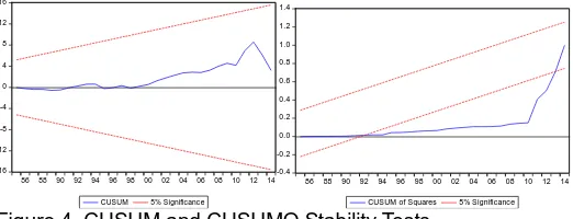
86 88 90 92 94 96 98 00 02 04 06 08 10 12 14 CUSUM of Squares 5% Significance Figure 4. CUSUM and CUSUMQ Stability Tests
Figure 4. shows the stability test through CUSUM and CUSUMQ estimates. This study refers to Bahamani and Harvey (2009), before the model estimation is carried out before the cumulative sum of recurvise residual test (CUSUM test) and the cumulative sum of square of the residual test (CUSUMQ test) stability test are performed. The results of the analysis show that the CUSUM test has been stable, while in the CUSUMQ test it looks slightly rejecting the stability of the model. Overall, both of the parameter analyzes, namely CUSUM and CUSUMQ have stated the stability of the model. Table 4. Results of the Engle-Granger Causality Test
Null Hypothesis: Obs F-Statistic Prob.
EC does not Granger Cause CO2 32 5.00740 0.0141
CO2 does not Granger Cause EC 0.03072 0.9698
FDI does not Granger Cause CO2 32 4.94820 0.0148 CO2 does not Granger Cause FDI 2.23941 0.1259
GDP does not Granger Cause CO2 32 6.77048 0.0041
CO2 does not Granger Cause GDP 0.49030 0.6178
FDI does not Granger Cause EC 32 0.76344 0.4759
EC does not Granger Cause FDI 2.44119 0.1060
GDP does not Granger Cause EC 32 0.03995 0.9609
EC does not Granger Cause GDP 0.04122 0.9597
GDP does not Granger Cause FDI 32 2.90350 0.0721
FDI does not Granger Cause GDP 0.41291 0.6658 From table 4. some conclusions can be drawn, including: a. The variable energy consumption (EC) statistically and significantly affects the variable carbon dioxide (CO2) emissions in Indonesia, this is evidenced by a probability value of 0.0141 which is smaller than alpha 0.05. While the variable carbon dioxide (CO2) emissions are statistically and not significantly affect vaiabel, this is evidenced by a probability value greater than alpha 0.05, which is equal to 0.9698. Based on the Engle-Granger causality test found a unidirectional relationship between energy consumption and carbon dioxide emissions;
b. FDI variables significantly affect the CO2 variable, this is evidenced by the probability value of 0.0148, whereas the opposite of CO2 does not significantly affect FDI because the probability value is greater than 0.05, which is 0.1259. Based on the Engle-Granger causality test it was found that there was a direct relationship between FDI and carbon dioxide emissions;
c. The GDP variable influences the CO2 variable in Indonesia significantly, this is indicated by the probability value of the GDP variable which is smaller than 0.05, which is equal to 0.0041. On the other hand the CO2 variable shows a non-significant effect on the GDP variable, this is based on the probability value of CO2 which is greater than 0.05, namely 0.6178. Based on the Engle-Granger causality test found a
unidirectional relationship between GDP and carbon dioxide emissions;
d. Based on the Engle-Granger causality test, no direct or two-way relationship was found between FDI and energy consumption; This is known from the probability value that is greater than the alpha value
e. Based on the Engle-Granger causality test, no directional or two-way relationship was found between GDP and energy consumption; This is known from the probability value that is greater than the alpha value
f. Based on the Engle-Granger causality test, no direct or two-way relationship was found between GDP and FDI. This is known from the probability value that is greater than the alpha value
Dynamic Ordinary Least Squares (DOLS) method is a method used to determine variable behavior in the short term that is influenced by the previous time lag. This method explains related to the influence of the independent variable on the dependent variable in the long run. DOLS is a development of the OLS method, where model estimation focuses on the influence of previous independent variables. Therefore in the Dynamic Ordinary Least Squares (DOLS) model the optimum lag selection is needed, this is done in order to obtain the best DOLS model. The lag selection is obtained from the lowest akaike information criteriation (AIC), Schawarz criteriation (SC) and Hannan quinn information criteriation (HQ) values. Meanwhile, the results of the analysis using the DOLS method in this study are illustrated in table 5. Based on the DOLS analysis there are similarities in the lags used in estimating each model. This is indicated by the minimum SC value in each lag tested. The SC value in each lag has the purpose of knowing the best DOLS model to be used in the study.
Table 5. Optimum Lag Test Results
Lag AIC SC HQ
1 0.618385 0.300944 0.511575
2 0.727912 0.269870 0.576084
3 0.696010 0.094661 0.499985
4 0.754648* 0.007343* 0.515579*
5 0.713700 0.182114 0.433142
6431 After going through the previous test stages, we can
estimate the Dynamic Ordinary Least Squares (DOLS) regression model. Where the stages that have been passed consist of root test - unit root (unit root test) and degree of integration, cointegration test and optimum lag test.
After knowing optimum lag in the DOLS model with lag 4, it is shown as follows:
Table 6. Results of Dynamic Ordinary Least Squares (DOLS) Regression Analysis.
Variable Coefficient Std. Error t-Statistic Probability EC -0.000727 0.001592 -0.456266 0.6547 FDI 0.008262 0.003289 2.512249 0.0239* GDP 2.82E-08 5.39E-08 0.523738 0.6081 EC(-1) 0.000332 0.001625 0.204318 0.8409 FDI(-1) 0.003537 0.004412 0.801756 0.4352 GDP(-1) -5.85E-08 7.06E-08 -0.828267 0.4205 EC(-2) 0.001790 0.001618 1.106694 0.2859 FDI(-2) -0.003868 0.003764 -1.027635 0.3204 GDP(-2) -3.47E-09 7.01E-08 -0.049535 0.9611 EC(-3) 0.001605 0.001654 0.970146 0.3474 FDI(-3) -0.006286 0.004146 -1.516132 0.1503 GDP(-3) 2.28E-09 7.31E-08 0.031212 0.9755 EC(-4) -0.001319 0.001307 -1.009409 0.3288 FDI(-4) 0.007305 0.004078 1.791059 0.0935 GDP(-4) 3.87E-08 5.64E-08 0.686293 0.5030 R-Squared 0.954918
*) Significant at α = 5%
The coefficient value in the estimation results illustrates how much the long-term relationship of the independent variable to the dependent is based on the Dynamic Ordinary Least Squares (DOLS) analysis method. Table 6. illustrates the estimation of the effect of the independent variable on the dependent variable using R-Squarred from the estimation of Dynamic Ordinary Least Squares (DOLS) in proving the influence of FDI, economic growth, and energy consumption on the variable carbon dioxide emissions. The estimation results show that the R-Squarred value is 0.954918, this indicates that there is an interplay between the independent variables and the dependent variable.
Based on Table 6. there is a dynamic change in carbon dioxide emissions, so that policy makers cannot provide certainty regarding the conditions of the upcoming CO2 emission policy. These results are in line with the changes in the global economy from time to time. Column 4 and column 5 in table 6. show the value of t-statistics and probabilities, where each variable shows significant and insignificant results on each lag. The estimation results are in accordance with the Environmental Kuznets Curves and Hypothesis Pollution theory in Indonesia in the context of sustainable economic development.
Table 7. Test of Classical Assumptions
Diagnosis Test Test Output Probability Description Multicollinearity Variance
Inflation Factors
1.060035 - Multicollinearity does not occur
Autocorrelation Durbin – Watson
- 1.345805 Autocorrelation does not occur Heterokesastici
ty
White 0.7799 0.8624 Heteroscedasticit y does not occur Normality
Jarque-Bera
4.554594 0.102561 Normal distribution
Linearity Ramsey-Reset
0.29599 0.7693 Linear data
Table 7. describes related to models in research that have met the classical assumptions. The classic assumption test results were calculated using multicollinearity diagnosis, autocorrelation, heterocedasticity, normality, and linearity. Based on the multicollinearity test that has been done shows that the Centered VIF values for both X1, X2 and X3 are 1.060035, 1.009674, and 1.06507 where the value is less than 10, it can be stated if there is no multicollinearity problem in the prediction model used .
The autocorrelation test aims to test whether in the linear regression model there is a correlation between the error in period t and the error in the previous period. Based on the autocorrelation test that has been done, the DW number is 1.345805 in the DW table for k = 4 and n = 34. While the lower limit value (dl) is 1.1426 and the upper limit (du) is 1.7386. If the value dl <d> du, then there is no autocorrelation.
Heterocedasticity test is carried out in order to test whether in the regression model there is a similarity of variance from residual values at the first observation to other observations. The assumption of heterocedasticity rejects at α = 5% and 10%. Heterocedasticity test in this study used white (cross term). Based on table 7. estimating the variable significance value above 0.05, which is equal to 0.7799, the results show no heterocedasticity. which states more than alpha 0.05.
The normality test is done with the aim of whether in a regression model, the independent variable, the dependent variable has normal distributed data or not. If in each variable has data that is normally distributed, the regression model is said to be good. In this study using the Jarque test - Bera to see the normality of the data on each variable. Is the probability value> significance level 5%, then the data distribution is said to be normal. Conversely, if the probability value is <5% significance level, then the data distribution is not normal. Table 7. illustrates the results of a probability of 0.102561, indicating that the model is normally distributed.
Linearity test is done in order to see the relationship between independent variables and dependent variables are linear or not. The criteria for conducting this test are if the probability value is significant > 5%, then the relationship between the independent variable and the dependent variable is linear. Table 7. illustrates the results of the linearity test that the variable has a probability value of 0.7693, it shows that the research variable is linear.
REFERENCES
[1] Arrow, K., dkk. 1995. Economic Growth, Carrying Capacity, and the Environment. Science. (268), 520-521.
[2] Grossman,G.M., dan Krueger,A.B.1991.Environmental impacts of the north American free trade agreement.
NBER Working paper (3914).
[3] Kizilkaya, Oktay. 2017. The Impact of Economic Growth and Foreign Direct Investment on CO2 Emissions: The Case of Turkey. Turkish economic review, Volume 4 March 2017 Issue 1.
[4] Kuznets, Simon. 1955. Economic Growth and Income Inequality, American Economic Review 45(1):1-28.
in Malaysia: DO foreign direct investment and trade matter? Energy Policy. (68): 490-497.
[6] Lee, J.W., 2013. The contribution of foreign direct investment to clean energy use, carbon emissions and economic growth, Energy Policy, vol. 55, p. 483-489.
[7] Linh, D dan Lin S. 2014. CO2 Emissions, Energy Consumption, Economic Growth and FDI in Vietnam.
[8] Omri, A. Nguyen, D. dan Rault, C. 2014. Causal Interactions Between CO2 Emissions, FDI, and Economic Growth: Evidence From Dynamic Simultaneous Equation Models. MPRA Paper (82504).
[9] Ozturk, Z dan Oz, D.2016. The Relationship between Energy Consumption, Income, Foreign Direct Investment, and CO2 Emissions: The Case of Turkey. Journal of The Faculty of Economics. Volume 6, Issue 2, pp. 269-288.
[10]Plummer, Micael. 2009. Global Economic Crisies and Its Implications For ASEAN Economic Coorporation. Policy studies No. 55.
[11]Ravenhill, J., 2014. Global Political Economy, 4th ed., Oxford, United Kingdom: Oxford University Press.
[12]Sadorsky, P., 2010. The impact of financial development on energy consumption in emerging economies, Energy Policy, (5) vol. 38, p. 2528 – 2535.
[13]Sbia, R., M. Shahbaz dan H. Hamdi, 2014. ―A contribution of foreign direct investment, clean energy, trade openness, carbon emissions and economic growth to energy demand in UAE‖, Economic Modelling, vol. 36, p. 191-197.