Efficient algorithms for fast integration on large data sets from multiple sources

R E S E A R C H A R T I C L E

Open Access

Efficient algorithms for fast integration on large

data sets from multiple sources

Tian Mi

, Sanguthevar Rajasekaran

and Robert Aseltine

Abstract

Background:Recent large scale deployments of health information technology have created opportunities for the integration of patient medical records with disparate public health, human service, and educational databases to provide comprehensive information related to health and development. Data integration techniques, which identify records belonging to the same individual that reside in multiple data sets, are essential to these efforts. Several algorithms have been proposed in the literatures that are adept in integrating records from two different datasets. Our algorithms are aimed at integrating multiple (in particular more than two) datasets efficiently.

Methods:Hierarchical clustering based solutions are used to integrate multiple (in particular more than two) datasets. Edit distance is used as the basic distance calculation, while distance calculation of common input errors is also studied. Several techniques have been applied to improve the algorithms in terms of both time and space: 1) Partial Construction of the Dendrogram (PCD) that ignores the level above the threshold; 2) Ignoring the

Dendrogram Structure (IDS); 3) Faster Computation of the Edit Distance (FCED) that predicts the distance with the threshold by upper bounds on edit distance; and 4) A pre-processing blocking phase that limits dynamic

computation within each block.

Results:We have experimentally validated our algorithms on large simulated as well as real data. Accuracy and completeness are defined stringently to show the performance of our algorithms. In addition, we employ a four-category analysis. Comparison with FEBRL shows the robustness of our approach.

Conclusions:In the experiments we conducted, the accuracy we observed exceeded 90% for the simulated data in most cases. 97.7% and 98.1% accuracy were achieved for the constant and proportional threshold, respectively, in a real dataset of 1,083,878 records.

Background

Increased use of electronic medical record systems and the development of health information exchanges have enormous potential to expand our understanding of the health of diverse patient populations. These efforts would be greatly augmented by the capacity to integrate patient medical records with disparate public health, human ser-vice, and educational databases, which usually do not have a universal identifier. For instance, health agencies may be interested in the integrated patients’ records across mul-tiple hospitals to track complete patients’health histories, to reveal mechanisms behind certain diseases, or to find reasons for local diseases. Data integration techniques for

identifying records belonging to the same individual that reside in multiple datasets, in the absence of any universal identifier,can improve health observation [1], improve in-jury surveillance systems, and health policy decisions [2] etc. It is also applied in health care insurance claims [3] and linkage of patients and health test results [4]. Data in-tegration is also used in other areas, such as similarity de-tection of digital files and document fingerprinting [5,6]. Typically, integration of datasets is done without the exist-ence of a global identifier [State of Connecticut. Connecti-cut Health Information Plan: A roadmap for improving access to health data. 2009 May. (unpublished report)]. Since errors might have been introduced while entering information, prediction of a record’s owner can never be 100%correct.

When there are only two data setsA andB, the data integration problem is to decide if the records aandb

* Correspondence:[email protected];[email protected] 1

Department of Computer Science and Engineering, University of Connecticut Storrs, Connecticut, USA

Full list of author information is available at the end of the article

belong to the same person (for every ða;bÞ 2ABÞ. Traditional approaches compare each record pair itera-tively and generate a comparison vector. As a result, each record pair is classified as a true match, possible match, or true non-match. Usually a learning algorithm is employed for this classification [7]. The data integra-tion problem that we are facing is much more challen-ging: 1) the records are from two or more sources; 2) the total number of records is quite large (a million or more) with very limited number of attributes to com-pare, and 3) the same dataset may have multiple records for individuals.

To apply the traditional method on multiple data sets may have some difficulties when dealing with the above challenges: 1) The cross-product of the datasets could be prohibitively large. For instance, consider ten datasets with two records in each. The number of 10-tuples is 210=1024. If we haveqdatasets consisting ofn1,n2,. . ., nq records, respectively, then the total number of

q-tuples to be enumerated is n1n2. . .;nq . There-fore, it is impractical to process large datasets. 2) One may want to ignore tuples and still process based on pairs. However this may lead to difficulties such as the pair(A, B)are decided to be matched while the pairs(A, C) and (B, C) being decided to be non-matched. 3) If tuples being used, redundant computation happens fre-quently when comparing records, for instance, recordsA and B may appear many times in different tuples and therefore in different tuples repeated computation on A and Bmay be done. And memory could be a bottleneck if we generate all possible tuples. Also, if pairs are used, the classification may suffer from poor accuracy. For ex-ample, a simplistic approach to matching three or more data sets involves matching two data sets iteratively, with the result of matching the first two data sets used as in-put for matching with the third data set, and so on. However, with this approach the final results are highly sensitive to the ordering of the datasets. Because of these disadvantages, the traditional probabilistic model seems to be inadequate for integrating multiple data sets.

Therefore, in this paper, we propose a new model to integrate multiple datasets. We employ hierarchical clus-tering [8] and avoid the computation of cross-products. Currently we use two methods to deal with common errors in the input data, typing distance and sound dis-tance. But other comparison methods can easily be added into our model. Besides, our algorithms also take care of the following types of errors: reversal of the first and last names, nickname usage, and attribute trunca-tion. Our algorithms are both time and space efficient. The excellent results from our experiments show that our clustering model is robust and promising when deal-ing with large data. With our model, new records can be easily inserted into old results without any

re-computations on the old data once the old data dendro-gram from Hierarchical Clustering is stored.

Methods

Previous approaches

Traditional approaches mainly involve two steps: com-parison of record pairs to generate comcom-parison vectors, and classification of record pairs into three sets of true match, possible match, and true non-match based on the comparison vectors [9,10]. A probabilistic model was introduced by Fellegi and Sunter in 1969 [11], in which comparison only considers match/non-match values. A lot of studies have been done following the probabilistic model [12-14]. Expectation maximization (EM) algo-rithm has been used to get better decision rules when maximum likelihood is reached in [15]. While a rela-tional probability model was used for citation matching [16], conditional models have been proposed to capture the dependency features under certain background, for instance, using conditional random fields in context [17,18]. Based on such conditional models, deduplication has been studied in relational databases of different data types, e.g. information of an entire record is kept in dif-ferent data tables [19,20]. This probabilistic model can also support categorical comparison values [14]. Several continuous-value comparisons also appear to deal with typographic errors [21], such as Hamming Distance, Edit Distance [22], Soundex Code and Metaphone (http:// www.sound-ex.com/alternative_zu_soundex), Jaro-Winkler Comparison [23], Q-grams (or N-grams) [24], Longest Common Substring [25], and so on.

parallel algorithms for it have also appeared (see e.g., [46-48]). Given a set of n points to be clustered, the ag-glomerative hierarchical clustering starts with n clusters where each cluster has a single input point with a dis-tance of 0. From there on, the algorithm proceeds in stages. In each stage the two closest clusters are merged into one and the distance of this new cluster is the dis-tance between the merged clusters. The stages of mer-ging happen until we are left with one cluster (containing all the input points). We can cut the tree at any desired threshold level. Note that each cluster is associated with a distance. All the root clusters at the threshold level will be output by the algorithm. Any hierarchical clustering algorithm can be classified based on the distance measure used. In this paper we use the single linkage clustering. It has been shown that results are similar using different linkage in Hierarchical Clus-tering [49], and single linkages has the advantage in time complexity [47].

Basic methodology

Our approach for data integration is to treat each record in each data set as a point in a multi-dimensional space. The dimension of this space is decided by the number of attributes in the records. We then define an appropriate distance measure for these points. Followed by this, we cluster these points and the clusters lead us to the iden-tification of common records.

Record distance calculation

In this paper, we consider attributes such as the first name, last name, gender, zip code, etc. However, the techniques described are generic and should be applic-able for any set of attributes. We define the distance be-tween two records in a number of ways by appropriately combining attribute distances. We use RD(R1,R2)to

de-note the distance between two recordsR1andR2. Given

R1andR2from any data sets, the common attributes of

the two records are used to calculateRD(R1,R2).

Definition 1: Assume that each of the two records R1

and R2from any data set have n common attributes and

let d1, d2,. . ., and dn be the attribute distances between

these records. Then, RD(R1,R2) is defined as d1+ d2+

. . .+ dn. Here di is the distance between the ith attribute

of R1 and the same attribute of R2. In this paper, the

combination operator we consider is addition for simpli-city, but other methods, like giving different weights to different attributes could be easily plugged in.

We consider two kinds of input errors, based on typing errors and sound similarity. We use the edit distance as the basic distance measure for the typing errors, while Metaphone is used to deal with errors based on sound similarity. The Edit Distance (also known as the Levensh-tein Distance) between two strings is the minimum

number of operations, such as deletion, insertion, and ex-change that are required to transform one string to the other [22]. One lower bound on the edit distance between two strings is the difference in the lengths of the two strings. One could use dynamic programming to compute the edit distance between two strings of lengthnand m, respectively, inO(mn)time (see e.g., [50]). With the Four-Russians speedup, which partitions the dynamic program-ming table into blocks and looks up the distance of each block from a pre-computed block offset function, the edit distance can be computed inO(l2/log(l))time when an ap-propriate block size is chosen (wherelis the length of the two strings) [51]. In this paper, we assume a penalty of1 for each of the operations insertion, deletion, and ex-change. Given two attributesA1andA2, the edit distance

of(A1,A2)is the attribute distance based on edit distance.

We incorporate into edit distance several methods to deal with common typing errors, such as 1) Reversal of the first name and the last name (reversal distance): In this case we use the smaller of the distance between the names and the distance between one name and the reversal of the other; 2) The use of nicknames (nickname distance): In this case we look up a nickname table (http://www.cc. kyoto-su.ac.jp/~trobb/nicklist.html) and use the smallest edit distance; and 3) Truncation of attributes (truncation distance): only consider the first few letters. Given two names, thename distancebetween them is defined as the smallest distance obtained from the names’edit distance, reversal distance, nickname distance, and truncation dis-tance. Errors based on pronunciation or sound similarity is another main issue when data is input. Metaphone is a phonetic algorithm to encode strings based on phonetic similarity, which works more effectively than the Soundex Coding. Phonetic distance between two attributes is defined as: 1) zero, if the Metaphone codes of them are the same; 2) edit distance of the Metaphone codes, otherwise.

The basic algorithm

We employ hierarchical clustering to deal with the prob-lem of integrating multiple (more than two) datasets. Our basic algorithm (Algorithm 1) is to take every rec-ord in each data set as a point (in an appropriate space). Single linkage hierarchical clustering is applied on these points. The clustering yields a dendrogram. A relevant threshold is employed to cut this dendrogram to obtain clusters of interest. In Step 2, a threshold is needed to collect the required clusters. We provide two types of thresholds - constant and proportional thresholds. The constant threshold allows a certain number of errors oc-curring in record comparisons, while the proportional threshold requires the number of errors to be limited to a percentage of the total record length.

Step 1. Construct the dendrogram using hierarchical clustering.

Step 2. Cut the dendrogram at the level of a threshold. Collect the root clusters at the threshold level and output.

Ideally, each cluster will only have points correspond-ing to the same person, i.e., all the versions of the same record will be in one cluster and this cluster will not have any other records. However in practice this may not always be the case. Thus we characterize the per-formance of this technique with an accuracy parameter (See RESULTS Section).

Iflis the maximum length of any record, the distance between two records can be computed in O(l2) time. Therefore, when the total number of records is n, Steps 1 and 2 needO(n2l2)time andO(n2)space.

Improved algorithms

Algorithm 1 takes too much time and space even on rea-sonably small data sizes. Note that the time and space requirements of Algorithm 1 are quadratic in the total number of records. Data sets of practical interest have millions of records. Table 1 displays the performance of Algorithm 1 on small datasets. Extrapolating from the numbers shown in this table, we can expect that Algo-rithm 1 will take around 20 hours when the number of records is100,000. To overcome the shortcomings of Al-gorithm 1, we have employed a series of techniques to improve its performance. In this section we describe these techniques.

Partial construction of the dendrogram

Instead of building the entire dendrogram and cutting at the threshold level, the idea here is to construct only portions of the tree that are below the threshold level. The resultant algorithm is shown as Algorithm 2.

Algorithm 2: PCD

Step 1. Collect all the records in all the data sets. Each such record is a cluster by itself at level 0 initially. Step 2. Calculate the record distances between each pair of clusters. Keep a nearest neighbor for each cluster.

Step 3. Find the pair of clusters with the smallest distance.

Step 4. If this distance is smaller than or equal to the threshold, then merge the two clusters into a new cluster with the distance as the new cluster’s level. Otherwise, go to Step 7.

Step 5. Update the pairwise distances and the new nearest neighbors’information.

Step 6. Repeat Steps 3, 4, and 5 until we end up with a single cluster.

Step 7. Collect and output the root clusters.

Although Algorithm 2 also takes O(n2l2) time, its expected run time is better than that of Algorithm 1. This is especially true if the error rate is low. If the errors in the records occur with a low probability, then the threshold value will be low and we only have to con-struct a small portion of the dendrogram.

Ignoring the dendrogram structure

Since only certain clusters are collected as the output, the structure of the dendrogram is not necessary. Algo-rithm 3 shows the details of this technique.

Algorithm 3: IDS

Step 1. Collect all the records in all the data sets. Let this collection beD.

Step 2.While Dis not emptydo

Pick one of the records in D arbitrarily. Let R be this record. We will form a cluster CR corresponding

toRas follows. To begin withCRhas onlyRin it. We

identify all the records inDthat are at a distance of≤ threshold from R. Let the collection of these records beC’. Add all the records ofC’toCR. Followed by this

identify all the records of D that are at a distance of

≤thresholdfrom any of the records ofC’. Let the col-lection of these records be C”. Add all the records of C’’ to CR. Continue this process of identifying

neigh-bors and adding them to CR until no new neighbors

can be found. At this point output CR. This is one of

the clusters of interest. SetD:=D - CR.

Since Algorithm 3 does not generate a distance matrix, its memory usage is only O(n) and the worst case run time is stillO(n2l2).

Faster computation of the edit distance

The general algorithm for edit distance computation takes quadratic time (see e.g., [22,50]). Since we have to calculate edit distances for a total ofn2times, a speedup in edit distance calculation will improve the run time on the entire data integration task. The four-Russians speedup algorithm on edit distance runs in O(l2/log(l)) time, when a block size is chosen to be (log3σ (l))/2

(where σ is the alphabet size and l is the length of two strings). However, unfortunately, it is inapplicable due to the short length of the strings involved since in this problem,σ=26and usuallyl≤50.

Observation 1: The edit distance between two strings is always larger than or equal to the difference in the lengths of the two strings.

It is easy to see that even if one stringS1is a substring

of the other S2, it still needs|S2|-|S1| number of inserts

bound can help to see whether the edit distance between two strings is larger than the threshold even before the calculation of the edit distance. In this case we can omit the calculation of the edit distance.

In summary, lettbe a given a threshold. If the distance between two stringsS1andS2is less than or equal tot, then

we can compute this distance in O tlð Þtime;wherel¼ min Sfj j1;j jS2g.

Dynamic programming is typically used to compute the distance between two strings. This algorithm employs a table of sizellðwherel¼max Sfj j1;j jS2gÞto

compute partial distances (see e.g., [34]). If the edit dis-tance between two strings is smaller than t, then the trace-back path of the dynamic programming table should be within a strip of size (2 t + 1) centered on the diagonal. The diagonal is where we align the ith charac-ter of one string to the same ith character of the other string. Departure from the diagonal means insertion or deletion, so when at most t inserts or deletions are allowed, the trace-back path is of departure at most t from the diagonal in a row. If the edit distance is smaller than t, what we calculate is the accurate edit distance. Otherwise, what we calculate is not accurate, but since we know that the edit distance is more than t, it does not matter that the edit distance computed is not accur-ate. We refer to this technique of computing edit distances as FCED (fast computation of edit distances).

This idea is also described in Gusfield's book ([52] 261– 262). In particular, in any row, column, or diagonal of the dynamic programming table (for edit distance com-putation), two adjacent cells can have values that differ by at most one ([52] 305–306). Also, in any diagonal of the dynamic programming matrix D (for edit distance computation), either D i½ ¼;j D i½ 1;j1;orD i½ ¼;j D i½ 1;j1 þ1. (MatrixDis defined as follows. If we are interested in computing the distance between two strings X ¼x1x2. . .xn;andY ¼y1y2. . .ym using dy-namic programming, then a matrix of size n×m will be employed. In particular, D[i,j] will be the distance be-tween x1x2. . .xi andy1y2. . .yj (for all values of i and j)). We can see that D i½ 6¼;j D i½ 1;j1 1 , then D i½ ;j is calculated from D i½ 1;jorD i½;j1. Without loss of generality, assume that D i½ ¼;j D i½ 1;j þ1: Then D i½ 1;j1 ¼D i½ ;j 2, which is a contradiction.

This fact implies that the values along the diagonal of the dynamic programming table are non-decreasing.

Using Observation 1, we first check if the edit distance is larger than the threshold. If not, we employ theO(tl)time algorithm as described above. We keep checking the diag-onal to see whether the allowed threshold t is broken through. If the edit distance is seen to be larger than the threshold, the algorithm terminates immediately. Other-wise, the accurate edit distance is calculated and returned. In this algorithm, the threshold is treated as the current Table 1 Experimental results on simulated data sets (constant threshold)

Algorithm Com Acc Time(ms) Com Acc Time(ms) Com Acc Time(ms)

BIA 99.4% 98.8% 14702 98.5% 97.0% 342411 - -

-PCD 99.4% 98.8% 12422 98.5% 97.0% 334583 - -

-RDED IDS 99.4% 98.8% 11562 98.5% 97.0% 291162 99.7% 99.3% 1200810

t = 30 IDS(FCED) 99.4% 98.8% 6031 98.5% 97.0% 164307 99.7% 99.3% 693665

TPA 92.2% 78.3% 406 90.7% 69.9% 7703 97.7% 91.8% 39843

TPA(FCED) 92.2% 78.3% 265 90.7% 69.9% 5266 97.7% 91.8% 21640

BIA 99.4% 98.8% 14453 98.3% 97.0% 354332 - -

-PCD 99.4% 98.8% 13812 98.3% 97.0% 360613 - -

-NDED IDS 99.4% 98.8% 13859 98.3% 97.0% 317052 99.6% 99.4% 1351910

t = 30 IDS(FCED) 99.4% 98.8% 9016 98.3% 97.0% 204071 99.6% 99.4% 861785

TPA 92.2% 78.3% 469 90.7% 70.0% 9484 97.7% 91.8% 42436

TPA (FCED) 92.2% 78.3% 359 90.7% 70.0% 6140 97.7% 91.8% 27155

BIA 98.8% 98.8% 11000 96.9% 96.4% 301960 - -

-PCD 98.8% 98.8% 11234 96.9% 96.4% 299756 - -

-PDED IDS 98.8% 98.8% 10547 96.9% 96.4% 254805 98.8% 98.9% 1046654

t = 30 IDS(FCED) 98.8% 98.8% 5390 96.9% 96.4% 145604 98.8% 98.9% 587013

TPA 92.4% 78.6% 391 90.7% 69.9% 7516 97.7% 91.8% 33499

TPA(FCED) 92.4% 78.6% 235 90.7% 69.9% 4313 97.7% 91.8% 20312

distance allowed. While dynamically calculating the edit distance, the diagonal value is compared with the threshold. If the value is already larger than the threshold, no further calculation is necessary and an infinite distance is given for such comparisons. If there is another pair of attributes to compare, a new distance allowed is computed as the threshold minus the distance already used. This method is implemented in Algorithm 3, and Algorithm 4 (in the next section).

A two-phase algorithm

Now we describe a two-phase algorithm. In the first phase (called a blocking phase), records sharing some-thing in common are indexed into the same block. Records in each block will be integrated later. Blocking phase uses the last nameattribute, which is considered more accurate than the first name.

In each record, the last name is parsed into l-mers (usually 3-mer or 4-mer), and this record is added into blocks which are indexed by these l-mers. For instance, in the case of l=3, ``Rueckl" is indexed into 4 blocks: ``rue", ``uec", ``eck", and ``ckl". The total number of possible blocks is 26l. Since one record may belong to multiple blocks, after integration on each block, a post-processing is done to merge clusters with duplicate records. Details are shown as Algorithm 4.

Algorithm 4: TPA

Step 1. Collect all the records in all the datasets. Put them into blocks based onl-mersof the last names. Step 2. Integrate records in each block using the algorithm IDS.

Step 3. Merge the clusters with the same records.

Assuming that there are b blocks, integrating each block takes O((n/b)2l2)time on an average. Over all the b blocks the expected run time isO(n2l2/b). Note thatb is typically a large number. For 3-mer blocking, b = 263= 17576and for4-merblockingb = 264= 456976.

In summary, we have proposed four algorithms for multiple-source integration, together with six distance calculations: edit distance to handle common typos, re-versal distance to handle the last and first names rere-versal errors, nickname distance to handle the distances with nicknames, truncation distance to handle the errors with abbreviations, phonetic distance to handle the similarity of sound, and name distance to capture all features of edit, reversal, nickname, and truncation distances on names. Without loss of generality, we validated our algo-rithms on simulated data by 1) reversal distance for the first or last names and edit distance for the other attri-butes (RDED); 2) name distance in the first and last names and edit distance in the other attributes (NDED)

where the truncation length is 5 for both the first and the last names; and 3) phonetic distance in the first and last names and edit distance in the other attributes (PDED). For real data, because of the limited common attributes (only first name, last name, and date of birth), EDname calculates the edit distances based on the first

and the last names, EDall considers all the three

attri-butes,PDnamecalculates the phonetic distances based on

the first and the last names, and PDED calculates the phonetic distances on the first and the last names and edit distance on date of birth.

Results

We have implemented our technique in Java and tested it on simulated data sets, as well as some real datasets. Additional file 1 details the generation of the simulated data sets. Also, the real data sets come from the Con-necticut Health Information Network (CHIN), which have a total of 1,083,878records (Please see Additional file 2 for details).

Results on simulated data

Since our algorithms collect all the records from all the input datasets, the number of input datasets is not im-portant. The performance of our algorithms depends only on the total number of records (from all the data-sets). Therefore, we generate a single input dataset for each test. Three datasets of size1,000,5,000, and10,000 respectively, are generated following [53] (Please see Additional file 1 for details). The computer we have used has aCPU of Intel(R) 2.83 GHz Core(TM)2 Quad Q9550, with a memory of4 GB.

learning method is pretty safe. From Table 1 and Table 2 (tests marked by”-”were terminated after waiting for 30 minutes), in general, most accuracies and completeness exceed 90% which indicates our approach’s capability in records matching. Especially algorithm TPA with FCED technique has a dramatic improvement in the run time, for instance, using RDED in 10,000 data size, IDS took 1201 s, and IDS(FCED) took694 s, while TPA only took 40 s and TPA(FCED) took 22 s, which is roughly 30 times faster, though with some drop in the accuracy (e.g. 99.7%of IDS(FCED) to 97.7%TPA(FCED) in complete-ness and 99.3% to 91.8% in accuracy) due to the fact that in the blocking phase not all the records which per-tain to the same person can be indexed into the same block. This small drop in the accuracy may be worth-while, especially when dealing with large data and if time is a critical factor. As a result, we have employed TPA and TPA (FCED) on real data sets.

To validate the thresholds chosen in training, a 5-fold cross validation was used: partition the 10,000 records into 5 equal sets and randomly pick four sets as the training data to get the thresholds and the remaining as the testing data, and repeat 5 times. Table 3 shows the result of the 5-fold cross validation. Accuracies obtained (around ~98%) suggest that the thresholds identified in training are able to capture the general features of the data and therefore separate records of the same person from the others pretty well.

We also tested on a large dataset with 1,000,000 records. Results in Table 4 show the efficiency and ro-bustness of the proposed algorithms.

Results on real data

We have a total of 1,083,878 records and multiple records from one person in each of the four databases are common (Please see Additional file 2 for detail). A linkage gold- standard has shown that the attribute bination of Social Security Number, phonetically com-pressed first name, birth month, and gender is the best one to find record linkage [54]. However, the common attributes across all the 4 data sets were very limited: first name, last name, and date of birth, which increased the challenge to do the integration. EDname calculates

the edit distances based on the first and the last names, EDallconsiders all the three attributes,PDnamecalculates

the phonetic distances based on the first and the last names, and PDED calculates the phonetic distances on the first and the last names and edit distance on date of birth. The thresholds are obtained from training 4,000

Table 3 Accuracies in 5-fold cross validation on picking up the threshold

model1 model2 model3 model4 model5

constant = 30 99.3% 99.3% 99.7% 99.6% 97.3%

proportion = 0.35 99.2% 99.1% 99.4% 99.0% 97.0%

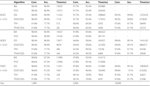
Table 2 Experimental results on simulated data sets (proportional threshold)

Algorithm Com. Acc. Time(ms) Com. Acc. Time(ms) Com. Acc. Time(ms)

BIA 98.4% 96.9% 14593 97.7% 95.4% 345880 - -

-PCD 98.4% 96.9% 13515 97.7% 95.4% 345645 - -

-RDED IDS 98.4% 96.9% 11422 97.7% 95.4% 298069 99.5% 99.0% 1225476

t = 0.35 IDS(FCED) 98.4% 96.9% 7125 97.7% 95.4% 173932 99.5% 99.0% 673650

TPA 91.8% 77.7% 515 90.4% 69.5% 9203 97.6% 91.7% 38499

TPA(FCED) 91.8% 77.7% 281 90.4% 69.5% 4500 97.6% 91.7% 23374

BIA 98.4% 96.9% 14547 97.8% 95.6% 384222 - -

-PCD 98.4% 96.9% 14156 97.8% 95.6% 381191 - -

-NDED IDS 98.4% 96.9% 13671 44.6% 99.6% 343927 99.6% 99.1% 1416142

t = 0.35 IDS(FCED) 98.4% 96.9% 9078 44.6% 99.6% 222305 99.6% 99.1% 884472

TPA 91.8% 77.7% 485 42.5% 90.5% 10140 97.6% 91.7% 45436

TPA(FCED) 91.8% 77.7% 344 42.5% 90.5% 6484 97.6% 91.7% 29030

BIA 98.6% 97.2% 11890 97.8% 95.5% 314115 - -

-PCD 98.6% 97.2% 12046 97.8% 95.5% 313006 - -

-PDED IDS 98.6% 97.2% 11031 97.8% 96.0% 272085 99.6% 99.1% 1083059

t = 0.35 IDS(FCED) 98.6% 97.2% 5937 97.8% 96.0% 165495 99.6% 9.1% 610262

TPA 91.8% 77.7% 250 90.1% 70.0% 7843 97.6% 91.7% 32827

TPA(FCED) 91.8% 77.7% 171 90.1% 70.0% 4297 97.6% 91.7% 21046

records, 1,000 from each database. The detailed results are shown in Table 4. Accuracy is estimated by the com-bination of Social Security Number and the internally assigned DDS identification number. Out of the total 1,083,878 records,896,174 records have valid identifiers so the analysis is based on the 896,174 records. While looking into the details of the results of EDname, we

found that most of the inaccurate clusters resulted when tautonyms exist, i.e., when there were records with exactly the same first and last names pertaining to differ-ent persons. 97.8% accuracy was achieved immediately when edit distance was used on all the three attributes for the constant threshold (98.1% for the proportional threshold) within around 30 minutes (1 hour), and 98.4% accuracy was received for PDED (98.1% for the proportional threshold) around 1 hour, where complete-ness is above 90% when all the three attributes were used, as shown in Table 4. In particular, the algorithm TPA (FCED) was about four to six times as fast as the algorithm TPA using edit distance, and even with edit distance of one attribute TPA (FCED) still speeds up about two times (PDEDin Table 4). The notion of nega-tive data is unclear to this multiple data integration problem and hence sensitivity and specificity analysis cannot be done. However, we perform a similar analysis to look further into our results. A four-category analysis is proposed. Any cluster of records is categorized into four: 1) (Type I), if a cluster contains only one person's records and contains all of this person's records; 2) (Type II), if a cluster contains only one person's records but not all of this person's records; 3) (Type III), if a cluster contains all the records of one person but also contains some other person's records; 4) other cases can be seen as errors (Type IV). Table 5 shows the results of this analysis. Type II clusters are nothing but incomplete clusters which still play a valuable role to people. Type III clusters are similar but a little less important. There-fore, only Type IV clusters are “true incorrect”. When using all the three attributes, this“true incorrect rate”is limited within about0.6%.

Comparison with the probabilistic model using FEBRL

FEBRL [26-28] is excellent for data linkage, which exploits most of the current techniques of indexing/ blocking, comparison, and classification.

Linkage of two datasets is compared in Table 6. Since any of the distance calculations of the proposed ap-proach considers certain common errors, like insertion, deletion, and so, to be fair, we chose to use a similar dis-tance calculation, the edit disdis-tance, in FEBRL, and we chose “FellegiSunter” from the classification methods as the probabilistic model to compare. From the real data, we randomly picked 1,000 vs. 1,000,2,000 vs. 2,000, and 3,000 vs. 3,000data sets as three groups of linkage tests. We usedIDS (FCED)as the non-blocking algorithm and TPA (FCED)as a blocking algorithm in the comparison. For each algorithm, we used EDname, EDall, and NDED

as the distance calculation. In FEBRL [26-28], only the best result was selected for a non-blocking algorithm and a blocking algorithm. It was found that the best results could be reached with 0.5 as the edit distance thresholds, respectively, and 0.3 and 0.8 as lower and upper threshold for “FellegiSunter”, and with blocking the fastest index method can be “CanopyIndex” with canopy method “Jaccard” and global tight and loose thresholds of0.8and 0.3and 3as the length of q-grams. Table 6 shows that the two approaches have similar Table 4 Experimental results on real data sets (N = 1,083,878)

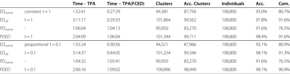
Time - TPA Time–TPA(FCED) Clusters Acc. Clusters Individuals Acc. Com.

EDname constant t = 1 1:52:41 0:27:29 94,381 87,756 108,800 93.0% 80.7%

EDall t = 1 3:11:17 0:29:33 101,864 99,562 108,800 97.8% 91.6%

PDname - 1:06:04 1:04:13 90,950 83,270 108,800 91.6% 76.5%

PDED t = 1 2:04:09 1:06:04 101,344 99,711 108,800 98.4% 91.6%

EDname proportional t = 0.1 1:55:24 0:30:56 94,521 87,966 108,800 93.1% 80.9%

EDall t = 0.1 3:14:37 0:44:05 101,254 99,346 108,800 98.1% 91.3%

PDname - 1:04:32 1:05:41 90,950 83,270 108,800 91.6% 76.5%

PDED t = 0.1 2:06:16 1:09:02 100,896 98,949 108,800 98.1% 90.9%

Table 5 Four-category analysis on real data sets (N = 1,083,878)

Type I Type II Type III Type IV

EDname constant t = 1 93.0% 2.2% 0.0% 4.8%

EDall t = 1 97.7% 2.1% 0.0% 0.2%

PDname - 91.6% 1.7% 0.0% 6.7%

PDED t = 1 98.4% 1.3% 0.0% 0.3%

EDname proportional t = 0.1 93.1% 2.2% 0.0% 4.7%

EDall t = 0.1 98.1% 0.1% 0.0% 0.4%

PDname - 91.6% 1.7% 0.0% 6.7%

accuracies. However, our approach takes less time for both non-blocking and blocking algorithms demonstrat-ing the robustness of our algorithms in handldemonstrat-ing large input datasets. For FEBRL with no blocking on 3000 vs. 3000, we terminated the program after waiting for 15 minutes with no response, since all the other methods can finish within around 20 seconds.

Discussion

To achieve a good accuracy, a good threshold value to cut the dendrogram of the hierarchical clustering is needed.

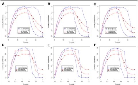
We show the relationship betweenAccuracy/Completeness and thresholds in Figure 1. A decent threshold is needed to get a nice accuracy or completeness, which depends on many parameters such as attributes compared, attribute distances applied, combination operation used, and even the specific data sets, and should be decided empirically. In this paper we provide some guidelines for picking an ap-propriate threshold value.

Using a training phase is always a good method to learn the threshold. We can think of the entire process of data in-tegration as consisting of two main processes. The first

Figure 1Relationship between thresholds and accuracy/completeness. (A)EDnamewith constant thresholds;(B)RDEDwith constant

thresholds;(C)NDEDwith constant thresholds;(D)EDnamewith proportional thresholds;(E)RDEDwith proportional thresholds;(F)NDEDwith

proportional thresholds.

Table 6 Performance comparison with FEBRL

Acc. Time(ms) Acc. Time(ms) Acc. Time(ms) Comments

100.0% 766 100.0% 3766 100.0% 8735 DSI(FCED) + EDname

99.0% 2125 100.0% 11171 100.0% 15922 DSI(FCED) + EDall

Our 99.0% 2563 98.2% 9172 97.7% 20391 DSI (FCED) + NDED

Algorithms 100.0% 187 100.0% 250 100.0% 469 TPA(FCED) + EDname

100.0% 234 100.0% 453 100.0% 828 TPA(FCED) + EDall

99.2% 203 98.4% 516 98.0% 1047 TPA (FCED) + NDED

FEBRL 100.0% 40438 100.0% 173597 - _>15 min no blocking

100.0% 1284 100.0% 2284 100.0% 3265 s With blocking

process is the training phase wherein we will be given records with identifiers to indicate which of them belong to the same person. In this phase we learn the values of all the underlying parameters (threshold, in particular). Once we learn the values of the parameters, in the second phase we can work on any (unknown) collection of datasets and inte-grate them. If the dataset given in the training phase is truly representative of the real world data, then the accuracy in the second phase will be high. This is typically true for any learning technique. The learning technique can only be as good as the training dataset. For example, in our experi-ments, for the simulated data test, the threshold was learned from datasets of size1,000(Table 1 and Table 2), and for real data test, the threshold was learned from 4,000 records, 1,000from each of the four data sets. Both of these training phases resulted in good results. Another way is to use the knowledge about the input datasets to get a threshold empir-ically. Generally speaking, the real world data may not have too many errors and a small threshold is always suggested. In our real data experiment, one million records are more than enough to suggest that the constant threshold of1and the proportional threshold of0.1would be promising.

Also, one may want to run the application multiple times with different thresholds. With the nature of Hier-archical Clustering, it is not necessary to re-calculate everything. If the whole dendrogram is kept, different thresholds are just different levels to cut the tree struc-ture and the result can be immediately output. Although a lot of studies have been made in record linkage, work has seldom been done on multiple data sets as relatively large as we discussed here. Merge/Purge is capable to handle millions of records in the parallel implementation [31]. Also, this is done by its simple clustering method of two phases, of which the first phase clusters data on an n-attribute key and the second phase applies the sorted-neighbourhood method within each cluster. Then further processes and decisions are made. Such simple clustering method supports the capability of Merge/ Purge to handle large data sets fast. Though at very low possibilities coincident of errors in these n-attribute keys may risk the general accuracy, it does not harm the good tradeoff between time and accuracy in Merge/Purge since it may happen at very small probabilities. We use distance calculations to plug in the hierarchical cluster-ing method, in the expectation that different calculation methods can be easily added into our approach and per-formance can be improved by new excellent calculation methods. And the efficiency is obtained by algorithm improvement within hierarchical clustering and the dis-tance calculation.

Conclusions

The ability to integrate diverse medical and public health datasets, particularly in this time of burgeoning availability

of data from health information exchanges, offers unprece-dented opportunities for health research and surveillance. A prerequisite for this, however, are techniques that allow for the simultaneous integration of multiple datasets that lack a shared numeric identifier. In this paper, we have pre-sented an approach for the integration of records from multiple datasets. We improved our basic idea based on several different methods and implemented and experimen-tally validated our approach. In addition to the standard at-tribute distance measures, we have also introduced attribute distances based on prior knowledge of commonly occurring mistakes. Hierarchical clustering is the basis of our approach. The accuracy we have obtained is very good indicating that our approach is promising.

Additional files

Additional file 1:Detailed generation of the simulated data [53].

Additional file 2:Introduction to the real data.

Competing interests

All authors declare that they have no competing interests.

Authors_’contributions

TM contributed to the implementation of the algorithms, testing and analysis on the synthetic and real data, manuscript preparation, algorithms development, and performance analysis. SR contributed to algorithms development, analysis of the results, performance analysis, and manuscript preparation. RA contributed to data preparation, results analysis, and performance analysis. All authors read and approved the final manuscript.

Acknowledgements

This research has been supported in part by the NSF Grants 0326155 and 0829916 and the NIH Grant R01-LM010101, and the State of Connecticut. We also want to thank Laurel Buchanan for the description of the real data in Additional file 2.

Author details

1_{Department of Computer Science and Engineering, University of}

Connecticut Storrs, Connecticut, USA.2_{Institute for Public Health Research,} University of Connecticut, East Hartford, Connecticut, USA.

Received: 24 October 2011 Accepted: 28 June 2012 Published: 28 June 2012

References

1. Fayyad U, Piatetsky-shapiro G, Smyth P:From data mining to knowledge discovery in databases.AI Mag1996,17:37–54.

2. Clark DE:Practical introduction to record linkage for injury research.Inj Prev2004,10(3):186–191.

3. Victor TW, Mera R:Record linkage of health care insurance claims.J Am Med Inform Assoc2001,8:281–288.

4. Maizlish N, Herrera L:A record linkage protocol for a diabetes registry at ethnically diverse community health centers.J Am Med Inform Assoc2005,

12:331–337.

5. Brin S, Davis J, Garcia-Molina H:Copy Detection Mechanisms for Digital Documents. InProceedings of the ACM SIGMOD Annual Conference: 22–25 May 1995; San Jose, CA. Edited by Carey Michael J, Schneider Donovan A. New York: ACM; 1995:398–409.

7. Gu L, Baxter R, Vickers D, Rainsford C:Record linkage: current practice and future directions.CSIRO Mathematical and Information Sciences Tech Rep

2003,3(3):83.

8. Zhao Y, Karypis G:Evaluation of hierarchical clustering algorithms for document datasets. InProceedings of the 11th international conference on Information and knowledge management: 4–9 November 2002; McLean, VA. New York: ACM; 2002:515–524.

9. Christen P, Goiser K:Quality and complexity measures for data linkage and deduplication. InQuality Measures in Data Mining. Volume 43. Edited by Guillet F, Hamilton H. New York: Springer; 2007:127–151.

10. Winkler WE:Overview of Record Linkage and Current Research Directions. [http://www.census.gov/srd/papers/pdf/rrs2006-02.pdf] 11. Fellegi IP, Sunter AB:A theory for record linkage.J Am Stat Assoc1969,64

(328):1183–1210.

12. Elmagarmid AK, Ipeirotis PG, Verykios VS:Duplicate Record Detection: A Survey.IEEE Trans Knowl Data Eng2007,19:1–16.

13. Winkler WE:Matching and record linkage. InBusiness Survey Methods. Edited by Brenda G, Cox, David A, Binder B, Nanjamma Chinnappa, Anders Christianson, Michael J, Colledge, Phillip S, Kott. New York: Wiley; 1995:355– 384.

14. Winkler WE:The State of Record Linkage and Current Research Problems. [http://www.census.gov/srd/papers/pdf/rr99-04.pdf]

15. Winkler WE:Improved Decision Rules In The Fellegi-Sunter Model Of Record Linkage. InProceedings of on Survey Research Methods, American Statistical Association. Volume 1. Alexandria, VA: American Statistical Association; 1993:274–279.

16. Pasula H, Marthi B, Milch B, Russell S, Shpitser I:Identity uncertainty and citation matching. InProceedings of the 2002 Conference on Advances in Neural Information Processing Systems: 9–14 December 2002; Vancouver, Canada. Edited by Becker S, Thrun S, Obermayer K. Cambridge, MA: MIT Press; 2003:1401–1408.

17. McCallum A, Wellner B:Conditional models of identity uncertainty with application to noun coreference. InProceedings of the 2004 Conference on Advances in Neural Information Processing Systems: 13–18 December 2004; Vancouver, Canada. Edited by Saul L, Weiss Y, Bottou L. Cambridge, MA: MIT Press; 2005:905–912.

18. Lafferty J, McCallum A, Pereira F:Conditional random fields: Probabilistic models for segmenting and labeling sequence data. InProceedings of 18th International Conference on Machine Learning: June 28-July 1 2001; Williamstown, MA. Edited by Brodley CE, Danyluk AP, Waltham MA. Waltham, MA: Morgan Kaufmann; 2001:282–289.

19. Culotta A, McCallum A:Joint deduplication of multiple record types in relational data. InProceedings of the 14th ACM international conference on Information and knowledge management: October 31-November 15 2005; Bremen, Germany. Edited by Herzog O, Schek HJ, Fuhr N, Chowdhury A, Teiken W. New York: ACM; 2005:257–258.

20. Parag, Domingos P:Multi-relational record linkage. InProceedings of the Tenth International Conference on Knowledge Discovery and Data Mining: August 22–25 2004; Seattle. Edited by Kim W, Kohavi R, Gehrke J, DuMouchel W. New York: ACM; 2004:31–48.

21. Christen P:A comparison of personal name matching: Techniques and practical issues. InProceedings of the Second International Workshop on Mining Complex Data: December 18–22 2006. Hong Kong. Los Alamitos (CA): IEEE Computer Society Press; 2006:290–294.

22. Levenshtein VI:Binary codes capable of correcting deletions, insertions, and reversals.Soviet Phys, Doklady1966,10(8):707–710.

23. Jaro MA:Advances in Record Linkage Methodology as Applied to Matching the 1985 Census of Tampa, Florida.J Am Stat Assoc1989,84(406):414–420. 24. Kukich K:Techniques for automatically correcting words in text.ACM

Comput Surv1992,24(4):377–439.

25. Friedman C, Sideli R:Tolerating spelling errors during patient validation.

Compu Biomed Res1992,25:486–509.

26. Christen P, Churches T, Hegland M:Febrl - a parallel open source data linkage system.Lect Notes Comput Sc2004,3056:638–647.

27. Christen P: InProceedings of the 14th International Conference on Knowledge Discovery and Data Mining: 24–27 August 2008; Las Vegas. Edited by Ying L, Bing L, Sunita S. New York: ACM; 2008:1065–1068.

28. Christen P:Febrl - a freely available record linkage system with a graphical user interface. InProceedings of the second Australasian workshop on Health data and knowledge management: 1–1 January 2008; Wollongong, Australia. Edited by Warren JR, Yu P, Yearwood J, Patrick JD, Warren JR, Yu P,

Yearwood J, Patrick JD. Darlinghurst (Australia): Australian Computer Society, Inc; 2008:17–25.

29. Elfekey M, Vassilios V, Elmagarmid A:Agrawal R, Dittrich KR, Ngu AHH. In

Proceedings of the 18th International Conference on Data Engineering: 26 February-1 March 2002; San Jose. Edited by Agrawal R, Dittrich KR, Ngu AHH. Los Alamitos (CA): IEEE Computer Society Press; 2002:17–28.

30. Lee ML, Ling TW, Low WL:Intelliclean: A knowledge-based intelligent data cleanser. InProceedings of the Sixth International Conference on Knowledge Discovery and Data Mining: 20–23 August 2000. Boston. New York: ACM; 2000:290–294.

31. Hernandez MA, Stolfo SJ:The Merge/Purge Problem for Large Databases. InProceedings of the 1995 ACM SIGMOD International Conference on Management of Data: 22–25 May 1995; San Jose. Edited by Carey MJ, Schneider DA. New York: ACM; 1995:127–138.

32. Hernandez MA, Stolfo SJ:Real World Data is Dirty: Data Cleansing and the Merge/Purge Problem.Data Min Knowl Disc1998,2(1):9–37.

33. McCallum A, Nigam K, Ungar LH:Efficient clustering of high-dimensional data sets with application to reference matching. InProceedings of the Sixth International Conference on Knowledge Discovery and Data Mining: 20– 23 August 2000. Boston. New York: ACM; 2000:169–178.

34. Wong W, Liu W, Bennamoun M:Tree-Traversing Ant Algorithm for Term Clustering based on Featureless Similarities.Data Min Knowl Disc2007,15

(3):349–381.

35. Ng RT, Han J:Efficient and effective clustering methods for spatial data mining. InProceedings of the 20th International Conference on Very Large Data Bases: 12–15 September 1994; Santiago de Chile, Chile. Edited by Bocca JB, Jarke M, Zaniolo C. San Francisco: Morgan Kaufmann Publishers Inc; 1994:144–155.

36. Vinh NX, Epps J, Bailey J:Information Theoretic Measures for Clusterings Comparison: Is a Correction for Chance Necessary?InProceedings of the 26th International Conference On Machine Learning: 14-18 June 2009; Montreal, Quebec, Canada. Edited by Danyluk AP, Bottou L, Littman ML. New York: ACM; 2009:1073–1080.

37. Clatworthy J, Buick D, Hankins M, Weinman J, Horne R:The use and reporting of cluster analysis in health psychology: A review.Br J Health Psychol2005,10(3):329–358.

38. Heyer LJ, Kruglyak S, Yooseph S:Exploring Expression Data: Identification and Analysis of Coexpressed Genes.Genome Res1999,9(11):1106–1115. 39. Hawse JR, Hejtmancik JF, Huang Q, Sheets NL, Hosack DA, Lempicki RA,et

al:Identification and functional clustering of global gene expression differences between human age-related cataract and clear lenses.Mol Vis2003,9:515–537.

40. Huang DW, Sherman BT, Lempicki RA:Systematic and integrative analysis of large gene lists using DAVID Bioinformatics Resources.Nature Protoc

2009,4(1):44–57.

41. Dennis G Jr, Sherman BT, Hosack DA, Yang J, Gao W, Lane HC,et al:DAVID: Database for Annotation, Visualization, and Integrated Discovery.

Genome Biol2003,4(5):3.

42. Sibson R:SLINK: An optimally efficient algorithm for the single-link cluster method.Computer J1973,16:30–34.

43. Day WH, Edelsbrunner H:Efficient algorithms for agglomerative hierarchical clustering methods.J Classification1984,1:7–24. 44. Murtagh F:A Survey of Recent Advances in Hierarchical Clustering

Algorithms.Computer J1983,26(4):354–359.

45. Kotsiantis SB, Pintelas PE:Recent advances in clustering: A brief survey.

WSEAS Trans Inf Sci Appl2004,1:73–81.

46. Li X:Parallel algorithms for hierarchical clustering and cluster validity.

IEEE Trans Pattern Anal Mach Intell1990,12(11):1088–1092.

47. Olson CF:Parallel algorithms for hierarchical clustering.Parallel Comput

1995,21(8):1313–1325.

48. Rajasekaran S:Efficient parallel hierarchical clustering algorithms.IEEE Trans Parallel Distrib Syst2005,16(6):497–502.

49. Mi T, Aseltine R, Rajasekaran S:Data Integration on Multiple Data Sets. In

Proceedings of the 2008 IEEE International Conference on Bioinformatics and Biomedicine: 3–5 November 2008; Philadephia. Edited by Chen X, Hu X, Kim S. Los Alamitos (CA): IEEE Computer Society Press; 2008:443–446.

50. Horowitz E, Sahni S, Rajasekaran S:Chapter 5, Dynamic Programming. In

Computer Algorithms. 2nd edition. Summit (NJ): Silicon Press; 2008:284–286. 51. Arlazarov L, Dinic EA, Kronrod MA, Faradzev IA:On economic construction of the transitive closure of a directed graph.Soviet Math, Doklady1970,

52. Gusfield D:Algorithms on strings, trees, and sequences: computer science and computational biology. Cambridge (England): Cambridge Univ. Press; 2007. 53. Christen P, Pudjijono A:Accurate Synthetic Generation of Realistic

Personal Information. InProceedings of the 13th Pacific-Asia Conference on Advances in Knowledge Discovery and Data Mining: 27–30 April 2009; Bangkok, Thailand. Edited by Theeramunkong T, Kijsirikul B, Cercone N, Ho TB. Berlin Heidelberg: Springer; 2009:507–514.

54. Grannis S, Overhage JM, McDonald C:Analysis of identifier performance using a deterministic linkage algorithm. InProceedings of the Annual Symposium of the American Medical Informatics Association: 9–13 November 2002; San Antonio, TX. Edited by Kohane IS. Philadelphia: Hanley & Belfus, Inc; 2002:305–309.

doi:10.1186/1472-6947-12-59

Cite this article as:Miet al.:Efficient algorithms for fast integration on large data sets from multiple sources.BMC Medical Informatics and Decision Making201212:59.

Submit your next manuscript to BioMed Central and take full advantage of:

• Convenient online submission

• Thorough peer review

• No space constraints or color figure charges

• Immediate publication on acceptance

• Inclusion in PubMed, CAS, Scopus and Google Scholar

• Research which is freely available for redistribution