R E S E A R C H A R T I C L E
Open Access
Data mining EEG signals in depression for
their diagnostic value
Mahdi Mohammadi
1, Fadwa Al-Azab
1, Bijan Raahemi
1, Gregory Richards
1, Natalia Jaworska
2, Dylan Smith
3,
Sara de la Salle
4, Pierre Blier
5and Verner Knott
5*Abstract
Background:Quantitative electroencephalogram (EEG) is one neuroimaging technique that has been shown to
differentiate patients with major depressive disorder (MDD) and non-depressed healthy volunteers (HV) at the group-level, but its diagnostic potential for detecting differences at the individual level has yet to be realized. Quantitative EEGs produce complex data sets derived from digitally analyzed electrical activity at different frequency bands, at multiple electrode locations, and under different vigilance (eyes open vs. closed) states, resulting in potential feature patterns which may be diagnostically useful, but detectable only with advanced mathematical models.
Methods:This paper uses a data mining methodology for classifying EEGs of 53 MDD patients and 43 HVs. This included: (a) pre-processing the data, including cleaning and normalization, applying Linear Discriminant Analysis (LDA) to map the features into a new feature space; and applying Genetic Algorithm (GA) to identify the most significant features; (b) building predictive models using the Decision Tree (DT) algorithm to discover rules and hidden patterns based on the reduced and mapped features; and (c) evaluating the models based on the accuracy and false positive values on the EEG data of MDD and HV participants. Two categories of experiments were performed. The first experiment analyzed each frequency band individually, while the second experiment analyzed the bands together.
Results:Application of LDA and GA markedly reduced the total number of utilized features by≥50 % and, with all frequency bands analyzed together, the model showed average classification accuracy (MDD vs. HV) of 80 %. The best results from model testing with additional test EEG recordings from 9 MDD patients and 35 HV individuals demonstrated an accuracy of 80 % and showed an average sensitivity of 70 %, a specificity of 76 %, and a positive (PPV) and negative predictive value (NPV) of 74 and 75 %, respectively.
Conclusions:These initial findings suggest that the proposed automated EEG analytical approach could be a useful adjunctive diagnostic approach in clinical practice.
Keywords:Depression, EEG, Genetic algorithm, Linear discriminant analysis, Decision tree, Sensitivity, Specificity
Background
Depression, a common psychiatric disorder with a life-time prevalence of ~ 20 % in the general population, is associated with high rates of disability, impaired psycho-social functioning and decreased life satisfaction [1]. Early recognition and accurate diagnosis of depression
are essential criteria for optimizing treatment selection and improving outcomes, thus reducing the economic and psychosocial burdens resulting from hospitalization, lost work productivity and suicide [2–4]. Guided by established classification criteria (DSM-5) [5], the diag-nosis of psychiatric disorders including depression relies solely on inferences based on self-reported information and observed behaviour. Identifying people with estab-lished depression does not usually present as a clinical challenge with standard clinical instruments but the potential for ambiguity, bias and low reliability of a
* Correspondence:[email protected]
5Institute of Mental Health Research at the Royal Ottawa Mental Health Care Centre, University of Ottawa, 1145 Carling Avenue, Ottawa, ON K1Z 7 K4, Canada
Full list of author information is available at the end of the article
even race [6].
Defined as objective biological measures indicating the state of a normal biologic process, pathogenic process, or pharmacological response to a therapeutic interven-tion [7], biomarker use for diagnostics has become stand-ard in day-to-day practice in medicine (e.g. cstand-ardiology, oncology) but there are no accepted biomarkers for MDD or other psychiatric disorders. Recent progress has pro-vided evidence that psychiatric disorders are brain dis-orders characterized by abnormalities in the structure, function and neurochemistry in distributed neural net-works [8]. Neuroimaging, which allows forin vivo access to these brain circuits, has increased our understanding of the pathophysiology of these disorders [9, 10] and is a leading candidate for the development of clinical bio-markers with potential use for diagnosis, prognosis and treatment of depression [11–16].
For biomarkers to be diagnostically useful, they need to be reliable and reproducible, providing sufficiently high levels of sensitivity and specificity in the detection and correct classification of distinct disorders [17]. Fur-thermore, for routine use in clinical practice, they should be inexpensive, noninvasive and easily accessible [17]. Compared to some other proposed brain imaging bio-markers derived from functional magnetic resonance imaging (fMRI), positron emission tomography (PET), and magnetic resonance spectroscopy (MRS), quantita-tive measurement of brain electrical signals taken from the scalp-recorded electroencephalogram (EEG) is a neu-roimaging technique with clear practical advantages as it does not involve invasive procedures, is widely available, easy to administer, well tolerated, and has a relatively low cost [18]. In addition to its growing potential as a bio-marker in the therapeutic drug development process [19, 20] and in predicting antidepressant treatment re-sponse [21–25], power spectral measures of resting state EEG oscillatory activity in different frequency bands (delta [<4 Hz], theta [~4–8 Hz], alpha [~8–12 Hz], beta [~12–30 Hz) have been shown to distinguish be-tween depressed patients and healthy controls [26- 28]. However, EEG biomarkers/biosignatures characterizing brain abnormalities in depressed patients tend to be limited to group-level comparisons. Although they are informative in elucidating the neuropathophysiology of depression, investigations have not systematically exam-ined whether or not these EEG measurements can be
has been paralleled by the increased availability of ma-chine learning methods. Unlike conventional analyses, machine learning classifiers are designed to deal with multivariate inputs— treating the EEG measures as pat-terns rather than considering each measure in isolation [16, 29, 30]. To date, the limited number of machine learning studies on resting state EEG in depression have used varying classification algorithms and have been found to classify MDD patients and healthy controls with an overall accuracy ranging between 60–90 % [31–35].
Despite their promise as a supplementary, computer-aided diagnostic approach, these analytic methods have not clearly delineated the contributing role of oscillatory activity in each frequency band and/or brain region to the machine learning classifiers. Further, they have not yet examined the role of vigilance states (e.g. eyes open vs. eyes closed) or recording montages (e.g. unipolar vs. bipolar EEG recordings). It is also unclear from the existing machine learning EEG studies if classification accuracy is different when analyzing data from each fre-quency band compared to when data from all bands are analyzed together.
EEG is sensitive to a continuum of states ranging from stress states, alertness to resting state, and sleep, and various regions of the brain do not emit the same oscil-latory activity simultaneously. During the normal state of wakefulness with eyes open fast frequency (beta) os-cillations are dominant in central-frontal scalp areas. During relaxation recorded in an eyes-closed resting condition, alpha activity in the EEG is dominant in posterior scalp regions and is markedly diminished when individuals open their eyes, perhaps reflecting widespread communication of cortical and thalamo-cortical interactions to aid information processing of visual input [36, 37].
method may drift away “effective” reference from the midline plane if electoral resistance at each reference elec-trode differs [38]. Cz reference is advantageous when it is located in the middle among active electrodes, however for closer points it makes poor resolution.
In this study, multi-feature data mining methodologies were used to classify MDD patients and non-depressed individuals using EEG data in six frequency bands derived from 28 scalp sites during both eyes-open and eyes-closed resting states, and computed with mastoid-based unipolar (measuring the difference between EEG signals at the scalp and a neutral non-scalp signal) and Cz-based bipolar (measuring the EEG difference between pairs of EEG scalp signals) referenced recordings. The aim was to assess whether these analytical approaches to EEG may provide an objective complementary tool to MDD diagnosis.
Methods
Project participants
A sample of 53 adults with a primary diagnosis of MDD and 43 age matched healthy volunteer (HV) adults partici-pated in this study. MDD diagnoses were psychiatrist-confirmed using the Structured Clinical Interview for DSM (Diagnostic and Statistical Manual of Mental Disor-ders) IV-TR Diagnoses, Axis I, Patient Version (SCID-IV-I/P) [39]. The majority of patients had previous MDD episodes. The Montgomery-Asberg Depression Rating Scale (MADRS) [40] was used to assess symptom severity. All patients scored ≥22 (moderate depression) on the MADRS, and the mean being 30.8 (standard deviation [S.D.] ± 5.2). Notable study exclusion criteria included: Bipolar Disorder (BP-I/II or NOS), a history of psychosis, current (<6 months) drug/alcohol abuse or dependence, history of seizures or known increased seizure risk, and any unstable medical condition. Patients presenting with a significant risk for suicide were excluded, but those with a secondary diagnosis of some anxiety disorder were included (N = 33: no anxiety comorbidity; N= 12: sub-threshold anxiety; N= 8; secondary diagnosis of some form of anxiety). Appropriate drug washout periods were employed prior to testing for any previously medi-cated patients; all patients were medication-free at the time of testing.
HVs were assessed with the non-patient version of the SCID (SCID-IV-I/NP) and were excluded if they exhib-ited a psychiatric, neurological (seizures, brain trauma) or alcohol/drug abuse or dependence history. They were included only if they scored≤13 on the Beck Depression Inventory-II (BDI-II) [41] and had no psychiatric history in first-degree relatives (Family Interview for Genetic Studies [FIGS]) [42].
This study was approved by the Royal Ottawa Health Care Group and the University of Ottawa Social Sci-ences and Humanities Research Ethics Boards. Written
informed consent was obtained from all participants; each was compensated $30.00 CAN per testing session.
EEG acquisition
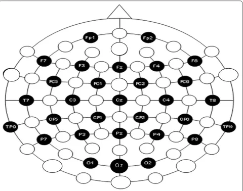
Participants were required to abstain from caffeine and nicotine (minimum of 3 hrs) and alcohol and drugs (be-ginning at midnight) prior to their test session. Upon arrival at the laboratory, they were seated in a sound-and light-attenuated chamber, where EEG recordings were obtained during 3 min vigilance-controlled eyes-closed (EC) and 3 min eyes-open (EO) resting conditions (counter-balanced). EEG was recorded (sampling rate 500 Hz) in reference to activity from electronically linked mastoids and using a cap system with 28 Ag/AgCl scalp electrodes (EasyCap, Herrsching-Breitbrunn, Germany) positioned on the scalp according to the 10–10 system [43] (Fig. 1). Electrodes placed on the external canthi and on the supra- and sub-orbital ridges recorded electrooculographic (EOG) activity, and an electrode at AFzserved as the ground. Electrode impedances were
maintained at≤5 kΩand electrical signals were recorded with amplifier bandpass filter settings of 0.1–80 Hz using a BrainVision Quickamp amplifier and BrainVision Re-corder Software (BrainVision, Richardson, TX, USA).
EEG processing
EEG data was processed off-line using BrainVision Analyzer Software (BrainVision, Richardson, TX, USA). Signals were referenced with electronically linked mastoid electrodes (TP9/10) or a scalp vertex (Cz) electrode to yield
two data sets for each of the EC and EO recordings. For both referenced recordings, signals were filtered (0.1– 30 Hz), ocular corrected [44], and segmented into 2 s epochs (50 % overlap). Subsequent automatic artifact rejection was used to exclude epochs with activity exceed-ing +/− 75 μV. The remaining epochs were visually inspected for additional artifacts and faulty channels. For each of EC and EO data sets (linked mastoid and Cz refer-ences), >100 s artifact-free signals from each of the 28 electrodes (TP9/10 was not used in the analyses) were
subjected to a Fast Fourier Transform (FFT) algorithm (Hanning window with 5 % cosine taper) for computation of both absolute and ln-transformed power (μV2) in delta (1–4 Hz), theta (4–8 Hz), alpha1, (8–10.5 Hz), alpha2
(10.5–13 Hz), alpha total (8–13 Hz) and beta (13–30 Hz) frequency bands.
Data mining
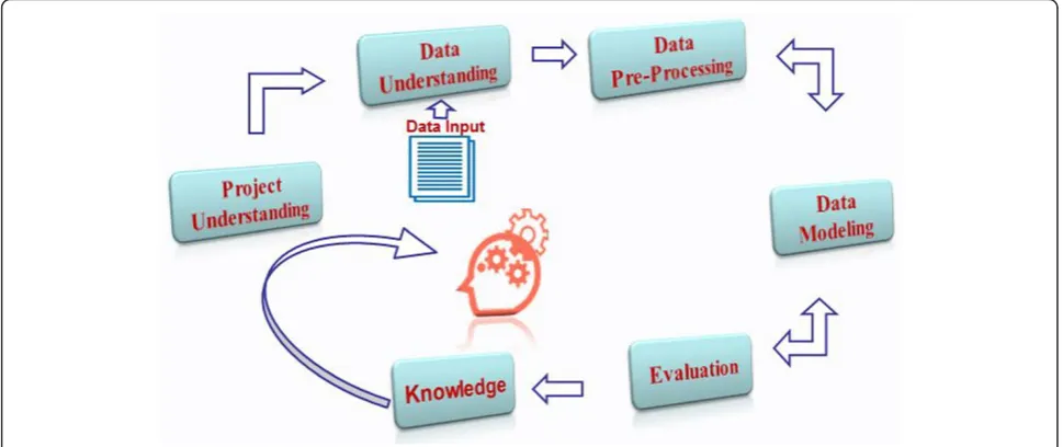
The Data Mining Methodology was chosen to provide an outline about the study’s life cycle to tackle the stated problem and to describe the processes, techniques and models involved in achieving the study’s goals. The methodology consists of six phases (Fig. 2), starting with the initial phase of understanding the project (Introduc-tion), followed by data understanding (EEG Acquisition/ Processing), data pre-processing, data modeling, evalu-ation and ending up with the deployment (knowledge discovery) [45]. The detailed description of each phase applied in this study is outlined below.
Data pre-processing
The data pre-processing phase includes all the tasks that are performed to construct and prepare the raw data into final datasets in order to be fed into the data model-ing phase [45]. The pre-processmodel-ing phase consisted of four main steps which are listed as follows:
Data cleaning The cleaning phase was performed in Microsoft Excel. Once the datasets were structured and examined for missing values, a small experiment was implemented to determine whether absolute or log power performed better. The results showed that the absolute power values yielded better accuracy compared with the log power values.
Data transformation Data transformation was performed by applying a normalization technique to make all the data values fall within a small range (0–1) to enable the efficient performance of the predictive model (clas-sifier). The employed normalization technique ismin-max normalization, which performs a linear transformation on the original data by setting the min value to 0 and max value to 1.“The minimum and maximum values are repre-sented in the formula (1) with minAand maxAof an
attri-bute A. Min-max normalization maps a value, viof A to vi’
in the range[new_maxA,new_minA]”[46].
v0 ¼ v−minA maxA−minAð
new maxA −new minAÞ
þnew minA
ð1Þ
Feature selection Genetic Algorithm (GA): This is a randomized search algorithm used to find an optimal solution for a problem via the process of natural selec-tion in data mining [47]. In GA, “chromosomes” are created randomly to represent the features of the data as genes. Each gene is assigned with a string of either 0 or
1, where 0 means the feature is not selected in that particular chromosome whereas 1 means the feature is selected [48]. For example, Fig. 3 represents a chromo-some created for EEG data for each band where genes reflect the 28 electrode sites.
Each chromosome represents a point in the search space and a number of chromosomes in the space are called a population. In GA, chromosomes are compared to each other to assess the goodness of each one in solving the problem. This is done by using the fitness function that evaluates and assigns a score for each
Table 1Data description
References Bands Condition Sites Frequencies Samples
Mastoids Alpha EO Fp1, Fp2, F3, F4, C3, C4, P3, P4, O1, O2, F7, F8, T7, T8, P7, P8, Fz, Cz, Pz, Oz, Fc1, Fc2, Cp1, Cp2, Fc5, Fc6, Cp5, Cp6
(8–10.5 Hz) HV 43
EC (10.5–13 Hz) MDD 53
Beta EO (13–30 Hz) HV 43
EC MDD 53
Theta EO (4–8 Hz) HV 43
EC MDD 53
Delta EO (1–4 Hz) HV 43
EC MDD 53
Cz Alpha EO Fp1, Fp2, F3, F4, C3, C4, P3, P4, O1, O2, F7, F8, T7, T8, P7, P8, Fz, Cz, Pz, Oz, Fc1, Fc2, Cp1, Cp2, Fc5, Fc6, Cp5, Cp6
(8–10.5 Hz) HV 43
EC (10.5–13 Hz) MDD 53
Beta EO (8–10.5 Hz) HV 43
EC (13–30 Hz) MDD 53
Theta EO (4–8 Hz) HV 43
EC MDD 53
Delta EO (1–4 Hz) HV 43
EC MDD 43
chromosome to select the best ones during the selection phase.
Fitness Function: In the fitness function, each chromo-some represents features that are selected by GA. Based on the selected features for each chromosome; a dataset is generated and is given to the predictive model (classi-fier) to evaluate the goodness of the chromosome. Be-fore feeding the classifier with the dataset, the dataset is mapped using Linear Discrimination Analysis (LDA) and then divided into training and testing sets. After that, the training set is fed into the decision tree (classifier) to build a classification model. Finally, the performance of the classifier is evaluated using the testing set to deter-mine how well the classifier performed by computing the accuracy. To assign the score for each chromosome, the fitness function is computed using the formula (2).
Fitness ¼ Accuracy−100 Number of selected features
Total number of feartures
ð2Þ
Based on the formula, the chromosomes which contain fewer features and provide higher detection rate will re-ceive a higher chance of selection for the next population.
Selection Operator (Tournament Selection): Each chromosome in the initial population goes through the same process as described above. Once all the chromo-somes are assigned scores, they are then compared with each other in order to select the best ones to reproduce the next population. In this study, theBinary Tournament Selection was used [48–51]. In the Binary Tournament Selection algorithm two chromosomes are first selected
randomly and based on their fitness function, the one that has a better fitness function is selected and a copy of that chromosome is sent to the next population. The selection algorithm repeats the same process until n samples are selected (nis number of samples in the initial population). Based on the proposed fitness function, the chromosomes that have higher fitness value will have a greater chance of being selected.
Crossover Operator (One-point): The selected popula-tion during the fitness funcpopula-tion needs to be reproduced to create a new generation of chromosomes for the next iteration. The crossover method is used to reproduce new chromosomes for the next population by selecting two parent chromosomes. From these, two new offspring chromosomes are produced by applying the crossover. For example in Fig. 4, parent chromosomes consist of 111010011 and 010111 001, the crossover method ran-domly chooses loci for exchanging between parents to create offspring with 111011001and 010110011[48–51]. Mutation Operator (Bit Flip): Another method that is employed to produce a new generation of chromo-somes is a Mutation, which randomly flips a bit in a single chromosome. For example, in the chromosome 111010011, the third locus is flipped to 110010011 [48].
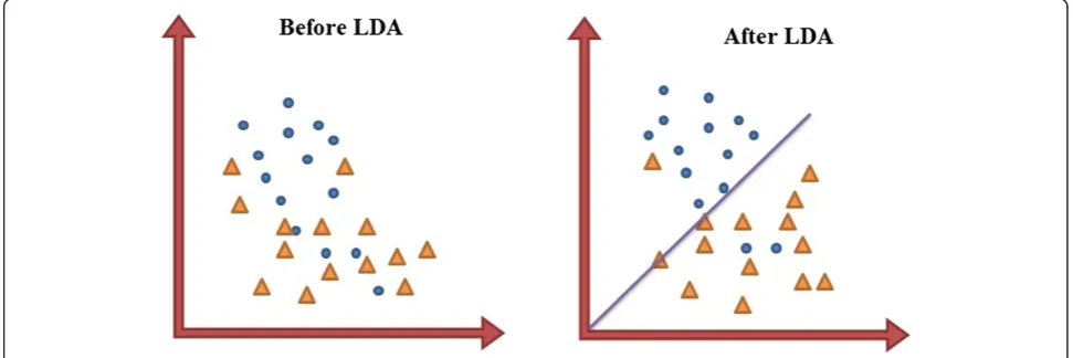
Feature mapping Linear Discriminant Analysis (LDA) is a method used in both feature mapping as well as a dimensional reduction and classification. LDA was used as a feature mapping method in order to transfer the original data into a new space where different classes can be discriminated linearly by finding a decision region
Fig. 3Chromosome representation
between the given classes in the newly mapped space that best maximizes the class separability [50]. Figure 5 shows a two dimensional dataset before and after applying LDA. With LDA, the features are mapped into a new feature space in which they are more linearly discriminant com-pared with the original feature.
LDA faces difficulties in cases of high dimensional data, where the LDA matrices are almost always singular [51]. In our dataset, in some experiments (e.g. Tables 6 & 7); there are more than 110 features while the training dataset consists of less than 100 samples. This indicates that it is not feasible to employ LDA directly on the data. Having observed the low performance of applying mere LDA on our datasets at the initial stage of the study, we decided to first employ GA to reduce the data dimension and then apply LDA to improve the accuracy of final classifier.
Once the four steps of the preprocessing phase were completed successfully, the datasets were ready to be classi-fied by applying the classification model described below.
Data modeling
A Decision Tree (DT) was the selected model for this study. Specifically, the C4.5 decision tree model was used. During the training phase, 70 % of the dataset was used to build a classification model that predicts the correct label of the testing set (consisting of the rest (30 %) of the datasets).
Data evaluation
The performance of the DT model was evaluated based on counting the test records that were correctly and incorrectly predicted by the DT. The Confusion Matrix provided information that allowed us to determine how well the model performed by computing the Accuracy for correct predictions andError Rate(ER) for incorrect predictions, sensitivity, specificity, positive and negative predicted values [52].
Data mining overview
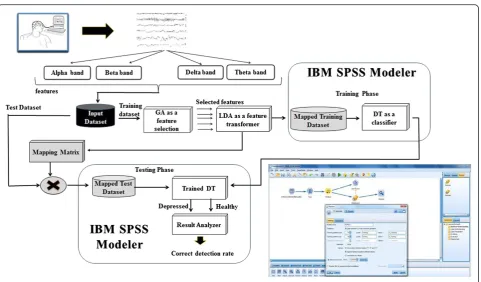
Before entering the cleansed and normalized data set into the feature selection phase using the GA, the datasets were divided into training (70 % of dataset) and testing (30 % of dataset) datasets, used for building a predictive model and testing the model’s performance, respectively. As described in Fig. 6, the input dataset contains the training set that is fed to the GA in order to select the best features that discriminate between HVs and MDD patients, and by applying the fitness function (explained in Feature selection). The best set of features was then transformed into a new space to linearly separate the data based on the classes by applying LDA. Subsequently, the training set was ready to build the Decision Tree for the predictive model. The features that were selected in the training were also selected in the testing set followed by applying LDA on the testing. Fi-nally, the mapped testing set was then fed into the trained decision tree to test if the model was able to pre-dict MDD patients from HVs and then performance of the model was measured using the accuracy and the error rate of the model (described in Data evaluation Evaluation Phase).
This approach was applied in two sets of analyses. The first was aimed at analyzing each frequency band indi-vidually during each of the EO and EC conditions (for
Fig. 5Linear discriminant analysis
Measurements Formula
Sensitivity : A/(A+ C)*100
Specificity : D/(D+ B)*100
Positive Prediction Value (PPV) : A/(A+ B)*100
Negative Prediction Value (NPV) : D/(D+ C)*100
Positive Likelihood Ratio (LR+) : Sensitivity/(100-Specificity)
Negative Likelihood Ratio (LR-) : (100-Sensitivity)/Specificity
each of the mastoid and Cz referenced datasets). Second, data from all bands were analyzed together during EO and EC conditions (for each of the mastoid and Cz refer-enced datasets). Both analyses were performed using MatlabandIBM SPSS Modeler.
Results
The datasets of the four bands (alpha, beta, delta and theta) during the EC and EO conditions were analyzed based on two views to determine the most accurate approach which might be: 1) Each band was analyzed individually during each condition EC and EO for each reference (Mastoid and Cz); and 2) The four bands (alpha, beta, delta and theta) were grouped together to be analyzed as one dataset in each condition EC and EO for Mastoid and Cz references.
Then, the testing dataset was used to validate the predictive model before and after applying GA and LDA. After that, the results were evaluated based on the Sensitivity, Specificity, Positive and Negative Like-lihood Rates (LR+ and LR-), Positive and Negative Predictive Values (PPV and NPV), accuracy, and Error rate for depressed and healthy individuals, see sec-tions Mastoid reference—bands analyzed individually, Cz reference—bands analyzed individually, Mastoid reference—bands analyzed together, and Cz reference— bands analyzed together for more details of the ana-lysis. In addition, Section Model evaluation presents the
results of the new obtained datasets, and it is used to evaluate the model that consists of the whole dataset that is used through Sections Mastoid reference—bands ana-lyzed individually, Cz reference—bands analyzed individu-ally, Mastoid reference—bands analyzed together, and Cz reference—bands analyzed together.
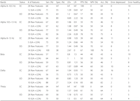
Mastoid reference—bands analyzed individually
The results of analyzing each band separately during the EO and EC conditions using a mastoid reference are pre-sented in Table 2. Apart from the delta band, classification error rates were relatively high as evidenced by accuracies ranging from 40–66 %. Low specificities were also noted in non-delta bands (range: 0–54 %). With more than half of the classifiers, sensitivity, specificity, Positive Likelihood Ratio (LR+) and NPV (Negative Predictive Value) rates increased following GA and LDA application but this was not necessarily associated with higher accuracy. Delta was the exceptional individual band classifier when analysed during EO. Although showing less than chance accuracy when analyzed with all candidate features, feature reduc-tion with GA and LDA markedly increased sensitivity, specificity and accuracy rates > 80 %. These results were accompanied by increases and decreases in LR+ and LR-, respectively. As displayed in “Additional file 1: Table S1” the specific scalp sites contributing to these findings were distributed over frontal, central and posterior regions of both hemispheres.
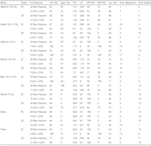
Cz reference—bands analyzed individually
The results of analyzing each band separately during the EC and EO conditions using a Cz reference are pre-sented in Table 3. Although sensitivity, PPV and NPV rates for some of the classifiers reached 100 %, with the exception of the alpha (8–10.5 Hz) band, accuracy rates associated with delta, theta and beta were relatively low (43–64 % over EO/EC conditions). Similarly modest accuracy and sensitivity rates (64 %) were observed with EC and EO alpha band analysis using all candidate features. However, GA and LDA feature extraction pro-cesses increased the EC alpha classifier’s sensitivity, PPV, NPV and accuracy rates to 94, 83, 90 and 86 %, re-spectively. Scalp recordings contributing to these clas-sifications were spread diffusely over frontal, central and parieto-occipital regions (“Additional file 1: Table S2”).
Mastoid reference—bands analyzed together
Table 4 presents the results of analyzing all of the bands together using either the total (8–13 Hz), or by separat-ing the low (8–10.5 Hz) or high (10.5–13 Hz) alpha band data during EO and EC conditions. Overall, accur-acy rates relying on all candidate features were relatively
low (56–64 %) but the classification accuracy of MDD patients and HVs significantly increased after feature selection with GA and LDA, regardless of whether alpha total (85–86 %), low (88–89 %) or high alpha band (80–86 %) features were used in the modeling. Of these, the best results were obtained when reduced EC low alpha features were used for classification yielding an accuracy rate approaching 90 %, high sen-sitivity and specificity rates (89 %), and LR+ (8.09) and LR- (0.12) values that strongly support this model for ruling-in and ruling-out depression. While the
“Additional file 1: Tables S3-S5” show that multiple recording regions contributed to these classifiers, left and right parietal and occipital recording sites (where alpha power is typically maximal) did not contribute to these results.
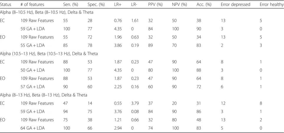
Cz reference—bands analyzed together
The results of the analysis of all the bands together using either the total (8–13 Hz), or by separating the low (8– 10.5 Hz) and high (10.5–13 Hz) alpha band data during EO and EC conditions are presented in Table 5.
Table 2Results- analysis of the individual bands- mastoid reference
Bands Status # of features Sen. (%) Spec. (%) LR+ LR- PPV (%) NPV (%) Acc. (%) Error depressed Error healthy
Alpha 8–10.5 Hz EC 28 Raw Features 64 Inf Inf Inf 100 0 64 0 10
12 (GA + LDA) 71 55 1.29 0.65 67 50 61 6 5
EO 28 Raw Features 75 63 1.2 0.67 17 90 43 15 1
15 (GA + LDA) 56 80 0.69 2.22 56 20 43 8 8
Alpha 10.5–13 Hz EC 28 Raw Features 67 63 1.06 0.9 33 70 46 12 3
11 (GA + LDA) 67 62 1.08 0.87 56 50 54 8 5
EO 28 Raw Features 77 53 1.44 0.49 56 70 61 8 3
10 (GA + LDA) 82 36 2.26 0.28 78 70 75 4 3
Alpha 8–13 Hz EC 28 Raw Features 64 65 0.98 1.03 39 60 46 11 4
5 (GA + LDA) 73 59 1.24 0.66 44 70 54 10 3
EO 28 Raw Features 77 53 1.44 0.49 56 70 61 8 3
14 (GA + LDA) 100 38 2.67 0 67 100 79 6 0
Beta EC 28 Raw Features 57 71 0.8 1.5 44 40 43 6 10
10 (GA + LDA) 64 64 1 1 50 50 50 9 5
EO 28 Raw Features 59 73 0.81 1.51 56 30 46 7 8
11 (GA + LDA) 67 63 1.07 0.89 44 60 50 10 4
Delta EC 28 Raw Features 67 64 1.04 0.93 11 90 39 16 1
18 (GA + LDA) 56 75 0.75 1.75 50 30 43 9 7
EO 28 Raw Features 58 69 0.85 1.33 39 50 43 11 5
10 (GA + LDA) 88 27 3.24 0.16 83 80 82 2 3
Theta EC 28 Raw Features 64 Inf Inf Inf 100 0 64 0 10
18 (GA + LDA) 79 50 1.57 0.43 61 70 64 7 3
EO 28 Raw Features 69 58 1.18 0.75 61 50 57 7 5
As shown with mastoid-referenced analyses, analyz-ing all bands together usanalyz-ing total raw features of Cz referenced EEG yielded low diagnostic accuracy rates
between 31–64 % across EO and EC behavioural
states. Similarly, feature extraction with GA and LDA elevated accuracies with total alpha (EC/EO: 86, 83 %), low alpha (EC/EO: 90, 83 %), and high alpha (EC: 88 %) analyses. Further, the more robust classifi-cations were seen in the analysis conducted with reduced low alpha features under the EC condition which also resulted in sensitivity and NPV rates of 100 %, along with moderate rates of specificity (77 %), LR+ (4.35) and LR-(0). The scalp regions contributing to the low alpha
classifier were relatively widespread (Additional file 1: Tables S3-S5”).
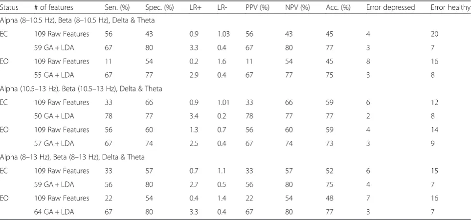
Model evaluation
Tables 6 and 7 present the results when newly recorded (unseen) EEG recordings are analyzed using all the bands using mastoid or Cz references, and with low, high or total alpha band features.
Although accuracy was frequently below 60 % for mastoid and Cz referenced datasets using all candidate features, classification rates improved to > 70 % using the reduced features derived with GA and LDA. Accuracy reached 75–77 % levels with EC and EO Cz referenced
4 (GA + LDA) 64 Inf Inf Inf 100 0 64 0 10
EO 28 Raw Features 64 Inf Inf Inf 100 0 64 0 10
9 (GA + LDA) 74 44 1.66 0.47 78 50 68 4 5
Alpha 8–13 Hz EC 28 Raw Features 64 Inf Inf Inf 100 0 64 0 10
7 (GA + LDA) 100 57 1.77 0 28 100 54 13 0
EO 28 Raw Features 64 Inf Inf Inf 100 0 64 0 10
9 (GA + LDA) 100 52 1.91 0 39 100 61 11 0
Beta 8–10.5 Hz EC 28 Raw Features 58 69 0.85 1.33 39 50 43 10 5
8 (GA + LDA) 62 67 0.92 1.15 44 50 46 11 5
EO 28 Raw Features 58 69 0.85 1.33 39 50 43 10 5
9 (GA + LDA) 75 63 1.2 0.67 17 90 43 15 1
Beta 10.5–13 Hz EC 28 Raw Features 59 73 0.81 1.51 56 30 46 8 7
8 (GA + LDA) 100 44 2.25 0 56 100 71 0 8
EO 28 Raw Features 62 100 0.62 Inf 89 0 57 2 10
11 (GA + LDA) 74 44 1.68 0.46 78 50 68 4 5
Beta 8–13 Hz EC 28 Raw Features 64 0 0.64 Inf 100 0 64 0 10
10 (GA + LDA) 64 0 0.64 Inf 100 0 64 0 10
EO 28 Raw Features 64 0 0.64 Inf 100 0 64 0 10
10 (GA + LDA) 83 70 2.77 0.24 83 70 79 3 2
Delta EC 28 Raw Features 64 0 0.64 Inf 100 0 64 0 10
9 (GA + LDA) 64 0 0.64 Inf 100 0 64 0 10
EO 28 Raw Features 64 0 0.64 Inf 100 0 64 0 10
10 (GA + LDA) 80 61 1.31 0.51 90 22 46 14 1
Theta EC 28 Raw Features 64 0 0.64 Inf 100 0 64 0 10
9 (GA + LDA) 100 57 1.77 0 28 100 54 13 0
EO 28 Raw Features 77 53 1.44 0.49 56 70 61 8 3
EEG, but the maximal 80 % accuracy was evidenced with EO low alpha analysis, which also yielded sensi-tivity and specificity rates of 77 % and 80 %, respect-ively, together with relatively high PPV (78 %) and NPV (80 %) values.
As indicated in Tables 6 and 7, the model shows an acceptable performance on the newly recorded data. The accuracy of the model fluctuates between 70 % and 80 %. For example, based on the Cz reference, EC data-set with all bands (Table 7), the accuracy of the model
on 106 raw features is about 60 %, while by applying the proposed method, the accuracy reaches 72.7 % which is a noticeable improvement.
Discussion
The heterogeneity of symptom profiles and severity among patients with MDD is a major challenge for diag-nostic classification. Further, given the reliability prob-lems associated with subjective assessments of clinical phenomena there is an increasing effort to identify more
Table 4Mastoid reference results (For around 28 records)
Status # of features Sen. (%) Spec. (%) LR+ LR- PPV (%) NPV (%) Acc. (%) Error depressed Error healthy
Alpha (8–10.5 Hz), Beta, Delta & Theta
EC 112 Raw Features 69 43 1.21 0.72 53 60 56 8 4
60 GA + LDA 89 89 8.09 0.12 94 80 89 1 2
EO 112 Raw Features 68 50 1.36 0.64 83 30 64 3 7
58 GA + LDA 94 75 3.76 0.08 83 90 88 3 1
Alpha (10.5–13 Hz), Beta, Delta & Theta
EC 112 Raw Features 73 78 3.32 0.35 80 70 75 2 3
46 GA + LDA 77 100 Inf 0.23 100 70 86 0 3
EO 112 Raw Features 62 71 2.14 0.54 80 50 65 2 5
42 GA + LDA 80 80 4 0.24 80 80 80 2 2
Alpha (8–13 Hz), Beta, Delta & Theta
EC 112 Raw Features 62 33 0.93 1.15 76 20 56 4 8
60 GA + LDA 88 80 4.4 0.15 88 80 85 2 2
EO 112 Raw Features 67 40 1.12 0.83 67 40 57 6 6
58 GA + LDA 94 75 3.76 0.08 83 90 86 3 1
Table 5Cz reference results
Status # of features Sen. (%) Spec. (%) LR+ LR- PPV (%) NPV (%) Acc. (%) Error depressed Error healthy
Alpha (8–10.5 Hz), Beta (8–10.5 Hz), Delta & Theta
EC 109 Raw Features 55 28 0.76 1.61 32 50 38 13 5
59 GA + LDA 100 77 4.35 0 84 100 90 3 0
EO 109 Raw Features 55 72 1.96 0.63 32 50 34 13 5
55 GA + LDA 85 78 3.86 0.19 89 70 83 2 3
Alpha (10.5–13 Hz), Beta (10.5–13 Hz), Delta & Theta
EC 109 Raw Features 88 53 1.87 0.23 47 90 64 8 1
50 GA + LDA 100 77 4.35 0 80 100 88 3 0
EO 109 Raw Features 88 53 1.87 0.23 47 90 64 8 1
57 GA + LDA 90 60 2.25 0.16 60 90 72 6 1
Alpha (8–13 Hz), Beta (8–13 Hz), Delta & Theta
EC 109 Raw Features 47 14 0.55 3.79 37 20 31 12 8
59 GA + LDA 94 75 3.76 0.08 84 90 86 3 1
EO 109 Raw Features 75 38 1.21 0.66 32 80 48 13 2
brain-based, objective and reliable classifiers for various psychiatric disorders, including depression. In this paper, classification approaches were performed on EEG signal features (power density in different frequency bands) derived from multiple scalp recording sites, during two states (EO/EC) and analyzed using two reference mon-tages. In Experiment 1, individual bands resulted in relatively high classification errors, regardless of whether or not the complexity and redundancy of signal features was reduced by the genetic algorithm. Exceptions were observed with EO mastoid-referenced delta and EC Cz-referenced total alpha, with the reduced extracted
features of each band exhibiting > 80 % accuracy, sen-sitivity and PPVs. These latter findings are generally supportive of previous group-level comparison studies showing activity of alpha, and to a lesser extent delta oscillations to distinguish depressed and healthy vol-unteer samples [26].
When analyzing each band separately, classification was similarly less than optimal in Experiment 2 when bands were analyzed together and with the total set of candidate features, but was markedly increased following feature reduction. Regardless of the type of reference (mastoid vs. Cz) or vigilance state (EC vs. EO), most
Alpha (10.5–13 Hz), Beta, Delta & Theta
EC 112 Raw Features 56 60 1.3 0.7 56 60 59 4 14
46 GA + LDA 78 69 2.4 0.3 78 69 70 2 11
EO 112 Raw Features 44 66 1.2 0.8 44 66 61 5 12
42 GA + LDA 67 74 2.5 0.4 67 74 73 3 9
Alpha (8–13 Hz), Beta, Delta & Theta
EC 112 Raw Features 33 57 0.7 1.1 33 57 52 6 15
60 GA + LDA 78 77 3.4 0.2 78 77 77 2 8
EO 112 Raw Features 56 43 0.9 1.03 56 43 45 4 20
58 GA + LDA 67 74 2.5 0.4 67 74 73 3 9
Table 7Cz Reference Results on the new unseen 44 records
Status # of features Sen. (%) Spec. (%) LR+ LR- PPV (%) NPV (%) Acc. (%) Error depressed Error healthy
Alpha (8–10.5 Hz), Beta (8–10.5 Hz), Delta & Theta
EC 109 Raw Features 56 43 0.9 1.03 56 43 45 4 20
59 GA + LDA 67 80 3.3 0.4 67 80 77 3 7
EO 109 Raw Features 11 54 0.2 1.6 11 54 45 8 16
55 GA + LDA 67 77 2.9 0.4 67 77 75 3 8
Alpha (10.5–13 Hz), Beta (10.5–13 Hz), Delta & Theta
EC 109 Raw Features 33 66 0.9 1.01 33 66 59 6 12
50 GA + LDA 78 77 3.4 0.2 78 77 77 2 8
EO 109 Raw Features 56 60 1.3 0.7 56 60 59 4 14
57 GA + LDA 67 74 2.5 0.4 67 74 73 3 9
Alpha (8–13 Hz), Beta (8–13 Hz), Delta & Theta
EC 109 Raw Features 33 57 0.7 1.1 33 57 52 6 15
59 GA + LDA 56 80 2.7 0.5 56 80 75 4 7
EO 109 Raw Features 22 54 0.4 1.4 22 54 48 7 16
models exhibited low classification errors, with high accuracy and sensitivity values. The electrode sites con-tributing to these classifiers and the above-mentioned single band delta and alpha classifiers were widely dis-tributed across frontal, temporal and posterior regions in both hemispheres. These data are consistent with func-tional neuroimaging studies that tend to characterize depression as a dysfunction in a network(s) of discrete, but functionally integrated, cortico-limbic pathways [53], which can be assessed by brain-based algorithms for diagnosis and optimized treatment [54, 56].
In summary, the most accurate decision tree models (accuracies > 80 %) were evaluated with unseen data from 44 participants, including 35 HVs and 9 MDD patients. Correct diagnosis rates of the models were found to be quite accurate. These results generally support the notion that data mining techniques, and especially those involv-ing feature extraction, may yield promisinvolv-ing classifiers for the EEG signal processing applications, specifically in cases of MDD and control subjects classification. Improved classification accuracies may possibly be achieved with the addition of other candidate features besides EEG power including EEG coherence and cordance measures, which have been reported to distinguish de-pressed patients from healthy volunteers, and the EEG antidepressant response (ATR) index, which has predicted treatment response in depressed patients [26, 27].
Conclusions
In this study we demonstrated that data mining applied to EEG signals may be a useful tool in discriminating between depressed and healthy individuals. Given the questionable reliability of diagnoses based on clinical symptoms, this quantitative methodology may be a useful adjunctive clinical decision support for identifying depres-sion and it supports independent studies confirming the potential clinical utility of computer-aided diagnosis of depression using EEG signals [55].
Additional file
Additional file 1: Table S1.Feature Selection—Individually Analyzed Mastoid Referenced EEG Bands.Table S2.Feature Selection—Individually Analyzed Cz Referenced EEG Bands.Table S3.Feature Selection—Combined Analyzed Bands Using the Low (8–10.5) Hz) Alpha EEG Band.Table S4. Feature Selection—Combined Analyzed Bands Using the High (10.5–13 Hz) Alpha EEG Band.Table S5.Feature Selection—Combined Analyzed Bands Using the Total (8.5–13 Hz) Alpha EEG Band. (DOCX 44 kb)
Abbreviations
DSM-5:Diagnostic and Statistical Manual of Mental Disorders, 5th edition; DT: Decision tree; EEG: Electroencephalography; FFT: Fast Fourier Transform; fMRI: Functional magnetic resonance imaging; GA: Genetic algorithm; LDA: Linear Discriminant analysis; LR+: Positive Likelihood Ratio; LR-: Negative Likelihood Ratio; MADRS: Montgomery-Asberg Depression Rating Scale; MDD: Major depressive disorder; NPV: Negative Predictive Value;
PET: Positron emission tomography; PPV: Positive Predictive Value; SCID: Structured Clinical Interview for DSM.
Competing interests
None of the authors have any financial or non-financial competing interests related to this paper.
Authors’contributions
VK was one of the authors responsible for developing the research questions and overseeing the project, and helped to draft the manuscript, particularly the Introduction, Methods (Sections Project participants, EEG acquisition and EEG processing), and Discussion. BR was also responsible for developing and overseeing the project, directing, overseeing and interpreting the data mining results and helped to interpret the data and edit the manuscript. PB, the psychiatrist on the project, screening, interviewed and diagnosed all patients and helped to edit the paper. GR was involved in the conception of the project, coordinated the communications/interactions between investigators and submitting the project for funding and was involved in editing the manuscript. MM and FA were responsible for performing the data mining procedures, writing results sections and editing the manuscript. NJ recruited and tested the patients and controls and processed all the EEG files and assisted in editing the manuscript. DS and SD prepared and assembled EEG and clinical data files and assisted in editing the manuscript. All authors have given approval for this manuscript to be published.
Acknowledgements
This research was supported by MITACS Canada Grant # IT02932, and The IBM center for Business Analytics and Performance at the University of Ottawa, Canada.
Author details
1Knowledge Discovery and Data mining Lab (KDD), University of Ottawa, Ottawa, ON, Canada.2Department of Psychiatry, McGill University, Montreal, QC, Canada.3Department of Cellular and Molecular Medicine, University of Ottawa, Ottawa, ON, Canada.4School of Psychology, University of Ottawa, Ottawa, ON, Canada.5Institute of Mental Health Research at the Royal Ottawa Mental Health Care Centre, University of Ottawa, 1145 Carling Avenue, Ottawa, ON K1Z 7 K4, Canada.
Received: 21 May 2015 Accepted: 8 December 2015
References
1. Kessler R, Chiu W, Demier U, Merikangas K, Walters E. Prevalence, severity, and comorbidity of 12-month DSM-IV disorders in the National Comorbidity Survey Replication. Arch Gen Psychiatry. 2015;62:617–27.
2. Yach D, Hawkes C, Gould C, Hofman K. The global burden of chronic disorders: Overcoming impediments to prevention and control. JAMA. 2004;291:2616–22.
3. Murray T, Vos T, Lozano R, Naghavi M, Flaxman AD, Michaud C, et al. Disability-adjusted life years (DALYs) for 291 diseases and injuries in 21 regions, 1990–2010: A systematic analysis for the global burden of disease study. Lancet. 2010;380:2197–223.
4. Olesen J, Gustavsson A, Svensson M, Wittchen U, Jonsson B. The economic cost of brain disorders in Europe. Eur J Neurol. 2012;19:155–62.
5. American Psychiatric Association. Diagnostic and Statistical Manual of Mental Disorders. 5th ed. Arlington: American Psychiatric Publishing; 2013. 6. Halaris A. A primary focus on the diagnosis and treatment of major
depressive disorder in adults. J Psychiatr Pract. 2011;17:340–50. 7. Biomarkers Definitions Working Group. Biomarkers and Surrogate
endpoints: Preferred definitions and concept framework. Clin Pharmacol Ther. 2001;69:89–95.
8. Insel T, Cuthbert B, Garvey M, Heinssen R, Pine DS, Quinn K, et al. Research Domain Criteria (RDoC): Toward a new classification framework for research on mental disorders. Am J Psychiatry. 2010;167:748–51.
9. Enaw E, Smith A. Biomarker development for brain-based disorders: Recent progress in psychiatry. J Neurol Psychol. 2013;1:7.
10. Fu C, Costafreda S. Neuroimaging-based biomarkers in psychiatry: Clinical opportunities of a paradigm shift. Can J Psychiatry. 2013;58:499–508. 11. Hasler G, Drevets W, Manji H, Charney D. Discovering endophenotypes for
utility of neuroimaging in depression: An overview. Neurophsychiatr Dis Treat. 2014;10:1509–22.
17. Ritsner M, Gottesman E. Where do we stand in the quest for
neuropsychiatric biomarkers and what next? Chapter 1. In: The Handbook of Neuropsychiatric Biomakrers, Endophenotypes and Genes. New York: Springer; 2009. p. 3–17.
18. Michel C, Murray M. Towards the utilization of EEG as a brain imaging tool. Neuroimage. 2012;61:371–85.
19. Leiser S, Dunlop J, Bowlby M, Devilbiss D. Aligning strategies for using EEG as a surrogate biomarker: A review of preclinical and clinical research. Biochem Pharmacol. 2011;81:1408–21.
20. Knott V. Quantitative EEG, methods and measures in human
psychopharmacological research. Hum Psychopharmacol. 2000;15:479–98. 21. Kemp A, Gordon E, Rush A, Williams L. Improving the prediction of
treatment response in depression: Integration of clinical, cognitive, psychophysiological, neuroimaging, and genetic measures. CHS Spectr. 2008;13:12.
22. Leuchter A, Cook J, Hamilton S, Narr K, Toga A, Hunter A, et al. Biomarkers to predict antidepressant response. Curr Psychiatr Rep. 2010;12:553–62. 23. Leuchter A, Cook I, Hunter A, Korb A. A new paradigm for the prediction of
antidepressant treatment response. Dialogues Clin Neurosci. 2009;11:435–46. 24. MacQueen G. Neuroimaging and electrophysiology in predicting treatment
responsiveness in depression: Bridging the lab-to-clinic divide? Can J Psychiatry. 2013;58:497–8.
25. Jaworska N, Protzner A. Electrocortical features of depression and their clinical utility in assessing antidepressant treatment outcome. Can J Psychiatry. 2013;58:509–14.
26. Alhaj H, Wisniewski G, McAllister-Williams R. The use of the EEG in measuring therapeutic drug action: Focus on depression and antidepressants. J Psychopharmacol. 2011;25:1175–91.
27. Baskaran A, Milev R, McIntyre R. The neurobiology of the EEG biomarker as a predictor of treatment response in depression. Neuropharmacol. 2012;63:507–13.
28. Leuchter A, Cook I, Hunter A, Korb A. The use of clinical neurophysiology for the selection of medication in the treatment of major depressive disorder: The state of the evidence. Clin EEG Neurosci. 2009;40:78–83. 29. Lemm S, Blankertz B, Dickhaus T, Muller K. Introduction to machine learning
for brain imaging. Neuroimage. 2011;56:387–99.
30. Pereira F, Mitchell T, Botvinick M. Machine learning classifiers and fMRI: A tutorial overview. Neuroimage. 2009;45:5199–209.
31. Ahmadlou M, Adeli H, Adeli A. Fractality analysis of frontal brain in major depressive disorder. Int J Psychophysiol. 2012;85:206–11.
32. Hosseinifard B, Moradi M, Rostami R. Classifying depression patients and normal subjects using machine learning techniques and nonlinear features from EEG signals. Comp Meth Prog Med. 2013;109:339–45.
33. Khodayari-Rostamabad A, Reilly J, Hasey G, de Bruin H, MacCrimmon D. Diagnosis of psychiatric disorders using EEG data and employing a statistical decision model. Conf Proc IEEE Eng Med Biol Soc. 2010;2010:4006–9.
34. Knott V, Mahoney C, Kennedy S, Evans K. EEG power, frequency, asymmetry and coherence in male depression. REs Psychiatry Neuroimag. 2001;106:123–40.
35. Li YJ, Fan FY. Classification of schizophrenia and depression by EEG and ANNs. Conf Proc IEEE Eng Med Biol Soc. 2005;3:2679–82.
36. Barry R, Clarke A, Johnstone S, Magee CA, Rushby JA. EEG differences between eyes-closed and eyes-open resting conditions. Clin Neurophysiol. 2007;118:2205–23.
37. Tan B, Kong X, Yang P, Jin Z, Li L. The difference of brain functional connectivity between eyes-closed and eyes-open using graph theoretical analysis. Comput Math Menthods Med. 2013;2013:976365.
topographic studies of spontaneous and evoked EEG activity. Am J EEG Technol. 1985;25:83–92.
44. Gratton G, Coles M, Donchin E. A new method for off-line removal of ocular artifact. Electroencephalogr Clin Neurophysiol. 1983;55:468–84.
45. Shearer C. The CRISP-DM model: The new blueprint for data. J Data Warehouse. 2000;5:13–22.
46. Han J, Kamber M. Data Mining: Concepts and Techniques. 2nd ed. San Francisco: Morgan Kaufmann; 2006.
47. Thede SM. An introduction to genetic algorithms. J Circuits Syst Comput. 2004;20:115–23.
48. Mitchell M. An Introduction to Genetic Algorithms. London: MIT Press; 1998. 49. Eiben A, Smith JE. Introduction to Evolutionary Computing. 2nd ed. Berlin:
Springer; 2007.
50. Mohammadi M, Raahemi B, Akbari A, Nassersharif B, Moeinzadeh H. Improving linear discriminant analysis with artificial immune 3 system-based evolutionary algorithms. J Inf Sci. 2011;189:219–32.
51. Yu H, Jie Y. A direct LDA algorithm for high-dimensional data with application to face recognition. Pattern Recogn. 2001;34:2067–70. 52. Tan PN, Steinbach M, Kumar V. Introduction to Data Mining. Boston:
Pearson Addison-Wesley; 2006.
53. Mayberg H. Limbic-cortical dysregulation: A proposed model of depression. J Neuropsychiat. 1997;9:47–481.
54. Mayberg H. Modulating dysfunctional limbic-cortical circuits in depression: Towards development of brain-based algorithms for diagnosis and optimised treatments. Br Med Bull. 2003;65:193–207.
55. Acharya U, Sudarshan V, Adeli H, Santhosh J, Koh J, Adeli A. Computer-aided diagnosis of depression using EEG signals. Eur Neurol. 2015;73:329–36. 56. Labermaier C, Masana M, Muller M. Biomarkers predicting
antidepressant treatment response: How can we advance the field? Dis Markers. 2013;35:23–31.
• We accept pre-submission inquiries
• Our selector tool helps you to find the most relevant journal
• We provide round the clock customer support
• Convenient online submission
• Thorough peer review
• Inclusion in PubMed and all major indexing services
• Maximum visibility for your research
Submit your manuscript at www.biomedcentral.com/submit