RESEARCHARTICLE
Twitter location (sometimes)
matters: Exploring the relationship
between georeferenced tweet
content and nearby feature classes
Stefan Hahmann
1, Ross S. Purves
2, and Dirk Burghardt
11
Institute for Cartography, Dresden University of Technology, Germany 2Department of Geography, University of Zurich-Irchel, Zurich, Switzerland
Received: June 18, 2014; returned: August 7, 2014; revised: August 27, 2014; accepted: September 22, 2014.
Abstract: In this paper, we investigate whether microblogging texts (tweets) produced on
mobile devices are related to the geographical locations where they were posted. For this purpose, we correlate tweet topics to areas. In doing so, classified points of interest from OpenStreetMap serve as validation points. We adopted the classification and geolocation of these points to correlate with tweet content by means of manual, supervised, and unsuper-vised machine learning approaches. Evaluation showed the manual classification approach to be highest quality, followed by the supervised method, and that the unsupervised clas-sification was of low quality. We found that the degree to which tweet content is related to nearby points of interest depends upon topic (that is, upon the OpenStreetMap category). A more general synthesis with prior research leads to the conclusion that the strength of the relationship of tweets and their geographic origin also depends upon geographic scale (where smaller scale correlations are more significant than those of larger scale).
Keywords: correlation between location and content, mobile microblogging, natural
lan-guage processing, data mining, Twitter, OpenStreetMap
1
Introduction
brought with it a wealth of potential opportunities for data-driven research. A common observation with respect to such data is that they often come with an implicit or explicit georeference [35], and thus can be used to explore research questions of a geographical nature, such as the spread of flu [38, 59], the locations and magnitudes of earthquakes [54], the nature of landmarks photographed and preferred by individuals [1, 16, 31], or even the prediction of elections [13, 62]. However, a healthy skepticism has also developed with respect to the true properties and meaning of this data (e.g., [26, 35]) as it has become clear that the data does not, and indeed cannot speak itself.
In this paper we seek to contribute to this debate by exploring one commonly made assumption. Microblogging services, such as Twitter, are seen by many researchers as an excellent opportunity to link text to locations (e.g., [2,12,29,41,56,67]), especially where the information is sent from a mobile device and directly associated with coordinates. How-ever, it is equally obvious that one doesn’t need to be at the location of an earthquake to discuss or react to it, and in this paper we aim to explore the extent to which the content of microblogging texts relate to the locations from which they are sent. Our underlying hypothesis is that if it is possible to extract meaningful geographical patterns from mi-croblogging texts, then it should also be possible to relate such texts to existing geographic context. If the latter is not the case, this would in turn suggest that patterns emerging from such data may be more strongly influenced by the underlying distribution of the data source rather than any process controlling variation in the locations of the content itself.
The above hypothesis leads us to the overarching research question addressed in this paper, which can be simply stated as follows:
To what degree are the contents of individual microblogging texts related to their loca-tion?
In order to explore this question in more detail, we identify the following set of detailed research questions which we will explore in the remainder of the paper:
(1) How can we represent spatial context in order to investigate the relationship between the information content and its surroundings?
(2) How can individual texts be classified such that content can be related to surround-ings?
(3) Can we automate this classification process by means of machine learning? (4) Which learning algorithms would be best suited for such kind of automation? (5) Is there a corpus that allows us to appropriately substitute manual training data for
the classification task?
(6) Does the proportion of texts related to location-specific information show a decay over distance—in other words are the locations of the texts which relate to specific locations non-randomly distributed in space?
1.1
Organization of the paper
2
State of the art
2.1
Twitter as a research corpus
In recent years, microblogging has evolved into a key means of communicating both within the World Wide Web (WWW) and in the broader sphere of social media [32, 71] (for exam-ple, microblog contents are often displayed or reported in traditional print and audiovisual media and used as ways to elicit audience responses). Microblogs are so-called because of their terse, but publicly available content which can usually be associated with an individ-ual, and are published on the WWW. Twitter is perhaps the most famous example of such a service, with its 140 character limit. Characteristic features of this type of text are often the expression of subjective impressions, trivia, opinions, and information [32]. The style of the texts is dominated by abbreviations, the use of hashtags indicating particular themes, (internet) slang and spelling mistakes [28, 37].
As well as Twitter, other microblogging platforms exist such as Tumblr and Weibo, with similar services being provided by Facebook, LinkedIn, and GooglePlus. As Twitter is currently the microblogging platform with the largest number of active users, especially in our study area, we use texts that are published via this service as a research corpus in this paper.
The sum of all published microblogging texts (tweets) may collectively be considered a source of information about opinions and sentiments on products, politics, society, and events. There are many approaches, typically focused on some form of natural language processing (NLP), to the automated analysis of such texts. Metaxas and Mustafaraj [46] re-view applications for which the potential of an automated analysis of microblogging texts has been investigated. Examples include prediction of box-office revenues for movies [4], stock markets fluctuations [8], flu outbreaks [38, 59], and even (political) elections [13, 62], though the debate over the latter application demonstrates that some claims should be treated with care [23, 33]. Moreover, the so-called “Twittersphere” may be used in order to analyze opinions and sentiments by means of sentiment analyses [61]. In this context, the correlation between the results of such analyses and events has also been investigated [40] and it has been argued that, for instance, for the purpose of disaster management, mi-croblogging texts can support the decision support. Examples of research in this domain includes work addressing fire [19, 34, 64], floods [73], and earthquakes [54].
Besides such potential applications, the socio-economic characteristics of the Twitter user community have been explored. It has been shown that the intensity of the usage of the service within a specific region correlates with the average income and education of the population within this region [43]. With regard to the main intentions of usage it has been found that daily chatter, conversations, sharing information, and reporting news dominate [32]. This taxonomy has been confirmed in a second study which found user status updates, private conversations, weblinks to blogs and news, politics, sports, events, and advertising to be the main Twitter message types [17].
2.2
Relationship of geographic location and content of microblog-texts
Figure 1: Visualization of term frequencies, after stop word filtering, in mobile generated tweets in the center of Dresden.
IP-address of the user, the current cell site location of the user, or via the GPS module of the mobile device. We call tweets for which this meta-information is availablegeoreferenced tweets.
Some of the tweets that do not have position meta-information may be automatically georeferenced based on the actual text. However, due to the short length of the texts there is usually a lack of context, which makes text-based georeferencing challenging. Never-theless, in previous work it has been shown that by using the correlation between text content and the locations, where they have been created, it is possible to approximate posi-tion [12, 29, 56, 67]. The methods that are applied for this purpose use toponyms contained in the texts as well as words that are characteristic for specific regions, such as the word “beach” for a coastal region. However, the average positioning accuracy that has been reached by these methods—480km in [67], 800km in [12], 1400km in [56], and federal state accuracy in [29]—is limited and only appropriate for low resolution applications. Likewise, this proves a correlation between location and contents only for small scales.
These findings suggest the assumption that the correlation between microblog-contents and the locations where they have been created depends on the resolution of the analysis. This assumption is further supported by visualization of term frequencies derived from mobile generated texts in the area of Dresden that we show in Figure 1. It can be seen that the toponym “Dresden” is very frequent, suggesting that many tweets in this area do indeed refer to the city of Dresden.
that Twitter users more often refer to toponyms near to the home locations that they have specified in their user profiles.
2.3
Classification of microblogging texts by natural language processing
The classification of information simplifies the retrieval of information that is relevant to specific tasks. Methods of computational linguistics may support the classification of in-formation in natural language texts. These methods often apply supervised machine clas-sification, whose approaches are based on machine learning. They are well-established in the field and have already been implemented for a number of application areas including spam detection [3] and sentiment analyses [51, 52].
All supervised machine classification methods need training data to derive decision criteria supported by statistical procedures. In the field of computational linguistics docu-ments classified by humans are typically used as training data. Figure 2 illustrates schemat-ically the process of supervised text classification with the help of manually classified doc-uments. There are multiple alternatives for the actual classification algorithm. The most common algorithms are based on statistical procedures, whose aim it is to approximate class probability distributions from the training data. These distributions aim to classify new texts by deriving the probabilities for all possible classes, and subsequently selecting the class with the highest probability [10].
Unclassified documents
Classified documents
Training data as input For machine learning
Feature vectors
Classification algorithm
(e.g.: Naive Bayes, Maximum Entropy)
Probability function Decision criteria
Automated Text classification
Training documents
Manual Classification
Figure 2: Schematic representation of supervised text classification using manually classi-fied training data (figure is an adaptation of Scharkows’ illustration [55]).
the number of documents within the whole corpus that contain a specific word. Higher n-gram statistics, such as bin-gram or trin-grams, are also possible, but require larger training sets, since otherwise too many unique features which are never repeated prevent documents from being automatically classified.
Hence, the result of the learning process of each algorithm is a model, which contains the features, i.e., the words, and the corresponding weights, i.e., probabilities, for each possible class. Three of the most common text classification algorithms in the field of ma-chine learning are naive Bayes (NB), maximum entropy (ME), and support vector mama-chines (SVM) all of which apply a “bag of words” approach. While this sort of approach to text classification does not consider grammar and qualifying information, such as negation and comparison, they have a correspondingly low implementation complexity. A comparison of all three algorithms in the field of text classification is presented by Pang and Lee [52], who explore the example of sentiment classification. As we will use NB and ME in our empirical study, we will introduce these two algorithms in further detail in the following.
2.3.1 Naive Bayes
Naive Bayes classification is based on Bayes’ theorem of conditional probability. With re-gard to the automatic classification of documents the concrete question is, what is the prob-ability that a document containing a specific word belongs to a specific class. The proba-bility function is derived by analyzing relative word frequencies in the training data. For details on the computation of naive Bayes classification, readers are advised to consult, e.g., Scharkow [55]. An overview of applications of naive Bayes in the field of computational linguistics is compiled by Lewis [42]. The Bayes’ classification is callednaive, because it assumes a statistical independence of the single features, i.e., the words in the concrete sce-nario of text classification. However, this criterion is usually not met in natural language texts, as due to collocations words often co-occur with specific other words.
2.3.2 Maximum entropy
The assumption of statistical independence with respect to features does not need to be fulfilled for maximum entropy classification. The starting point of this algorithm is the concept of entropy, which was introduced into information science by Shannon and Weaver [57, 58]. In their theory information entropy denotes the average degree of “sur-prise” that a certain event evokes, which is higher the less predictable the result of a random process is. Thus, the more improbable a certain event is, the more surprising its occurrence is. In turn, events with a high probability are not surprising and thus are not considered to be informative.
3
Data
3.1
Data acquisition using Twitter streaming API
As mentioned in 2.1, the platform Twitter was selected as a research corpus. The microblog-ging texts may be accessed via an application programming interface (API) provided by Twitter Inc. For our research work, we have used the Twitter streaming API with the basic access level “Spritzer.” The Twitter streaming API enables clients to continuously record texts on publication. As it is not possible to automatically access tweets that are older than a week, it is important to record them in order to make research corpus of texts available.
The basic access level has the limitation that only about 1% of all tweets may be accessed via the streaming API on publication. The selection of the accessible tweets is a random process. Clients of the API are informed that a so-called rate limitation has happened. The access to the streaming API may be parameterized. Amongst others a spatial parameter in the form of bounding box may be specified. It has already been found that only about 1–3% of all tweets are georeferenced [2, 41], which coincides with our observations. The parameterization of the streaming API with a bounding box (5.8◦E, 45.8◦N; 15.1◦E, 55.1◦N) means the requested proportion of tweets is drastically reduced. Thus, although the Twitter streaming API is a black box, we assume that through the parameterization we are able to request the vast majority of the georeferenced tweets in our study region Germany. This assumption is supported by that fact that there is no more rate limitation feedback within the process of requesting the tweets and also by the coincidence of 1% accessible tweets and the 1–3% of georeferenced tweets. We only stored tweets whose position information was created via a GPS-module, which account for about 80% of all georeferenced tweets. The period of data collection was September 2012 to April 2013. In following sections we will also term the collected tweets “documents.”
3.2
Filtering of raw data
Data acquisition was followed by several post-processing procedures:
(1) All tweets that were within the parameterized bounding box, but not within the study region of Germany were removed.
(2) For each tweet we performed language detection based onn-grams. We use the im-plementation of the Apache Tika library [44]. As this method of language detection is not highly reliable for short texts, we additionally use the language setting of the user profile. Only if both methods yielded German as the language of the tweet, was this tweet considered for further analyses.
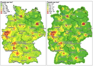
Figure 4 shows a comparison between population density and tweet density for the filtered tweets in the study region of Germany. The patterns are clearly broadly similar for both variables. This is confirmed by the correlation coefficient (Pearson) of 0.94. The highest densities in both estimations are in Berlin, in the Rhine-area, in Hamburg and in Munich. This also confirms an earlier statement that “where there is electricity [people], there are tweets [41].” For the tweet density estimation there is a considerable higher con-centration in metropolitan areas, which may be explained by the fact that there is a higher proportion of young people in these regions. Hence, there is also a proportion of people that has a high affinity to use mobile devices and services such as Twitter.
Figure 3: Representation of the relative proportions of the different attributes used for the filtering of raw data.
3.3
Points of interest
Points of interestare point-shaped objects that have a distinct meaning in the use of maps and navigation systems depending on the scope of the map or the navigation system [66]. These may be objects such as shops, restaurants, hospitals, or touristic attractions. Objects that are particularly prominent are also termed landmarks [60]. Within our model, we use classified points of interest (POI) to simulate the context of the proximity of each tweet, extracting POI data from OpenStreetMap (OSM).
Figure 4: Comparison of population density and tweet density in Germany. Left: pop-ulation density (~80.5m people), right: tweet density on mobile devices with German as detected language (period 9/2012–4/2013, ~500k tweets, cf. Figure 3). Both visualizations are based on kernel density estimation (KDE) using a Gaussian kernel with radius of 25km. Pearsons’ correlation coefficient between both KDEs isr= 0.94.
using their centroid. Data inconsistencies are part of the nature of the OSM project, as the classification of POIs in OpenStreetMap is collaborative process. Although there are map-ping guidelines documented in the Wiki of the project [50], their interpretation remains a subjective process. On some occasions there is even a lack of consistent mapping con-ventions. However, we assume that these inconsistencies are not of high relevance for our work, since we focus on relatively unambiguous POI feature classes.
4
Methods and results
As we explained in the introduction to this paper, our aim is to explore the extent to which georeferenced micro-blogging content can be related to its location. In order to analyze the potential link between tweets and location, we need a model for spatial context. One solution is using a set of classified points of interest as representative of some form of spatial context. Hence, the question of correlation between location and content can be reformulated as are the contents of the tweets related to nearby POI feature classes?
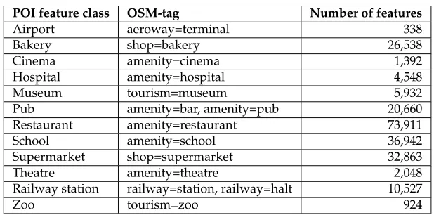
POI feature class OSM-tag Number of features
Airport aeroway=terminal 338
Bakery shop=bakery 26,538
Cinema amenity=cinema 1,392
Hospital amenity=hospital 4,548
Museum tourism=museum 5,932
Pub amenity=bar, amenity=pub 20,660
Restaurant amenity=restaurant 73,911
School amenity=school 36,942
Supermarket shop=supermarket 32,863
Theatre amenity=theatre 2,048
Railway station railway=station, railway=halt 10,527
Zoo tourism=zoo 924
Table 1: POI feature class, corresponding OSM-tag and number of features in the study region of Germany extracted from the OSM-dump (date of dump: 23/10/2013).
classification, supervised machine classification using manual training data and unsuper-vised machine classification using lexical training data.
4.1
Classification of microblogging texts
4.1.1 Manual classification
Methods The manual classification is the simplest, but most time consuming and least
scalable, approach from a methodological point of view. Each text is classified by one or more so-called humanannotators. The only classification rule that they are given is to evaluate, whether a text is related to a specific POI feature class. A classification by multiple annotators reduces the effect of subjective ratings. An uneven number of annotators is advantageous, as then for each text classification a majority judgment is possible. The set of all classified texts may subsequently be used as input for supervised machine learning. In information science this is also called agold standard[70].
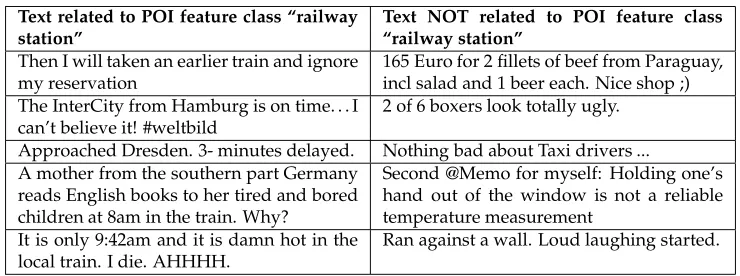
Here, we use the following geographically specific feature classes “railway station,” “cinema,” “restaurant,” and “supermarket,” whose relatedness to 5,000 randomly selected tweets was evaluated by three human annotators. 2,500 of the 5,000 tweets were selected considering the constraint that they should not be more than 250m away from the nearest instance of the respective POI feature class. This allows us to directly analyze whether the proportion of related tweets is higher in the set of “near tweets” than in the set of “random tweets,” where distance to POIs was not used as a selection criterion. Furthermore, as we initially assume a location-content correlation, a high proportion of related tweets in the set of “near tweets” would generate more training samples for the supervised machine learning. In order to illustrate the approach, Table 2 contains five examples of tweets that have consistently been evaluated as being (not) related to the POI feature class “railway station.”
Text related to POI feature class “railway station”
Text NOT related to POI feature class “railway station”
Then I will taken an earlier train and ignore my reservation
165 Euro for 2 fillets of beef from Paraguay, incl salad and 1 beer each. Nice shop ;) The InterCity from Hamburg is on time. . . I
can’t believe it! #weltbild
2 of 6 boxers look totally ugly.
Approached Dresden. 3- minutes delayed. Nothing bad about Taxi drivers ... A mother from the southern part Germany
reads English books to her tired and bored children at 8am in the train. Why?
Second @Memo for myself: Holding one’s hand out of the window is not a reliable temperature measurement
It is only 9:42am and it is damn hot in the local train. I die. AHHHH.
Ran against a wall. Loud laughing started.
Table 2: Five example texts that have consistently been evaluated as (not) being related to the POI feature class “railway station” (translated from German).
generalization of Fleiss’ Kappa [22] for the case of multiple annotators proposed by Con-ger [14].
The feature class “railway station” serves as first study example. The results showed that annotators predominantly judged microblogging texts to be relevant to this feature class that are in the widest sense about the topic “public transport,” e.g., texts about de-layed, crowded, or messy trains; the departure or arrival in a city; unusual events in trains or at railway stations; as well as texts about having just caught or missed a train. Ta-ble 3 shows a detailed IAA-analysis for this classification. According to the interpretation scheme of Fleiss’ Kappa proposed by Landis et al. [39], the IAA of the set “near tweets” are in “almost perfect” agreement, while the IAA of the set “random tweets” are in “substantial agreement.” The slightly better agreement for the set “near tweets” may be a result of the higher number of relevant tweets in this set, which enabled the annotators to evolve their decision criteria more precisely.
Set “near tweets”(distance tweet–POI<250m), overall agreement=0.81
Annotator 2 Annotator 3 Gold standard
Annotator 1 0.77 0.88 0.94
Annotator 2 0.79 0.84
Annotator 3 0.95
Set “random tweets” (arbitrary distance tweet–POI), overall agreement=0.72
Annotator 2 Annotator 3 Gold standard
Annotator 1 0.78 0.73 0.94
Annotator 2 0.65 0.84
Annotator 3 0.8
Table 3: Detailed IAA-analysis of the annotation of tweets according to their relevance to the POI feature class “railway station.” The column “gold standard” contains the majority votes of all annotators.
POI feature class IAA (mean of set “near” and set “random”)
Railway station 0.75 (substantial)
Cinema 0.63 (substantial)
Restaurant 0.48 (moderate)
Supermarket 0.54 (moderate)
Table 4: IAA of the relevance judgment of tweets to different POI feature classes.
for the feature class “railway station,” with the least agreement being found for “restau-rant,” and “supermarket.”
Table 5 shows the proportions of the relevant tweets with respect to the distance class of the nearest object of the corresponding feature class. It can be seen that there is a strong dependency in the proportion of relevant tweets from the distance to the nearest objects of the feature class “railway station.” Near to railway station, i.e., tweets that are closer than 250m to the nearest centroid of a railway station, the proportion of relevant tweets is about 10%, whereas for tweets that are further than 250m from the closest railway station object the proportion of relevant tweets is only 2%. For the other investigated feature classes the dependency of the proportion of relevant tweets from the distance is less significant. For the feature classes “cinema” and “supermarket” there is a decrease of 50% of the proportion of relevant tweets between near and distant tweets. For the feature class “restaurant” no meaningful difference in the proportion of relevant tweets may be observed.
A possible reason for that may be the selected distance threshold. As cinemas, restau-rants, and supermarkets are usually smaller than railway stations, their zone of influence may also be smaller. Thus, in Section 4.2 we describe a method which aims to derive a continuous analysis of distance dependency between content and POIs.
POI feature class Distance tweet–POI<250m Distance tweet–POI>250m
Railway station 246/2,500 (9.8%) 49/2,187 (2.2%)
Cinema 51/2,500 (2.0%) 24/2,335 (1.0%)
Restaurant 60/2,500 (2.4%) 33/1,462 (2.3%)
Supermarket 30/2,500 (1.2%) 7/1,754 (0.4%)
Table 5: Portion of tweets that are related to different POI feature classes.
4.1.2 Supervised machine classification using manually classified training data
Manual classification is a time- and resource-intensive process and thus, automation is de-sirable. This would support investigating a larger sets of tweets with respect to the location-content correlation. As introduced in Section 2.3, such automation may be achieved through supervised machine classification.
In previous research work, a method that is similar to ours has been used for the clas-sification of situational awareness [64] during mass emergencies where training data was manually annotated with respect to the relevance of individual tweets to events.
cases—but not in all cases—of text classification [49]. As the performance of a classifica-tion algorithm depends on the classificaclassifica-tion scenario, a comparison of both algorithms is recommended and was undertaken in our work.
Pre-processing of microblogging texts The frequent occurrences of (internet) slang,
ab-breviations, and misspellings make the automatic text classification more challenging. In order to overcome these problems, we pre-processed the texts. First, we removed URLs, punctuation, special characters, and emoticons. Subsequently, we standardized terms by lemmatization [27] and stemming [11, 18] and remove very common so-called stop words which do not contribute to class disambiguation.
Methods for the evaluation of the results In order to evaluate the results of the
super-vised machine classification, we used the confusion matrix shown in Figure 5. From this scheme four classic evaluation criteria from information retrieval can be derived:precision, recall, F-measure, andaccuracy.
Figure 5: Confusion matrix for supervised machine classification (adaption of [7]).
The precision (P) of the machine classification denotes the ratio of correctly classified documents to all classified documents (tweets in our case). High precision implies that many documents that have been found are actually relevant for a specific class.
P = rp
Recall(R)describes the ratio of all correctly classified documents to all relevant documents. High recall implies that most of the relevant documents were found by the machine classi-fication, while a low recall indicates that many relevant documents were not identified.
R=r rp
p+fn (2)
The F-measure(F)is the harmonic mean of precision and recall. As machine classification may either be optimized for good precision or for good recall, this measure may be used to find an optimal solution for both criteria.
R=P2P R+R (3)
Accuracy(A)describes the ratio of all correct classifications to all wrong classifications, by contrast to the previous measures, across all possible classes.
A= rp+rn
fp+fn (4)
Tuning of the classifier The result of the supervised machine classification for each
docu-ment is a probability value for each possible class, where the sum of all probabilities is 1. In the case of two possible classes, the default threshold that distinguishes both classes is 0.5. By using manual classified test data the optimum threshold with regard to the F-measure can be identified.
Results In order to compare the performance of NB and ME, we used the set of tweets that
were manually classified regarding their relatedness to the feature class “railway station.” The set of “near tweets” serves as training data and the set of “random tweets” serves as test data. Using different sets for training and testing a classifier may lead to slight underestimation of the classification performance. However, using both sets for training and testing ensures that all manually classified tweets are employed. Moreover, we do not expect related topics to be significantly different in both sets. Table 6 shows the confusion matrices for both algorithms.
a) Confusion matrix, algorithm=ME, row=true, column=predicted, accuracy=0.98
Label Yes No Total Precision Recall F-measure
Yes 44 39 83 0.95 0.53 0.68
No 2 2415 2417 0.98 1.00 0.99
b) Confusion matrix, algorithm=NB, row=true, column=predicted, accuracy=0.96
label Yes No Total Precision Recall F-measure
Yes 26 57 83 0.84 0.32 0.46
No 5 2412 2417 0.98 1.00 0.99
It may be seen that ME reaches both higher precision (0.95 versus 0.84) and also higher recall (0.53 versus 0.32). A comparison of the F-measures using classified tweets of all four manually annotated feature classes as training and test data confirms the better perfor-mance of ME for this classification task (Table 7). In what follows, we therefore restrict ourselves to the use of ME in the classification task.
POI feature class F-measure ME F-measure NB
Railway station 0.68 0.46
Cinema 0.26 0.00
Restaurant 0.29 0.07
Supermarket 0.18 0.10
Table 7: Comparison of the performance of ME and NB classification using the F-measures for feature class identification.
0 50 100 150 200 250
0.0
0.2
0.4
0.6
0.8
1.0
number of training documents
F
−
measure
, precision, recall
F−measure precision recall railway station cinema restaurant supermarket
Figure 6: Correlation of the performance of supervised machine classification and the number of training documents. Classification method: ME.
The example of the feature class “railway station” allows us to investigate the rela-tionship between the number of relevant training documents and the classification perfor-mance expressed by precision, recall and F-measure. For this purpose, some of the man-ually classified documents were removed from the training process. Figure 6 shows that at least 100 training texts are needed to reach a performance of F-measure>0.5. It may be seen that a further increase of the number of training documents also results in a better classification performance. However, above approximately 200 training texts the rate of performance improvement reached by using more documents for training gets lower.
Related to railway station Not related to railway station
German stem English Weight German stem English Weight
bahn railway 2.64 sag say 0.53
zug train 2.30 schlaf sleep 0.47
sbahn urban railway 2.12 uberhor miss 0.47
ubahn subway 2.03 viel much/many 0.46
bus bus 1.99 abraum clear 0.46
hbf main station 1.85 toast toast 0.46
bahnhof railway station 1.74 wer who 0.40
hauptbahnhof main station 1.71 abend evening/night 0.39
ice high-speed train 1.50 trink drink 0.36
aussteig exit 1.43 lieb love 0.35
verspatung delay 1.20 seh see 0.34
u subway 1.06 letzt last 0.33
db deutsche bahn 0.99 glaub believe 0.32
station station 0.98 ja yes 0.30
braunschweig braunschweig 0.95 besuch visit 0.30
busfahr go by bus 0.95 freu be happy 0.29
sitz sit/seat 0.94 nein no 0.29
ic intercity train 0.90 vielleicht maybe 0.29
bvg Bvg 0.84 allein lonely 0.29
dresd dresden 0.83 spiel play/match 0.29
berlin berlin 0.82 auskost savour 0.28
erreich arrive 0.80 auto car 0.27
schienenersatzverkehr rail replacement 0.75 such look for 0.27
Table 8: Top 20 features for the class “related to railway station” and the class “not related to railway station.” The weights are determined by ME using manually classified training data. German words are stems, English words are translations (not stemmed).
tweets”). The high weights of the toponyms “Braunschweig,” “Berlin,” and “Dresden” are due the coincidence that each of them occurs in three texts that have been classified as being relevant to the POI feature class “railway station,” usually in the context of arriving in or departing from the corresponding city. As these toponyms did not occur in texts that were not relevant, they seem to be significant for the feature class railway station from the perspective of the ME algorithm. Furthermore the weights of both feature vectors show that indeed there are highly significant words that indicate relevance to railway station objects, whereas there is no word that equally significantly indicates that a certain text is not relevant to railway station objects.
POI feature class Distance tweet–POI
<250m
Distance tweet–POI
>250m All tweets
Railway station 697/10,958 (6.4%) 1,263/89,042 (1.4%) 1,960/100,000 (2.0%)
Cinema 23/5,390 (0.4%) 70/94,610 (0.1%) 93/100,000 (0.1%)
Restaurant 62/39,971 (0.2%) 105/60,029 (0.2%) 167/100,000 (0.2%)
Supermarket 11/28,443 (0.04%) 16/71,557 (0.02%) 27/100,000 (0.03%)
Table 9: Portion of tweets that are related to different POI feature classes.
Manually annotated tweets: related to railway station (yes/no)
Distance tweet − nearest railway station object (m)
Density
10 50 500 5000 50000
yes max= 191 m median= 328 m no max= 428 m median= 931 m
Machine annotated tweets: related to railway station (yes/no)
Distance tweet − nearest railway station object (m)
Density
10 50 500 5000 50000
yes max= 172 m median= 448 m no max= 378 m median= 1003 m
Figure 7: Density plots of the distributions of tweets with regard to their distance to the nearest railway station on logarithmic scale. Left: results of manual classification, right: results of machine classification.
The main reason for that is the low quantity of training documents for these feature classes—51 for “cinema,” 60 for “restaurant,” and 30 for “supermarket” in contrast to 246 for “railway station” (Table 5), which results in a lower performance of the supervised machine classification (Figure 6). However, for the POI feature classes “railway station,” and “cinema” the dependency of the proportion of relevant tweets from the distance to the nearest instances that has been shown with manual classification (Table 5) is also confirmed by the results of the machine classification.
4.1.3 Unsupervised machine classification using lexical training data
As the creation of manual training data is a time-consuming process, we sought for an un-supervised method not dependent on manual training data. This would allow us to easily investigate further POI feature classes with regard to their location-content correlation.
Methods A possible approach is to derive words that are relevant to a certain POI feature
class using an existing corpus. In this approach, the significance of sentence co-occurrence could be used to identify relevant words. A similar approach has shown that it is possible to derive overall movie ratings, by analyzing the significance of the co-occurrence of all uni-and bigrams co-occurring in a movie review with the words “excellent” uni-and “poor” [63]. For the work presented in this paper, the names of the POI feature classes are used as entry point to derive co-occurring words. We assume that terms related to our POIs (in German), such as “railway station,” “restaurant,” “cinema,” or “supermarket,” may be interpreted as category nouns.
TheWortschatz project [24, 53] is a candidate corpus containing pre-processed signif-icance scores for co-occurring words. The news corpus was compiled by automatically crawling news websites and since Wortschatz corpora are available in many languages, the approach may be implemented in languages other than German. We used the corpus “2010-news-10M” which contains 10M sentences [28]. It has already been shown that there is a significant overlap between topics discussed in Twitter and topics discussed in news media [72], though the bias in Twitter towards personal life, pop culture, and celebrities needs to be acknowledged.
The significance scores were computed by Biemann et al.’s [6] adaption of the log-likelihood-measure described by Dunning [21]. We used these significance scores to derive pseudo-texts specific for each POI feature class that we want to investigate. Each of these pseudo-texts consists of 40,000 sentences, of which 20,000 belong to the class “relevant to this POI feature class.” Each sentence consists of 10 words. The probability that a specific word is selected for such a sentence is shown in (5), where swi denotes the score of the
significance of the co-occurrence of a specific word with the name of the POI feature class. The name of the POI feature class is selected as a word with the same probabilitypmax(w) as the most significant co-occurring word.
p(wi) =is=wni
i=1swi
(5)
The remaining 20,000 sentences belong to the class “not relevant to this POI feature class.” Likewise, each of these sentences consists of 10 words. For these words the prob-ability of a specific word (6) is defined by the frequency of this word fwi in the whole
Wortschatz corpus.
p(wi) = if=wni
i=1fwi
(6)
Results Table 10 shows the top 20 co-occurring words for the word “Bahnhof” (English: “railway station”), their frequencies in the whole corpus, their co-occurrence frequency and the co-occurrence significance scores. It can be seen that there is a significant overlap with the words contained in the model generated from the manually classified texts, e.g., train/trains, railway, track/tracks, main station, urban railway, Inter City etc. (cf. Table 8). This can be interpreted as an indication of the suitability of this corpus as a substitute to manually classified training data.
Finally, Table 11 confirms a partial overlap between the feature vectors of the classifi-cation model derived from the manually classified documents and the classificlassifi-cation model derived from lexical data (cf. Table 8), e.g.: railway station, train, track, railway, inter city express, urban railway and main station.
Word Translation Word frequency Co-occurrence
frequency
Co-occurrence significance
Am at 668,908 1,903 3,644
Zug train 8,277 272 1,700
Uhr clock 139,603 496 1,077
zum to 405,093 722 719
Richtung direction 31,723 207 642
Bahn railway 16,594 163 632
vom from 193,066 455 624
dem the 1,038,370 1,176 582
Gleise tracks 1,086 67 498
Z ¨uge trains 4,184 85 444
Am At 103,759 260 368
Gleis track 662 46 355
Stuttgart Stuttgart 25,495 128 344
Hauptbahnhof main station 2,465 59 327
Zoo zoo 1,897 54 319
Bundespolizei police 2,552 58 316
Altona Altona 332 36 311
Stuttgarter Stuttgart’s 7,559 79 310
Stadt town 68,084 186 291
fahren go 17,804 100 277
S-Bahn urban railway 1,767 45 271
ICE Inter City Exp. 1,515 45 270
den the 1,954,007 1,508 264
unterirdischen below ground 713 36 252
Table 10: Co-occurring words and corresponding frequencies and significance-scores for the word “Bahnhof” (engl.: “railway station,” word frequency=5,925) taken from the “2010 news 10M sentences” corpus of the Wortschatz project.
Related to railway station Not related to railway station
German stem English Weight German stem English Weight
bahnhof railway station 2.30 dass that 0.90
zug train 1.94 muss must 0.79
gleis track 1.87 jahr year 0.78
bahn railway 1.58 sag say 0.74
unterirdisch subsurface 1.49 geb give 0.72
bundespolizei police 1.45 erst only 0.66
ice inter city expr. 1.44 prozent percent 0.66
richtung direction 1.41 gut good 0.64
Stuttgart Stuttgart 1.39 euro euro 0.63
Neustadt Neustadt 1.39 spiel match 0.62
sbb swiss railway 1.38 deutsch German 0.62
sbahn urban railway 1.37 geh go 0.60
reisend traveller 1.34 seit since 0.58
treffpunkt meeting point 1.34 schon already 0.54
Fischbach Fischbach 1.34 ganz all 0.53
hauptbahnhof main station 1.34 viel many 0.53
Altona Altona 1.34 bleib stay 0.52
bahnsteig platform 1.33 imm always 0.52
fahrgast passenger 1.31 ebenfall likewise 0.52
Harburg harburg 1.29 weit far 0.50
Stadelhof Stadelhof 1.27 durf may 0.50
schnellzug express train 1.26 million million 0.49
sonderzug special train 1.25 tag day 0.49
zoo zoo 1.25 Deutschland Germany 0.47
Castelldefel Castelldefel 1.25 lieg lie 0.47
Table 11: Top 20 features for the class “related to railway station” and the class “not related to railway station.” The weights are determined by ME using lexical training data. German words are stems, English words are translations (not stemmed).
the unsupervised machine classification using lexical training data does not reach the same classification performance as the classification using manually classified training data.
However, the unsupervised machine classification using lexical training data does out-perform a random baseline model and an inverse distance weighted baseline model. Thus, we can conclude that a significant signal may be detected by this approach, as is confirmed by a comparison of the F-measures shown in Table 13.
a) Confusion matrix, algorithm = ME, row=true, column=predicted, accuracy=0.98, training data = lexical
Label Yes No Total Precision Recall F-measure
Yes 28 55 83 0.82 0.33 0.47
No 6 2411 2417 0.98 1 0.99
b) Confusion matrix, row=true, column=predicted, accuracy=0.94, training data = random weights
Label Yes No Total Precision Recall F-measure
Yes 4 79 83 0.07 0.05 0.06
No 71 2346 2417 0.97 0.97 0.97
c) Confusion matrix, row=true, column=predicted, daccuracy=0.95, training data = inverse distance weighted
Label Yes No Total Precision Recall F-measure
Yes 17 66 83 0.25 0.21 0.23
No 50 2367 2417 0.97 0.98 0.98
Table 12: Comparison of the classification performance (F-measure) for railway station based on (a) lexical training data, (b) a random model and (c) an inverse distance weighted model.
Manually classified training data
Lexical training data
Inverse distance baseline
Random baseline
Railway station 0.68 0.47 0.23 0.06
Cinema 0.45 0.31 0.02 0.04
Restaurant 0.40 0.33 0.09 0.02
Supermarket 0.25 0.17 0.02 0.00
Table 13: Comparison of the F-measures for the POI-feature classes, for which manually classified test data exists.
4.2
Computation of the distance dependency
4.2.1 Method
Assuming that all tweets have been classified regarding their relatedness to the respective feature classes, the dependency of the proportion of the related tweets from the distance to the closest POI instance of that feature class may be computed as follows. For this purpose, all POI features are modeled as points (Figure 9) and each tweet is attributed to the closest POI instance of the respective class.
0.0 0.2 0.4 0.6 0.8 1.0
0.0
0.2
0.4
0.6
0.8
1.0
precision
recall
railway station cinema restaurant supermarket
Figure 8: Relationship of precision and recall for the automatic classification using lexical training data while tuning the classification threshold.
1 2 3 4 5
Figure 9: Computation of the proportion of related tweets with regard to the distance to the closest POI-feature. Blue dots: POIs (3), red dots: related tweets (6), grey dots: unrelated tweets (24).
4.2.2 Results
related tweets within a distance of 50m is about 7 times higher than the average (~25% versus 3.3%). For the feature classes “restaurant” (~5% versus 2.2%), and the feature class “supermarket” (~1.8% versus 0.6%) the proportion within a distance of 50m is only 3 times above average. For the feature class “cinema,” no distance dependency was observed. This contradicts the results found by manual classification (Table 5) and may be explained by an anomaly in the comparably small test data set.
Moreover, Figure 10 confirms the assumption that the different POI feature classes, which differ in their extent and their importance, have varying zones of influence. The threshold of 250m, selected in Table 5 is too high to observe a distance dependency in the proportion of related tweets for the feature classes “cinema,” “restaurant,” and “supermar-ket.”
50 100 200 500 1000 2000 5000 10000 20000 50000
0.5
1.0
2.0
5.0
10.0
20.0
distance Tweet − nearest POI−object (m)
share of T
w
eets related to the respectiv
e POI
−
feature class (%)
railway station (mean=3.3%, 83 classified docs) cinema (mean=1.0%, 25 classified docs) restaurant (mean=2.2%, 56 classified docs) supermarket (mean=0.6%, 14 classified docs)
Figure 10: Dependency of the proportion of texts that are related to a specific POI-feature class on the distance between the position of text creation and the nearest POI-feature. The results are derived from the manually classified documents. The horizontal lines denote the proportion of tweets related to this POI-feature class in the whole corpus.
some of the feature classes—e.g., “airport” and “railway station”—there is a clear distance dependency in the proportion of related tweets. However, for some other feature classes no such dependency is visible.
50 100 200 500 1000 2000 5000 10000 20000 50000
0.02
0.05
0.10
0.20
0.50
1.00
2.00
5.00
10.00
20.00
distance − nearest POI−object (m)
share of T
w
eets related to the respectiv
e POI
−
feature class (%)
railway station (mean=1.78%) airport (mean=0.29%) cinema (mean=0.87%) theatre (mean=0.39%) restaurant (mean=1.14%) bar/pub (mean=0.14%) supermarkt (mean=0.66%) bakery (mean=0.02%) zoo (mean=0.09%) museum (mean=0.24%) school (mean=0.32%) hospital (0.21%)
Figure 11: Dependency of the proportion of texts that are related to a specific POI-feature class from the distance between the position of text creation and the nearest POI-feature. The results are derived from the unsupervised classified documents using lexical training data. The horizontal lines denote the proportion of tweets related to this POI-feature class in the whole corpus.
A comparison of the results with those reached using manually classified data shows that the patterns for “railway station,” “restaurant,” and “supermarket” are qualitatively similar. However, there are significant quantitative differences, which may be explained by the low recall of the automatic classification approach (cf. Section5.3). Further features classes that show a clear distance dependency in their proportion of related tweets are “zoo,” “hospital,” and “theatre.” For “bakery,” “bar/pub,” “museum,” and “school” there is no clear distant-dependent trend.
Finally, Figure 12 shows the probability density function of related tweets for multiple POI-feature classes based on lexical training data. From this analysis, it may be concluded that 50% of all tweets detected as being related to railway station are within 500m of the nearest railway station. This finding could help improving automatic georeferencing of tweets, as in turn it may also be inferred that a tweet that has been automatically classi-fied as being related to a railway station has a 50% probability of being within 500m of the nearest railway station object (in Germany). However, it should also be noted that also 30% of the tweets that are explicitly not related to a railway station are also within 500m of the nearest railway station. This simply illustrates that many tweets are located in city centers, where both railway stations and “tweeting people” are typically found. A similar trend is also found for airport features, with the key difference that a much smaller proportion of all tweets not related to airports are found nearby, once again illustrating the peripheral posi-tioning of airports. For the other classes graphed (cinema, supermarket, and hospital), the two curves are almost identical, confirming the lack of specificity of distance in explaining the locations where individuals tweeted on these themes.
50 100 200 500 1000 2000 5000 20000 50000
0
2
04
06
08
0
1
0
0
distance Tweets − nearest POI−Object (m)
share of related / non
−
related T
w
eets (%)
related to railway station non−related to railway station related to cinema
non−related to cinema related to supermarket non−related to supermarket related to airport non−related to airport related to hospital non−related to hospital
5
Interpretation
5.1
Manual classification
The two main problems with the manual classification are costs and subjectivity of the classification. While the first problem results from the overall low proportion of relevant texts and the resulting large number of texts that must to be classified in order to create an adequate sample, the latter problem is intrinsic to this classification method. Subjectivity may partially be overcome by the classification of the texts by multiple annotators. The subjectivity of the classification is potentially increased by the necessarily general classifi-cation guidelines, where annotators were only asked whether a specific text was related to a specific POI-feature class. The lack of context due to the character limit of Twitter mi-croblogging texts (140) made the task even more challenging and the classification prone to disagreement.
However, the results for the inter-annotator-agreement (Table 4) lay between 0.75 (“sub-stantial agreement”) and 0.48 (“moderate agreement”). This demonstrated that classifica-tion was strongly dependent on POI feature class, but nonetheless reasonable results were achievable. One potential reason for these differences depending on the feature class may be that the names of the feature class do not serve as category nouns in all cases. For ex-ample, many German speakers would prefer to say “going to/being at ALDI” over “going to/being at the supermarket,” which has implications for associations with the POI-feature class name.
Furthermore, some of the POI-feature classes may be more ambiguous than others. For example, “food” may be a topic that is related to the feature class “restaurant.” However, for an annotator it may not be clear, whether a text about food relates to a restaurant or some other location.
5.2
Supervised machine classification
The main benefit of this approach is that an arbitrary number of texts may be rapidly classi-fied with some known classification quality so long as training and testing data is available. For the POI-feature class “railway station” a good classification performance was achieved (precision=0.95, recall=0.53, F-measure=0.68, cf. Table 6). However, for the other tested feature classes the results were less convincing (cf. Table 7). One key reason for this poor performance is likely to be the lower numbers of training samples for these feature classes. While for the class “railway station,” we worked with 246 manually classified texts, for “cinema” (51), “restaurant” (60), and “supermarket” (30) significantly fewer sam-ples were identified during the manual classification task, which also suggests a lower proportion of tweets related to these feature classes in the whole corpus. Our sensitivity tests indicated that least 100 samples are needed in order to reach a good classification performance (i.e., F-measure>0.5, cf. Figure 6). One approach to increasing the sample size would be simply to build a larger training data set, for example by using crowd sourcing in the classification task (cf. [9, 20, 36]).
Fur-thermore, the complexity of NLP caused by the use of slang may only partially resolved by the applied techniques lemmatization and stemming.
With regard to the analysis of the location-content correlation, the results of this classi-fication method lead to similar conclusions if enough training data is available (cf. Table 5, Table 9).
5.3
Unsupervised machine classification
The main benefit of this classification approach is that the costly training data generation process is not necessary. The analysis of the significance of the co-occurring words in the applied corpus “Wortschatz news” showed a partial overlap with the classification model derived from manual classification (Table 8, Table 10, Table 11). However, the substitution of manual training data by lexical training data leads to a loss of 33% of classification per-formance. Likewise, in comparison with the human classification the poor performance is obvious (average F-measure of only 0.32, Table 13).
However, it could also be shown unsupervised machine classification outperformed random and inverse distance weighted baselines, suggesting that this approach does in-deed have potential. Its advantage is that it is independent from the subjectivity of indi-vidual annotators and of course reduces the need for costly training data.
Method Costs Degree of automation Classification quality
Manual classification high no automation high
Supervised machine classification high medium medium
Unsupervised machine classification low high low
Table 14: Schematic comparison of the three classification methods.
5.4
Distance dependency of the proportion of related tweets
The patterns of the distance dependency of the proportion of the tweets being related to nearby POI instances are, in the main, qualitatively similar when we compare manual and machine classification (Figure 10, 11). However, the patterns differ quantitatively, which can be explained by the low recall of the machine classification approaches. Differences in the distance patterns between the different investigated feature classes may on the one hand be explained by the different arrangement of the feature instances in space and on the other hand by the extent to which users are stimulated to write about these feature classes when being in their locale.
In interpreting the results it is important to note that we did not consider temporal usage patterns. Potentially, if data was filtered for peak usage times of individual feature classes, then distance dependencies might increase.
5.5
Points of interest as a model for geospatial context
presumably lower than it would be if tweets created near to railway lines were also con-sidered as near tweets by the chosen model. Beside the geometric simplification—points only—the model also contains a semantic simplification of the reality. At many locations not only the classified POIs contained in the applied model serve as a stimuli for writing spatially influenced tweets, but also other objects not contained in the model. Thus, other models for the geospatial context might lead to different results of the location-content cor-relation of tweets. For instance, a higher location-content corcor-relation might be expected for topographic objects with proper names, such as the Eiffel Tower, the Brandenburg Gate, or individual outlets of McDonald’s.
6
Concluding discussion
6.1
Recalling the research questions
(1) How can we represent spatial context in order to investigate the relationship between the information content and its surroundings?
For our approach we used a set of classified points of interest to represent spatial context. The advantage of this approach is that such a set is easily available and the analysis is simple. The disadvantage is however that geometry and semantics are highly abstracted. In contrast to previous research that used toponyms [12, 29, 67] as well as highly specific regions of interest [2], POIs allow us to model spatial context at high resolutions.
(2) How can individual texts be classified such that content can be related to surround-ings?
We explored three options for this classification task: manual classification by human an-notators, supervised machine classification using training data generated by human anno-tation and unsupervised machine classification using training data that is derived from an existing corpus. The main challenge for all three approaches is that microblogging texts are very short and thus contextual information is sparse. However, all three methods tested have strengths and weaknesses, with the important caveat that a larger testing dataset is essential given the low sample sizes of relevant texts in some classes.
(3) Can we automate this classification process by means of machine learning?
(4) Which learning algorithms would be best suited for such kind of automation?
Previous research has suggested the algorithms naive Bayes, maximum entropy, and sup-port vector machines [51,64]. We tested NB and ME as they are implemented in the applied software Mallet [45] finding that ME outperforms NB by 50% on average (cf. Table 7) for the tested feature classes.
(5) Is there a corpus that allows us to appropriately substitute manual training data for the classification task?
Previous work pointed to a thematic overlap between topics discussed on Twitter and top-ics presented on news websites [72]. This suggests using a corpus generated from news websites to derive training data that may substitute manual training data. We therefore used the corpus “Wortschatz news” and selected words that significantly co-occur with the titles of POI-features as models to find texts related to these feature classes. The results show that the machine classification using this substitution performs some 30% worse than the machine classification using manually classified training sample (cf. Table 13). How-ever, the results regarding the location-content correlation of the tweets using this substi-tution are qualitatively similar for 3 of the 4 tested feature classes (Figure 10, 11). This indicates that if precision can be maintained, even at the cost of low recall, it is still possible to extract meaningful relationships between POIs and the locations of individual tweets.
(6) Does the proportion of texts related to location-specific information show a decay over distance—in other words are the locations of the texts which relate to specific loca-tions non-randomly distributed in space?
Our analysis of location-content correlation using the model of the relevance of the texts for selected POI-feature classes does not yield homogeneous results. For some feature classes a significant distance dependency of the proportion of related tweets may be determined. For these feature classes it may be concluded that related tweets are not completely randomly distributed in space. For instance, for the feature class “railway station,” at a distance of 100m, about 8–20% of tweets are related to the feature class, a significantly higher propor-tion than the 2–3% of tweets in the corpus as a whole related to the class.
Nevertheless, the general conclusion that the current location of the users does not dom-inate their microblogging-activities is consistent with their intentions [17, 32] of using the service, which are in the main daily chatter and personal communication. Both activities do not necessarily need to be influenced by the spatial context.
In order to maintain consistency with prior research it is important to mention that the intensity of the location-content correlation also seems to depend on the scale of the analysis. Such a correlation would be consistent with previous findings [2, 12, 29, 30, 56, 67], which demonstrated a location-content correlation at small and medium cartographic scales.
Last but not least, location-content correlation is also likely to depend on the temporal dimension, as topics which are relevant in social networks seem to depend on time [69]. We assume that location-content correlation would be higher, if we consider temporal patterns. However, we have not tested this in the current research work.
6.2
Implications of the findings
The findings regarding the low correlation between location and content of mobile gen-erated microblogging texts on high resolution have implications for the automatic geo-referencing of microblogging texts for large cartographic scales. The potential increase of the accuracy of the geo-referencing by using their spatial correlation to classified points of interest is limited and depends on the specific POI-feature class. One possible approach to partially overcoming this limitation might be the analysis of the social network of a user including her/his conversation as well as her/his history of tweets. It seems reasonable to assume that such information might improve the accuracy of geo-referencing through tweet content, though we would emphasize that such a correlation remains speculation.
A more general conclusion is that the application of tweet-analyses for high resolution applications should be approached with care as the correlation between the contents and the locations of tweets that is required for these applications is probably often too low. Thus, applications that rely on the existence of a strong location-content correlation—such as (spatial) opinion-, emotion-, and sentiment-research, decision support systems for natu-ral hazards, or place descriptions—need to demonstrate whether geo-referenced tweets are suitable for the corresponding application. Crampton et al. [15] conclude in this context that the scale of analyses of tweets needs to be adapted to their spatial resolution. Fur-thermore, they emphasize that culture, religion, and language have an impact on spatial patterns of tweets. On the other hand, however, also long distances may be spanned by the ties in what is after all also a social network. Hence, the structure of these networks also needs to be understood in order to understand the spatial patterns of tweet distribution.
Furthermore, our findings suggest that for high resolution spatial analyses of tweets automatic filtering and validation methods are needed as essential. Given that work with Flickr and other photographically based social media seems to have demonstrated a more direct location-content correlation [16] we suggest that tweets containing photos could be preferably used in spatial analysis, particularly at large scales.
Acknowledgments
Research for this article is based upon work supported by the German Research Founda-tion (DFG, Deutsche Forschungsgemeinschaft) under the project “Mobile map applicaFounda-tions based on user generated content for cartographic communication” (BU 2605/1-1).
References
[1] AHERN, S., NAAMAN, M., NAIR, R., ANDYANG, J. H.-I. World explorer: Visualiz-ing aggregate data from unstructured text in geo-referenced collections. In Proc. 7th ACM/IEEE-CS Joint Conference on Digital Libraries (JCDL) (New York, NY and USA, 2007), ACM, pp. 1–10. doi:10.1145/1255175.1255177.
[2] ANDRIENKO, G., ANDRIENKO, N., BOSCH, H., ERTL, T., FUCHS, G., JANKOWSKI,
P., AND THOM, D. Thematic patterns in georeferenced tweets through
space-time visual analytics. Computing in Science and Engineering 15, 3 (2013), 72–82. doi:10.1109/MCSE.2013.70.
[3] ANDROUTSOPOULOS, I., KOUTSIAS, J., CHANDRINOS, K. V., AND SPYROPOULOS, C. D. An experimental comparison of naive Bayesian and keyword-based anti-spam filtering with personal e-mail messages. InProc 23rd Annual International ACM SIGIR Conference on Research and Development in Information Retrieval (SIGIR) (2000), ACM, pp. 160–167. doi:10.1145/345508.345569.
[4] ASUR, S., AND HUBERMAN, B. A. Predicting the future with social
me-dia. In Proc. IEEE.WIC.ACM International Conference on Web Intelligence and In-telligent Agent Technology (2010), N. Cercone, Ed., vol. 1, IEEE, pp. 492–499. doi:10.1109/WI-IAT.2010.63.
[5] BERGER, A. L., DELLAPIETRA, S., ANDDELLAPIETRA, V. J. A maximum entropy approach to natural language processing.Computational Linguistics 22, 1 (1996), 39–71. [6] BIEMANN, C., BORDAG, S., HEYER, G., QUASTHOFF, U.,ANDWOLFF, C.
Language-independent methods for compiling monolingual lexical data. InComputational Lin-guistics and Intelligent Text Processing, A. Gelbukh, Ed., vol. 2945 ofLecture Notes in Com-puter Science. Springer, Berlin, 2004, pp. 217–228. doi:10.1007/978-3-540-24630-5 27. [7] BIRD, S., KLEIN, E., AND LOPER, E. Natural language processing with Python, 1 ed.
O’Reilly, Cambridge, MA, 2009.
[8] BOLLEN, J., MAO, H.,ANDZENG, X. Twitter mood predicts the stock market.Journal of Computational Science 2, 1 (2011), 1–8. doi:10.1016/j.jocs.2010.12.007.
[9] CALLISON-BURCH, C., AND DREDZE, M. Creating speech and language data with amazon’s mechanical turk. InProc. NAACL HLT 2010 Workshop on Creating Speech and Language Data with Amazon’s Mechanical Turk (CSLDAMT)(2010), ACL, pp. 1–12. [10] CARSTENSEN, K.-U., EBERT, C., EBERT, C., JEKAT, S., KLABUNDE, R.,ANDLANGER,
[11] CAUMANNS, J.A fast and simple stemming algorithm for German words. PhD thesis, Freie Universit¨at, Berlin, 1999.
[12] CHENG, Z., CAVERLEE, J.,AND LEE, K. You are where you Tweet: A content-based
approach to geo-locating twitter users. InProc. 19th ACM International Conference on Information and Knowledge Management (CIKM)(2010), J. Huang, Ed., ACM, pp. 759– 768. doi:10.1145/1871437.1871535.
[13] CIULLA, F., MOCANU, D., BARONCHELLI, A., GONCALVES, B., PERRA, N., AND
VESPIGNANI, A. Beating the news using social media: The case study of American Idol. EPJ Data Science 1, 1 (2012), 8. doi:10.1140/epjds8.
[14] CONGER, A. J. Integration and generalization of kappas for multiple raters. Psycho-logical Bulletin 88, 2 (1980), 322–328. doi:10.1037/0033-2909.88.2.322.
[15] CRAMPTON, J. W., GRAHAM, M., POORTHUIS, A., SHELTON, T., STEPHENS, M., WILSON, M. W.,ANDZOOK, M. Beyond the geotag: Situating “big data” and lever-aging the potential of the geoweb.Cartography and Geographic Information Science 40, 2 (2013), 130–139. doi:10.1080/15230406.2013.777137.
[16] CRANDALL, D. J., BACKSTROM, L., HUTTENLOCHER, D.,ANDKLEINBERG, J.
Map-ping the World’s photos. InProc. 18th International Conference on World Wide Web(2009), J. Quemada and G. Le ´on, Eds., ACM, pp. 761–770. doi:10.1145/1526709.1526812.
[17] CRAWFORD, C. How informative is Twitter? http:blog.textwise.com/2010/01/08/
how-informative-is-twitter/, 2010. Accessed 04.01.2013.
[18] CRYSTAL, D. A Dictionary of Linguistics and Phonetics, 2nd ed. The Language Library. Blackwell, Oxford, 1985.
[19] DE LONGUEVILLE, B., SMITH, R. S., AND LURASCHI, G. “OMG, from here, I
can see the flames!”: A use case of mining location based social networks to ac-quire spatio-temporal data on forest fires. In Proc. 2009 International Workshop on Location Based Social Networks (LBSN) (2009), X. Zhou, Ed., ACM, pp. 73–80. doi:10.1145/1629890.1629907.
[20] DOWNS, J. S., HOLBROOK, M. B., SHENG, S.,ANDCRANOR, L. F. Are your partici-pants gaming the system? InProc. 28th SIGCHI Conference on Human Factors in Comput-ing Systems (CHI)(2010), E. Mynatt, D. Schoner, G. Fitzpatrick, S. Hudson, K. Edwards, and T. Rodden, Eds., pp. 2399–2402. doi:10.1145/1753326.1753688.
[21] DUNNING, T. Accurate methods for the statistics of surprise and coincidence. Compu-tational Linguistics 19, 1 (1993), 61–74.
[22] FLEISS, J. L. Measuring nominal scale agreement among many raters. Psychological Bulletin 76, 5 (1971), 378–382. doi:10.1037/h0031619.
[23] GAYO-AVELLO, D. No, you cannot predict elections with Twitter. IEEE Internet
Com-puting 16, 6 (2012), 91–94. doi:10.1109/MIC.2012.137.
[24] GELBUKH, A., Ed. Computational Linguistics and Intelligent Text Processing: Proceed-ings of 5th International Conference CICLing(Berlin and Heidelberg, 2004), vol. 2945 of
[25] GOODCHILD, M. F. Citizens as sensors: The world of volunteered geography. Geo-Journal 69, 4 (2007), 211–221. doi:10.1007/s10708-007-9111-y.
[26] GRAHAM, M., AND SHELTON, T. Geography and the future of big data, big data
and the future of geography. Dialogues in Human Geography 3, 3 (2013), 255–261. doi:10.1177/2043820613513121.
[27] HAMP, B., FELDWEG, H., ET AL. Germanet-a lexical-semantic net for German. In
Proc. ACL Workshop Automatic Information Extraction and Building of Lexical Semantic Resources for NLP Applications(1997), pp. 9–15.
[28] HAN, B.,ANDBALDWIN, T. Lexical normalisation of short text messages: Makn sens a #twitter. InProc. 49th Annual Meeting of the Association for Computational Linguistics: Human Language Technologies (HLT)(2011), vol. 1, ACL, pp. 368–378.
[29] HECHT, B., HONG, L., SUH, B., AND CHI, E. H. Tweets from Justin Bieber’s heart: The dynamics of the location field in user profiles. In Proc. SIGCHI Conference on Human Factors in Computing Systems (CHI) (2011), D. Tan, Ed., ACM, pp. 237–246. doi:10.1145/1978942.1978976.
[30] HERFORT, B., ALBUQUERQUE, J.D., SCHELHORN, S.-J.,ANDZIPF, A. Exploring the geographical relations between social media and flood phenomena to improve situa-tional awareness. InConnecting a Digital Europe Through Location and Place, J. Huerta, S. Schade, and C. Granell, Eds., Lecture Notes in Geoinformation and Cartography. Springer, Berlin, 2014, pp. 55–71. doi:10.1007/978-3-319-03611-3 4.
[31] HOLLENSTEIN, L.,ANDPURVES, R. E

![Figure 2: Schematic representation of supervised text classification using manually classi-fied training data (figure is an adaptation of Scharkows’ illustration [55]).](https://thumb-us.123doks.com/thumbv2/123dok_us/1157266.1617810/5.612.115.509.367.577/schematic-representation-supervised-classication-manually-adaptation-scharkows-illustration.webp)


![Figure 5: Confusion matrix for supervised machine classification (adaption of [7]).](https://thumb-us.123doks.com/thumbv2/123dok_us/1157266.1617810/13.612.133.492.320.581/figure-confusion-matrix-supervised-machine-classication-adaption.webp)