RESEARCHARTICLE
Evaluating existing manually
constructed natural landscape
classification with a machine
learning-based approach
Rok Cigliˇc
1, Erik Štrumbelj
2, Rok ˇ
Cešnovar
2, Mauro Hrvatin
1,
and Drago Perko
11Research Centre of the Slovenian Academy of Sciences and Arts, Ljubljana, Slovenia 2Faculty of Computer and Information Science, University of Ljubljana, Ljubljana, Slovenia
Received: September 4, 2018; returned: February 11, 2019; revised: March 27, 2019; accepted: May 16, 2019.
Abstract: Some landscape classifications officially determine financial obligations; thus, they must be objective and precise. We presume it is possible to quantitatively evaluate existing manually constructed classifications and correct them if necessary. One option for achieving this goal is a machine learning method. With (re)modeling of the landscape clas-sification and an explanation of its structure, we can add quantitative proof to its original (qualitative) description. The main objectives of the paper are to evaluate the consistency of the existing manually constructed natural landscape classification with a machine learning-based approach and to test the newly developed general black-box explanation method in order to explain variable importance for the differentiation between natural landscape types. The approach consists of training a model of the existing classification and a gen-eral method for explaining variable importance. As an example, we evaluated the existing natural landscape classification of Slovenia from 1998, which is still officially used in the agricultural taxation process. Our results showed that the modeled classification confirms the original with a high rate of agreement—94%. The complementary map of classifica-tion uncertainty (entropy) gave us more informaclassifica-tion on the areas where the classificaclassifica-tion should be checked, and the analysis of the variable importance provided insight into the differentiation between types. Although the selection of the exclusively climatic variables seemed unusual at first, we were able to understand “the computer’s logic” and support geographical explanations for the model. We conclude that the approach can enhance the
Keywords: variable importance, post-classification, validation, geographic information systems, Slovenia
1
Introduction
Landscape classifications are part of everyday life in local communities [42,43] because it is natural to seek order in the landscape [20]. Conceptualizations of the natural environment (e.g., perception of landforms) vary in response to the type of landscape that the people live in [56]. There are many landscape classifications available at global and local levels. Some of them, especially older classifications, were produced manually [1, 4, 39, 45, 48, 53]. These classifications hold a certain level of abstraction; they are mostly subjective and based on expert knowledge [23].
Maps of landscapes are increasingly being used in spatial planning and landscape man-agement [12, 27, 34, 44, 52] and are also an integral part of geography education. Thus, most countries have generalized (natural) landscape classifications in geographical text-books [40]. Some natural landscape classifications are part of official financial and legisla-tive procedures. Slovenian landscape type groups [36] are used for the determination of benefits (si. bonitete) from agricultural land [57], a landscape map of Norway is used in policy impact analyses [46], and National Character Areas in England are default spatial frameworks for a wide range of applications [52]. The Map of Biogeographical regions of Europe (its latest version was published by the European Environmental Agency in 2016) is officially used at the European level. The Council of Europe adopted the Pan-European Bio-logical and Landscape Diversity Strategy in 1996 and the European Landscape Convention in 2000. According to the convention, each country should take measures for recognizing and protecting landscapes. Therefore, we agree with Hall et al. [21] that today, it is still im-portant that analysis connected to serious real-life problems must be repeatable and have to provide the argumentation of the decisions made during the analysis.
The development of additional evaluation approaches in landscape classification is rea-sonable because some old landscape classifications have not been evaluated quantitatively since the time of their publishing. There are new digital data sets and quantitative meth-ods available. They can be used for (re)modeling existing classifications in order to provide quantitative rules and expose potential weaknesses of the delimitations. We are aware that poorly constructed classifications of low quality sometimes cannot be modeled due to a complete absence of logical basis [8]. Additionally, some of the modeling methods do not offer clear modeling structure and are rather complex to interpret (e.g., neural networks and random forests). Therefore, methods for explanation of the models themselves also need to be incorporated in the evaluation process. Such methods have recently been de-veloped at the University of Ljubljana, Faculty of Computer and Information Science [47], and tested in medicine, sport, psychology, and other fields [24].
We propose an evaluation process of existing landscape classifications that includes modeling of the classification, production of an entropy map, and an explanation of the model structure. The latter can bring more detailed information to users, especially due to a growing number of black-box methods for classification (e.g., neural networks) that do not provide insight into the model and are not easy to understand. The following are the objectives of this paper:
• to evaluate the consistency of an existing (20 years old) manually constructed natural landscape classification that is still in official use at the national level with a machine learning approach, and
• to use the general black-box explanation method developed by Štrumbelj and Kononenko [47] that has not been used in landscape classification before in order to contribute to a transparent and quantitative explanation of variable importance.
In this research, we are investigating an example of classifyingnatural landscape types. As a natural landscape type, we consider spatial units (they are not necessarily contiguous) that share similar natural characteristics (bedrock, soil, vegetation, hydrology, climate, and relief). Since we are modeling on the basis of more stable landscape elements, we do not take land use or other anthropogenic elements into consideration. Various names are used for such entities in a literature, e.g., biogeographical regions, ecoregions, bioclimatic zones, and ecological land [1, 12].
2
Research area and existing natural landscape
classifica-tion
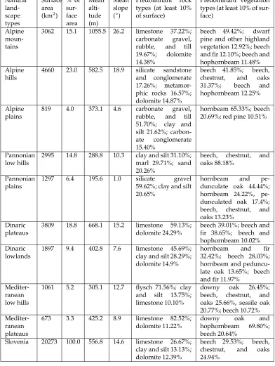
Natural land-scape types Surface area (km2)
% of sur-face area Mean alti-tude (m) Mean slope (◦) Predominant rock types (at least 10% of surface)
Predominant vegetation types (at least 10% of sur-face)
Alpine moun-tains
3062 15.1 1055.5 26.2 limestone 37.22%; carbonate gravel, rubble, and till 19.67%; dolomite 14.38%
beech 49.42%; dwarf pine and other highland vegetation 12.92%; beech and fir 12.10%; beech and hophornbeam 11.48% Alpine
hills
4660 23.0 582.5 18.9 silicate sandstone and conglomerate 17.26%; metamor-phic rocks 16.57%; dolomite 14.87%
beech 41.85%; beech, chestnut, and oaks 31.37%; beech and hophornbeam 12.25%
Alpine plains
819 4.0 373.1 4.6 carbonate gravel,
rubble, and till 51.70%; clay and silt 21.62%; carbon-ate conglomerate 15.40%
hornbeam 65.33%; beech 20.69%; red pine 10.51%
Pannonian low hills
2995 14.8 288.8 10.3 clay and silt 31.10%; marl 29.71%; sand 20.26%
beech, chestnut, and oaks 88.18%
Pannonian plains
1297 6.4 195.6 1.0 silicate gravel
59.62%; clay and silt 20.65%
hornbeam and
pe-dunculate oak 44.44%; hornbeam 24.22%, pe-dunculated oak 17.4%; beech, chestnut, and oaks 13.23%
Dinaric plateaus
3809 18.8 668.1 15.2 limestone 59.13%; dolomite 24.29%
beech 39.01%; beech and fir 38.65%; beech and hophornbeam 10.02% Dinaric
lowlands
1897 9.4 402.8 7.6 limestone 45.69%; clay and silt 28.29%; dolomite 14.9%
hornbeam and fir
32.42%; beech 28.03%; hornbeam and peduncu-late oak 13.65%; beech and fir 11.97%
Mediter-ranean low hills
1061 5.2 305.1 12.7 flysch 71.56%; clay and silt 13.75%; limestone 10.10%
downy oak 26.45%; beech, chestnut, and oaks 25.66%, sessile oak 20.77%; beech 10.72%
Mediter-ranean plateaus
673 3.3 425.2 8.9 limestone 82.52%;
dolomite 11.22%
downy oak and
hophornbeam 69.80%; beech 20.64%
Slovenia 20273 100.0 556.8 14.6 limestone 26.67%; clay and silt 13.13%; dolomite 12.39%
beech 29.53%; beech, chestnut, and oaks 24.94%
There were only four attempts to provide a suitable natural landscape classification of the country [32, 36, 38, 45]. In this paper, we focus on the well-established natural land-scape classification of Slovenia from 1998 [36], which is still used in the agriculture taxation process. Although the classification was the first partly computer-based natural landscape typology of Slovenia, the borders of landscape types were drawn manually.
Perko defined the core areas of each type by overlapping the digital layers of 7 surface elevation classes, 7 slope classes, 7 rock types, and 7 vegetation types. The slope and eleva-tion data were based on a 100-meter digital elevaeleva-tion model, and the lithology and vegeta-tion data were obtained through digitizavegeta-tion of 1:250,000 lithological and vegetavegeta-tion maps and converted to a 100-meter raster grid in order to prepare all the data layer in a raster format. Altogether, 2,401 different combinations were theoretically possible. He filtered the final layer three times using the modus inside of a moving 11 x 11 cell square win-dow, obtaining forty-eight larger and spatially separate homogenous cores with the same combination of elevation, slope, rock, and vegetation. He printed the forty-eight cores on a 1:250,000 scale map and manually drew borders between them, mostly following mor-phological boundaries and major watercourses. In the end, he combined these forty-eight manually delineated landscape units into nine natural landscape types (these are located in different areas and do not represent unique regions!), which he combined further into four natural landscape type groups (Table 1, Figure 1).
3
Data and methods
We propose a machine learning-based approach for understanding and quantitatively eval-uating the existing manually constructed classifications. We evaluated the consistency of Perko’s natural landscape classification (in this paper we will use term “original classifica-tion”) [36] by:
• modeling the original (existing) classification,
• producing a map of entropy (showing areas with high or low classification uncer-tainty), and
• determining which variables are the most influential (i.e., which natural elements explain the existing classification the best). We achieved the latter by applying a re-cently developed general black-box explanation method for explaining models’ pre-dictions [47]. The method is based on sensitivity analysis—perturbing the inputs and observing variability in the output—and can be applied to any prediction model.
Step 1. We use an automated train-test process to select the best-performing classifi-cation method from a set of machine learning and statistical algorithms for the training classification models, that is, the method that produces the models that best generalize the connection between the input variables (data layers) and landscape classification. The best rated method is then used to train a model using only the relevant input variables; that is, variable subset selection is also used (details are described in section 3.2).
Step 2. The model and the uncertainty of its predictions are used to interpret the original classification, primarily by analyzing the disagreements between the model and the origi-nal classification but also by the visualization of the entropy. Fiorigi-nally, a general method [47] for explaining how the input variables affect the classification is used on the model to pro-vide more insight into the concepts behind the model and the man-made classification (details are described in Section 3.3).
3.1
Data layers
In order to provide an explanatory model of the Slovenian natural landscape types, we had to take into consideration a set of 42 natural variables (data layers), which are inten-tionally different from the original Perko’s variables, and provide information on various environmental characteristics, such as relief, temperature, precipitation regime, and solar radiation. Original raster data layers were resampled to a cell resolution of 200 m, which was the lowest resolution of all the data layers. That provides 506,450 cells for the entire area. Vector layers were rasterized to the same resolution. All layers were trimmed to match the borders of the research area. The following input variables were included in the analysis:
• Elevation (m),
• Slope (◦),
• Aspect (north to south; 0–180◦),
• Elevation roughness coefficient (%),
• Slope roughness coefficient (%),
• Aspect roughness coefficient (%),
• Total roughness coefficient (%),
• Texture (share of cells in %),
• Annual temperature difference (◦C),
• Average annual temperature (◦C),
• Average monthly temperature (January–December,◦C),
• Difference between April and October temperatures (◦C),
• Average annual precipitation (mm),
• Average monthly precipitation (January–December, mm),
• Precipitation index (ratio between summer and fall precipitation),
• Precipitation index (ratio between summer and winter precipitation),
• Mediterranean precipitation index (difference between quantity of precipitation in October and November and quantity of precipitation in May and June multiplied by 100 and divided by annual quantity of precipitation [25]),
• Solar radiation (MJ/m2),
• River network density in 0.5 km radius (km/km2), and
• Bedrock permeability.
Relief data were derived from a digital relief model (provided by The Surveying and Mapping Authority of the Republic of Slovenia), climate data were calculated from data from the Slovenian Environment Agency, solar radiation was prepared by Gabrovec [19], and river network density was calculated from watercourse lines (provided by European Environment Information and Observation Network).
3.2
Model selection and data layer selection (Step 1)
The first phase of our process is an automatic construction of a model that connects the input variables with the original classification (target variable) using a set of algorithms. In machine learning, this problem is a standard prediction task with a categorical target variable (often referred to as a classification task). In our case, the target variable is a nat-ural landscape type. Numerous different methods for training models exist. However, no method is best for all problems, and it is impossible to determine beforehand which method will train the best model in our geographical setting and whether this might be different for different areas. Therefore, our aim in step 1 is to select the best method automatically from a set of commonly used classification methods.
It is not to be expected that even the best model will perfectly classify every point in every area. Disagreements (misclassifications) will occur for several reasons: the model be-ing unable to model the concepts used in the original classification, areas bebe-ing objectively difficult to classify into a single type, errors in the original classification, and errors in input variables. Therefore, the goal is to choose the model that has the least misclassifications or the best predictions.
Some methods are able to train very complex models, even up to the point of literally memorizing the classification of every point. This will lead to perfect or near-perfect pre-dictions on the data that were used for training the model, but because the model does not learn the actual concepts, poor predictions on new or unseen data from the same problem may occur. This is known as overfitting, and it is something that we want to avoid. Spa-tial data are especially problematic because the points are not independent—neighboring points reveal a lot about a point, even if that point is not included in the data that are used for learning.
In light of these facts, the model selection process (Figure 2, part 1A) was as follows. To avoid selecting a model that overfits the data, we used out-of-sample evaluation. To avoid overfitting due to spatial correlation, the data were sub-sampled—only a small percentage of the data points were included to increase the average distance between points. However, results were also reported for other degrees of sub-sampling.
Due to large amounts of data and difficulties of using cross-validation on spatial data due to spatial autocorrelation, we opted to use a train-test split evaluation. We ran the evaluation separately for each of the following numbers of training points: 2,500, 5,000, 10,000, 20,000, 50,000, and 100,000. For each run, the following was repeated 10 times: we selected the training points at random, and, also at random, 50,000 test points (no point was at the same time a test and a training point). For each repetition, the training points were used to train the model and the test points to estimate the classification error of the model. The errors were averaged across 10 repetitions to reduce noise in the error estimates. The criterion used for model selection was the log-score, a proper and local scoring rule, but classification accuracy is also reported. The log-score is defined as the logarithm of the probability that the model assigned to the true class and measures the quality of the predicted probabilities.
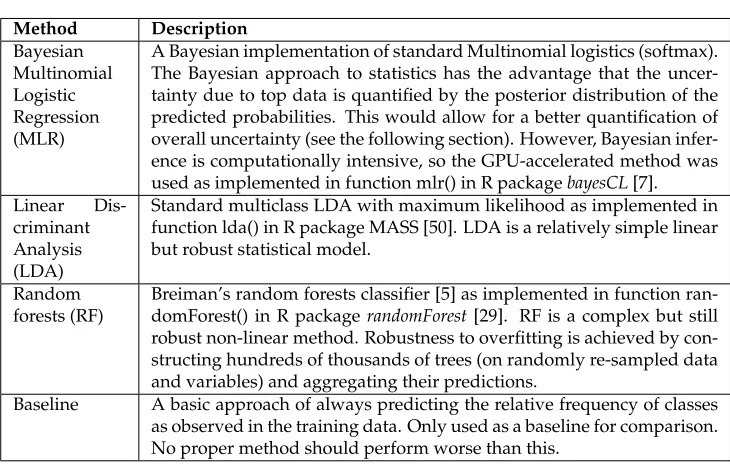
Method Description Bayesian Multinomial Logistic Regression (MLR)
A Bayesian implementation of standard Multinomial logistics (softmax). The Bayesian approach to statistics has the advantage that the uncer-tainty due to top data is quantified by the posterior distribution of the predicted probabilities. This would allow for a better quantification of overall uncertainty (see the following section). However, Bayesian infer-ence is computationally intensive, so the GPU-accelerated method was used as implemented in function mlr() in R packagebayesCL[7]. Linear
Dis-criminant Analysis (LDA)
Standard multiclass LDA with maximum likelihood as implemented in function lda() in R package MASS [50]. LDA is a relatively simple linear but robust statistical model.
Random forests (RF)
Breiman’s random forests classifier [5] as implemented in function ran-domForest() in R packagerandomForest[29]. RF is a complex but still robust non-linear method. Robustness to overfitting is achieved by con-structing hundreds of thousands of trees (on randomly re-sampled data and variables) and aggregating their predictions.
Baseline A basic approach of always predicting the relative frequency of classes as observed in the training data. Only used as a baseline for comparison. No proper method should perform worse than this.
Table 2: A description of the methods for learning classification models that were included in our experiments.
After the most appropriate method is selected and before explaining the model trained by that method, we also perform variable subset selection (Figure 2, part 1B). That is, in-put variables that do not contribute to the model’s predictive quality are removed from the model as part of pre-processing before generating the explanation. The main reason for variable selection is to simplify the explanation—while modern machine learning and statistical models are able to handle a large number of variables, people are still limited by the amount of information they can process.
We use a standard wrapper-based forward selection approach. That is, starting with 0 variables, the variables are added one at a time, at each step adding the variable that most improves the model’s predictive quality, to the point where the model’s predictive quality is indistinguishable from its predictive quality in the evaluation. As in the eval-uation process, the number of test samples was again 50,000 and the number of training samples 5,000, both sets were selected at random, the results were averaged across 10, and the log-score was used to measure prediction quality.
3.3
Model analyses (Step 2)
A single probabilistic prediction in classification is equivalent to assigning a distribution to a categorical random variable. As such, it is straightforward to use information-theoretic entropy as a measure of uncertainty of the model’s prediction for some pointj(Equation 1):
Hj=− n
X
i=1
pjilogpji (1)
wherepjiis the model’s predicted probability for classiandnis the number of classes. In this form, entropy is measured in bits. A 100% certain prediction (that is, a prediction where one of the predicted probabilitiespji is1and the rest are0) has0entropy, and the maximum entropy can be achieved by predicting uniformly across all classes (that is,pji= 1/nfor alli). A visualization ofHjfor all pointsjis referred to as an entropy map.
Another goal becomes to better understand how this model connects the variables and the original classification. To provide a sensible explanation of the model and its predic-tions, we post-processed the model using a general black-box explanation method (Figure 2, part 2C) that provides further insight into how the model works. In particular, we use a general black-box explanation method developed by Štrumbelj and Kononenko [47]. It can be applied to any type of prediction model. This method has some other advantages; in particular, it takes into account all possible interactions between input variables as opposed to explaining one variable at a time, as many general black-box explanations do.
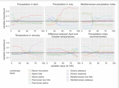
The method is based on a sensitivity analysis (changing the inputs and observing changes in the output) and can therefore be applied to a trained model, without any need to re-train the model. The explanations are based on variable contributions (how much vari-ables’ values contribute to or against a certain prediction). The explanation of the model (see Figure 5) provides an overview of how values of the input variables influence the model’s predictions. It includes, for each variable, a plot of how the importance of that variable varies across its values. Each line represents a class value (in our case landscape type). A positive importance value indicates that the value supports that class value, and a negative value does not support that class value.
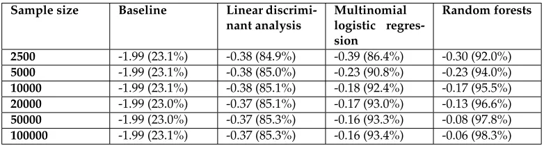
Sample size Baseline Linear
discrimi-nant analysis
Multinomial logistic regres-sion
Random forests
2500 -1.99 (23.1%) -0.38 (84.9%) -0.39 (86.4%) -0.30 (92.0%)
5000 -1.99 (23.1%) -0.38 (85.0%) -0.23 (90.8%) -0.23 (94.0%)
10000 -1.99 (23.1%) -0.38 (85.1%) -0.18 (92.4%) -0.17 (95.5%)
20000 -1.99 (23.0%) -0.37 (85.1%) -0.17 (93.0%) -0.13 (96.6%)
50000 -1.99 (23.0%) -0.37 (85.3%) -0.16 (93.3%) -0.08 (97.8%)
100000 -1.99 (23.1%) -0.37 (85.3%) -0.16 (93.4%) -0.06 (98.3%)
4
Results
4.1
Model selection
Model selection results are shown in Table 3. The random forests method was selected be-cause it outperformed all the other methods for all training sample sizes. All further results were obtained using random forests and the training sample size of 5000 (representing 1% of the total area). The smaller number of training samples was used to prevent overfitting due to the spatial autocorrelation.
4.2
Final variable selection
During variable subset selection, six of 42 variables (data layers) were found to be relevant to the predictions of the random forests method:
• precipitation in April,
• precipitation in July,
• precipitation index (ratio between summer and fall precipitation),
• temperature in January,
• Mediterranean precipitation index (difference between quantity of precipitation in October and November and quantity of precipitation in May and June multiplied by 100 and divided by annual quantity of precipitation [25], and
• difference between April and October temperatures (Figure 3).
4.3
Model analyses—discrepancies and uncertainties
Figure 4: A map of entropy (in bits). Darker areas represent areas where there is more uncertainty in the model’s classifications.
4.4
Model analyses—explanation of how the input variables affect the
model’s predictions
The general black-box explanation method for explaining variable importance provided variable importance plots (Figure 5). The plots explained the variable importance of each variable according to its values for the determination of each specific natural landscape type. The output makes it possible to interpret the existing landscape classifications in greater detail.
5
Discussion
5.1
Possibilities of spatial evaluation of the natural landscape
classifica-tion
Figure 5: The general method for explaining variable importance provides insight into the connection between the input variables and the predicted probability of a particular natural landscape type. The graphs provide an overview of how values of the input variables in-fluence the model’s predictions. The explanation includes, for each variable, a plot of how the importance of that variable differs across its values. Each line represents a class value (in our case natural landscape type). A positive importance value indicates that the value supports that class value, and a negative value indicates that it does not support that class value. For instance, let us demonstrate how variable temperature in January (bottom left graph) helps to classify the Alpine mountains (red line). We can see that low temperature values in January (x-axis: values that are lower than 50) have positive variable importance for the determination of the Alpine mountains. This means that low temperatures speaks in favor of the Alpine mountains.
other methods (statistical models and decision trees) were less successful—with up to 75% agreement [9]. This can be explained by a larger number of variables used and a more complex model (random forests).
differ from those low-hill and plain areas in vicinity due to their higher altitude and their climate characteristics (higher rate of precipitation, lower temperature). Due to quite dis-tinct differences, high uncertainty has its origin in actual mistakes made during the man-ual creation of the original classification. On the other hand, the Dinaric plateaus are very similar to the Dinaric lowlands. The latter have similar precipitation regimes and similar amount of precipitation. Therefore, these uncertainties are more a result of a true similarity of the two natural landscape types.
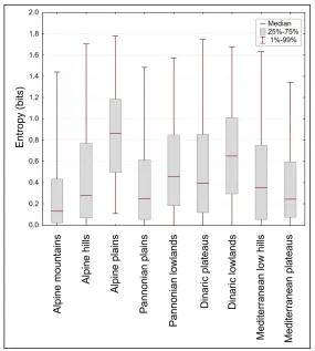
We also visually checked box-plots of entropy for each natural landscape type (Figure 6) in order to find the most complex type. Surprisingly, Alpine plains have the highest entropy on average. One of the main reasons is that these landscape types are located in two separate areas, which have a different value of the precipitation index. High entropy is also a consequence of some hilly areas inside the type. Similarly, Pannonian plains also have high entropy (3rd highest average entropy). Dinaric lowlands are the 2nd hardest to classify. This is due to the facts that the type is quite diverse and that includes Ljubljana moor, karst poljes, karst plains, and some lower parts of karst hills. Additionally, the land-scape type is also diverse from the climatic point of view. It spreads from the west towards the east, and it represents a transitional area between the Mediterranean and Continental climate, making classification even more difficult (see also Figure 1).
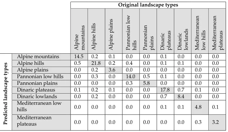
Most of the mistakes are related to similar landscape types (Table 4). For example, Dinaric plateaus and Dinaric lowlands have very rough terrain with numerous dolines and an absence of a surface fluvial system. Therefore, it is harder to differentiate between larger landforms there than in fluvial landscapes with distinct valleys and ridges.
Original landscape types
Alpine mountains Alpine
hills
Alpine
plains
Pannonian
low
hills Pannonian plains Dinaric plateaus Dinaric lowlands Mediterranean low
hills
Mediterranean plateaus
Alpine mountains 14.5 0.2 0.1 0.0 0.0 0.1 0.0 0.0 0.0
Alpine hills 0.5 21.8 0.2 0.4 0.0 0.1 0.1 0.0 0.0
Alpine plains 0.0 0.2 3.6 0.0 0.0 0.0 0.0 0.0 0.0
Pannonian low hills 0.0 0.3 0.0 14.0 0.5 0.1 0.0 0.0 0.0
Pannonian plains 0.0 0.0 0.0 0.3 5.8 0.0 0.0 0.0 0.0
Dinaric plateaus 0.1 0.2 0.1 0.0 0.0 17.8 0.7 0.1 0.0
Dinaric lowlands 0.0 0.2 0.0 0.0 0.0 0.7 8.4 0.0 0.0
Mediterranean low
hills 0.0 0.0 0.0 0.0 0.0 0.1 0.1 4.8 0.1
Predicted
landscape
types
Mediterranean
plateaus 0.0 0.0 0.0 0.0 0.0 0.0 0.0 0.3 3.2
Table 4: Confusion matrix (%) for landscape type classification shows the most frequent pairs of misclassification.
One of the most important parts of our research is the explanation of the variable se-lection (Figure 5). At the time of constructing the original natural landscape classification, the following elements that influenced the formation of types were elevation, slope, rocks, and vegetation. Our analysis did not take into account any other knowledge or perception about the country and focused purely on digital values of the data layers. At first, the list of selected explanatory variables (see Section 4.2) for modeling was surprising. Namely, a lot of geographical research regarding natural landscape classification is tightly connected to landforms (geomorphology), including elevation and slope.
Random forests modeling and further explanation of variable importance, in our case, partially disproved the importance of most of geomorphological data layers at this level of natural landscape classification, at least directly. Six data layers (precipitation in April, pre-cipitation in July, prepre-cipitation index, temperature in January, Mediterranean prepre-cipitation index and the difference between April and October temperatures) were used to train the classification model. All layers are climate variables. The original climate layers were inter-polated from ground meteorological stations [15] and thus provided a gentler (not noisy) surface.
it was also used in the modeling of temperature and precipitation maps [15]. Therefore, the elevation layer is highly correlated with the difference between April and October temper-atures and also temperature in January.
These findings are also supported by other analysis [10]. According to their research on scale, climatic variables and elevation were classified in the same group of variables, which are more appropriate for classification at the national scale (Slovenia covers approximately 20,000 km2). On the other hand, geomorphological properties (e.g., slope) were defined as more appropriate on a larger scale covering smaller, local area.
Therefore, we confirm that climate variables can sufficiently represent the original nat-ural landscape classification and that surface configuration is less important, with an ex-ception of elevation, which has an indirect influence.
Graphical and statistical revision of the data layers included in the model (Figure 3) and their importance (Figure 5) revealed that we can define distinct rules for the definition of groups of natural landscape types and most individual natural landscape types. The Alpine mountains are determined by high April and July precipitation values and also low January temperature values. The Pannonian landscapes stand out due to the low April precipitation values and high difference between April and October temperatures. The Mediterranean landscapes have low July precipitation values and high January tempera-tures. There are some situations that cannot be easily described. These are differentiations between the following:
• Mediterranean low hills and Mediterranean plateaus,
• Pannonian low hills and Pannonian plains, and
• Dinaric plateaus and Dinaric lowlands.
In general, modeling produced reasonable results that are highly similar to the origi-nal classification, and most of the explanations of the natural landscape types also have a logical geographical background.
5.2
An assessment of the method and its capabilities
The classification phase of the presented machine learning-based approach did not have any issues or limitations in this geographical setting. The models were able to achieve high classification accuracy and quality of probabilistic predictions. Random forests were the best, and it is reasonable to assume that will often be the case in this setting, even if other areas or classifications are evaluated. However, even if this is not the case, any other classifier can be used in this phase, due to the generality of the general black-box explanation method in the second phase of the process.
purely because humans are also limited in how many variables they can take into account. Therefore, the general black-box explanation method is suitable for this setting.
We were able to confirm most of the computer explanation and understand the main reasons for divisions between the natural landscape types; however, some pairs of natural landscape types were hard to easily differentiate (see Section 5.1). The data also possess a certain degree of noise (e.g., due to the interpolation of climate data). Also note that the general black-box explanation method, while taking into account all interactions between input variables when determining their importance, reports only one variable importance number per variable (layer). While the method itself can easily be generalized to report importance for each pairwise interaction (or higher level interactions), these can quickly become difficult or even impossible for the user to interpret. Random forests tend to have many higher level interactions, which could explain why for certain cases a reasonable geographical explanation was not possible. It is in the structure of decision-tree based models that every node depends on all the prior tree splits on the path from the root to the node, which results in interactions.
5.3
Broader implications of the results and relation to previous results
The main challenge was to explain the existing natural landscape classification of Slovenia, as other authors did for Norway and Hungary [33, 46]. For one part of Slovenia, a similar evaluation with machine learning modeling was done for “Karst landscape of the interior of Slovenia” [6] and for the entire country [9], but these analyses have not explained vari-able importance of the selected varivari-ables. Since the selection of varivari-ables is important [55], our paper brought a deeper understanding of Slovenian natural landscape types that also includes model explanation.
“completely objective” classes. A similar study was done for the climate classification of Slovenia [26]. The results of an unsupervised classification were similar to some of the older climatic classifications. Therefore, a similar approach has also been tested for the nat-ural landscape classification [37]. The comparison between modeled classifications and the original have shown that models, according to the unsupervised classification methods, achieved lower rates of agreement, which was expected. However, this also means that unsupervised classifications revealed the fact that the original classification could also be designed in a different way.
5.4
Practical application
In our research, modeling confirmed that existing natural landscape classification is made with great sense. The classification can mostly be described with logical statements, al-though the original classification was determined on the basis of other data mainly with manual delimitation. In the case that the original classification was irrational, the models would not be able to form [8]! Our results also provided information on areas with high entropy. Those areas can be further investigated (also in the field) in order to correct the original classification.
Since the classification we analyzed is also used for official purposes of agricultural land taxation [57], our results can be useful for improving classification (e.g., for correction of the borders between plain and hilly landscape types) by repeating the process at a higher reso-lution (e.g., 25 m, in case all the data layers are available at such resoreso-lution). Another option is to produce a detailed landform classification first and then use it as a starting point for subsequent classification of complex land surface features [14], especially if adding data on other landscape elements. However, using such methods for providing corrections would contribute to a better and more effective distribution of taxes and subsidies and thus to a fairer society.
6
Conclusion
Natural landscape classifications are important for a suitable understanding of the envi-ronment. Therefore, they must be prepared with great care, especially if they have a di-rect impact on official regulations and policy. Therefore, the main aim of the paper was to introduce and test new approaches for natural landscape classification evaluation us-ing machine learnus-ing. By modelus-ing existus-ing classifications with random forests and with the general black-box explanation method for explaining variable importance, we were able to analyze how the existing manually defined natural landscape classification can be (re)produced and explained with machine learning algorithms. The new approach was tested for the case of Perko’s [36] natural landscape classification of Slovenia, which is used in the official taxation process.
The analysis with the general black-box explanation method provided insight into how different variables influence the classification of natural landscape types. Most of the au-tomated explanation was logical and was confirmed by the analysis of the geographical characteristics of the research area. Therefore, a selection of variables proved to be rea-sonable, although a set of exclusively climatic variables was not expected. Namely, many landscape researchers usually give most attention to geomorphological variables. The se-lection of variables for modeling at the national level was eventually proved to be correct; climate variables are more general than geomorphological variables, and some of them are also correlated with elevation; thus, elevation was not included as an independent vari-able. However, the detailed evaluation of variables revealed differences between natural landscape types, which were reasonable and in most cases easy to explain. The method did not provide clear explanations for some differentiations between landscape types with very similar characteristics.
The process of modeling and evaluating that we propose addresses important natural landscape classification issues, especially transparency and evaluation. The process can evaluate different numeric models and is reproducible. The results can show the classifica-tion probability and what affects it. They can also explain the influence of specific charac-teristics (variables) of a natural landscape classification. Finally, the discrepancies between an original and a model and also areas with high entropy can also help us to improve clas-sification and to diminish subjectivity. Therefore, the methodology could become a useful tool for natural landscape classification evaluation. Lastly, the use of the approach is an example of how modern methods in landscape ecology, geography and related sciences can improve landscape management and increase financial fairness.
Acknowledgments
The authors acknowledge financial support from the Slovenian Research Agency (project no. L1-7542: Advancement of computationally intensive methods for efficient modern general-purpose statistical analysis and inference; program no. P6-0101: Geography of Slovenia).
References
[1] BAILEY, R. G. Ecosystem geography. Springer, New York, 1996.
[2] BAILEY, R. G. Identifying Ecoregion Boundaries. Environmental Management 34, S1 (2004), S14–S26. doi:10.1007/s00267-003-0163-6.
[3] BERGINC, M., KREMESECJEVŠENAK, J.,ANDVIDIC, J.Sistem varstva narave v Sloveniji. Ministrstvo za okolje in prostor, Ljubljana, 2007.
[4] BOHN, U., NEUHÄUSL, R., GOLLUB, G., HETTWER, C., NEUHÄUSLOVÁ, Z., RAUS, T., SCHLÜTER, H.,ANDWEBER, H., Eds.Karte der Natürlichen Vegetation Europas/Map of the Narural Vegetation of Europe, 1. aufl ed. Bundesamt für Naturschutz, Münster, 2003.
[6] BRESKVARŽAUCER, L.,ANDMARUŠI ˇC, J. Analiza krajinskih tipov z uporabo umet-nih nevronskih mrež.Geodetski vestnik 50, 2 (2006), 224–237.
[7] ˇCEŠNOVAR, R.,ANDŠTRUMBELJ, E. Bayesian Lasso and multinomial logistic
regres-sion on GPU.PLOS ONE 12, 6 (2017), e0180343. doi:10.1371/journal.pone.0180343.
[8] CIGLI ˇC, R. Assessing the impact of input data incongruity in selected quantitative methods for modelling natural landscape typologies. Geografski vestnik 90, 1 (2018), 115–141. doi:10.3986/GV90107.
[9] CIGLI ˇC, R., AND PERKO, D. Modelling as a Method for Evaluating Natural Land-scape Typology: The Case of Slovenia. InLandscape Analysis and Planning, M. Luc, U. Somorowska, and J. Szma ´nda, Eds. Springer International Publishing, Cham, 2015, pp. 59–79. doi:10.1007/978-3-319-13527-4_4.
[10] CIGLI ˇC, R., AND PERKO, D. A method for evaluating raster data layers ac-cording to landscape classification scale. Ecological Informatics 39 (2017), 45–55. doi:10.1016/j.ecoinf.2017.03.004.
[11] CONGALTON, R. G. A review of assessing the accuracy of classifications of remotely sensed data. Remote Sensing of Environment 37, 1 (1991), 35–46. doi:10.1016/0034-4257(91)90048-B.
[12] CULLUM, C., ROGERS, K. H., BRIERLEY, G.,ANDWITKOWSKI, E. T. Ecological clas-sification and mapping for landscape management and science: Foundations for the description of patterns and processes. Progress in Physical Geography: Earth and Envi-ronment 40, 1 (2016), 38–65. doi:10.1177/0309133315611573.
[13] DE MERS, M. N. Teaching the complexities of map boundaries. In Teaching Spa-tial Thinking from Interdisciplinary Perspectives, 12 October, Santa Fe(Santa Fe, 2015), H. Burte, T. Kauppinen, and M. Hegarty, Eds., vol. 1557, CEUR-WS.org, pp. 21–24.
[14] DEKAVALLA, M., AND ARGIALAS, D. Evaluation of a spatially adaptive
approach for land surface classification from digital elevation models. In-ternational Journal of Geographical Information Science 31, 10 (2017), 1978–2000. doi:10.1080/13658816.2017.1344984.
[15] DOLINAR, M. Monthly gridded datasets for temperature and precipitation over
Slove-nia. InProceedings of GeoMLA—Geostatistics and Machine Learning, 21-24 June, Belgrade
(Belgrade, 2016), M. Kilibarda and J. Lukovi´c, Eds., Faculty of Civil Engineering, Uni-versity of Belgrade, p. 17.
[16] DR ˇAGU ¸T, L., AND EISANK, C. Automated object-based classification of topography from SRTM data. Geomorphology 141-142 (2012), 21–33. doi:10.1016/j.geomorph.2011.12.001.
[17] ERIKSTAD, L., UTTAKLEIV, L. A., AND HALVORSEN, R. Characterisation and mapping of landscape types, a case study from Norway. Belgeo, 3 (2015), 1–16. doi:10.4000/belgeo.17412.
[18] FNUKALOVÁˇ , E., AND ROMPORTL, D. A typology of natural landscapes of Central
[19] GABROVEC, M. Solar Radiation and the Diverse Relief of Slovenia/Sonˇcno obsevanje v reliefno razgibani Sloveniji.Geografski zbornik/Acta geographica 36(1996), 47–68.
[20] HAGGETT, P. Geography: a global synthesis. Prentice Hall an imprint of Pearson Educa-tion, Harlow, 2001.
[21] HALL, A., AHONEN-RAINIO, P.,ANDVIRRANTAUS, K. Insight provenance for spa-tiotemporal visual analytics: Theory, review, and guidelines.Journal of Spatial Informa-tion Science, 15 (2017), 65–88. doi:10.5311/JOSIS.2017.15.337.
[22] JAN, S., SCHWERING, A., SCHULTZ, C.,ANDCHIPOFYA, M. C. Cognitively plausible representations for the alignment of sketch and geo-referenced maps.Journal of Spatial Information Science, 14 (2017), 31–59. doi:10.5311/JOSIS.2017.14.294.
[23] JONGMAN, R. H. G., BUNCE, R. G. H., METZGER, M. J., MÜCHER, C. A., HOWARD, D. C.,ANDMATEUS, V. L. Objectives and Applications of a Statistical Environmental Stratification of Europe. Landscape Ecology 21, 3 (2006), 409–419. doi:10.1007/s10980-005-6428-0.
[24] KONONENKO, I., ŠTRUMBELJ, E., BOSNI ´C, Z., PEVEC, D., KUKAR, M.,ANDROBNIK
-ŠIKONJA, M. Explanation and reliability of individual predictions. Informatica 37, 1 (2013), 41–48.
[25] KOPPÁANY, G., AND UNGER, J. Mediterranean Climatic Character in the Annual March of Precipitation. Acta Climatologica 34-36(1992), 59–71.
[26] KOZJEK, K., DOLINAR, M.,ANDSKOK, G. Objective climate classification of Slovenia.
International Journal of Climatology 37, S1 (2017), 848–860. doi:10.1002/joc.5042.
[27] KUNÁKOVÁ, L., ŠTEFKO, R.,AND BA ˇCÍK, R. Evaluation of the landscape potential for recreation and tourism on the example of microregion Minˇcol (Slovakia).e-Review of Tourism Research 2, 1/2 (2016), 335–354.
[28] LAUSCH, A., BLASCHKE, T., HAASE, D., HERZOG, F., SYRBE, R.-U., TISCHENDORF, L.,ANDWALZ, U. Understanding and quantifying landscape structure—A review on relevant process characteristics, data models and landscape metrics. Ecological Mod-elling 295(2015), 31–41. doi:10.1016/j.ecolmodel.2014.08.018.
[29] LIAW, A.,ANDWIENER, M. Classification and Regression by randomForest. R News 2/3(2002), 18–22.
[30] LOVELAND, T. R., AND MERCHANT, J. M. Ecoregions and Ecoregionalization: Ge-ographical and Ecological Perspectives. Environmental Management 34, S1 (2004), S1– S13. doi:10.1007/s00267-003-5181-x.
[31] LU, D., AND WENG, Q. A survey of image classification methods and techniques for improving classification performance. International Journal of Remote Sensing 28, 5 (2007), 823–870. doi:10.1080/01431160600746456.
[33] MEZ ˝OSI, G. Similarity assessment of natural landscapes based on taxonomic distance. Applied Ecology and Environmental Research 14, 3 (2016), 679–693. doi:10.15666/aeer/1403_679693.
[34] MÜCHER, C. A., BUNCE, R. G. H., JONGMAN, R. H. G., KLIJN, J. A., KOOMEN, A. J. M., METZGER, M. J.,ANDWASCHER, D. M. Identification and Characterisation of
Environments and Landscapes in Europe. Tech. rep., Alterra, Wageningen, 2003.
[35] PEDROLI, B., PINTO-CORREIA, T., AND CORNISH, P. Landscape—What’s in it? Trends in European Landscape Science and Priority Themes for Concerted Research.
Landscape Ecology 21, 3 (2006), 421–430. doi:10.1007/s10980-005-5204-5.
[36] PERKO, D. The Regionalization of Slovenia. Geografski zbornik/Acta geographica 38
(1998), 11–57.
[37] PERKO, D., CIGLI ˇC, R., AND HRVATIN, M. The usefulness of unsupervised
classi-fication methods for landscape typiclassi-fication: The case of Slovenia. Acta geographica Slovenica 59, 2 (2019), 7–26. doi:10.3986/AGS.7377.
[38] PERKO, D., HRVATIN, M., AND CIGLI ˇC, R. A methodology for natural land-scape typification of Slovenia. Acta geographica Slovenica 55, 2 (2015), 235–270. doi:10.3986/AGS.1938.
[39] PLUT, D. Regionalizacija Slovenije po sonaravnih kriterijih. Geografski vestnik 71
(1999), 9–25.
[40] REES, P. W., AND LEGATES, M. Returning “region” to world regional ge-ography. Journal of Geography in Higher Education 37, 3 (2013), 327–349. doi:10.1080/03098265.2013.769089.
[41] RIBEIRO, D., SOMODI, I., AND CˇARNI, A. Transferability of a predictive Robinia pseudacacia distribution model in northeast Slovenia.Acta geographica Slovenica 56, 1 (2016), 25–43. doi:10.3986/AGS.772.
[42] RIU-BOSOMS, C., VIDAL, T., DUANE, A., FERNANDEZ-LLAMAZARESONRUBIA, A., GUEZE, M., LUZ, A. C., PANEQUE-GÁLVEZ, J., MACIA, M. J.,ANDREYES-GARCIA, V. Exploring Indigenous Landscape Classification across Different Dimensions: A Case Study from the Bolivian Amazon. Landscape Research 40, 3 (2015), 318–337. doi:10.1080/01426397.2013.829810.
[43] ROBA, H. G., ANDOBA, G. Community participatory landscape classification and biodiversity assessment and monitoring of grazing lands in northern Kenya. Journal of Environmental Management 90, 2 (2009), 673–682. doi:10.1016/j.jenvman.2007.12.017.
[44] ROCCHINI, D.,ANDRICOTTA, C. Are landscapes as crisp as we may think?Ecological Modelling 204, 3-4 (2007), 535–539. doi:10.1016/j.ecolmodel.2006.12.028.
[45] ŠPES, M., CIGALE, D., LAMPI ˇC, B., NATEK, K., PLUT, D.,ANDSMREKAR, A. Študija ranljivosti okolja.Geographica Slovenica 35, 1–2 (2002), 1–150.
[47] ŠTRUMBELJ, E.,ANDKONONENKO, I. Explaining prediction models and individual predictions with feature contributions. Knowledge and Information Systems 41, 3 (2014), 647–665. doi:10.1007/s10115-013-0679-x.
[48] UDVARDY, M. D. F. A classification of the biogeographical provinces of the World. Tech. rep., International union for conservation of nature and natural resources, Morges, 1975.
[49] URBANC, M., GAŠPERI ˇC, P., AND KOZINA, J. Geographical imagination of land-scapes: analysis of the book of photographs Slovenian landscapes. Acta geographica Slovenica 55, 1 (2015), 99–125. doi:10.3986/AGS.836.
[50] VENABLES, W. N., AND RIPLEY, B. D. Modern applied statistics with S, 4th ed ed. Statistics and computing. Springer, New York, 2002.
[51] VENABLES, W. N.,ANDRIPLEY, B. D. An Introduction to R. 2018.
[52] WARNOCK, S., AND GRIFFITHS, G. Landscape Characterisation: The Living Landscapes Approach in the UK. Landscape Research 40, 3 (2015), 261–278. doi:10.1080/01426397.2013.870541.
[53] WASCHER, D. M. Landscape character: linking space and function. InEuropean Land-scape Character Areas. Typologies, cartography and indicators for the assessment of sustainable landscapes, D. M. Wascher, Ed. Landscape Europe, Wageningen, 2005, pp. 1–4.
[54] WIECZOREK, M., AND MIGO ´N, P. Automatic relief classification versus ex-pert and field based landform classification for the medium-altitude moun-tain range, the Sudetes, SW Poland. Geomorphology 206 (2014), 133–146. doi:10.1016/j.geomorph.2013.10.005.
[55] WILLIAMS, K. J., BELBIN, L., AUSTIN, M. P., STEIN, J. L., AND FERRIER, S.
Which environmental variables should I use in my biodiversity model? In-ternational Journal of Geographical Information Science 26, 11 (2012), 2009–2047. doi:10.1080/13658816.2012.698015.
[56] WILLIAMS, M., KUHN, W., AND PAINHO, M. The influence of landscape varia-tion on landform categorizavaria-tion. Journal of Spatial Information Science, 5 (2012), 51–73. doi:10.5311/JOSIS.2012.5.107.