RESEARCHARTICLE
A cutting-plane method for
contiguity-constrained spatial
aggregation
Johannes Oehrlein and Jan-Henrik Haunert
Institute of Geodesy and Geoinformation, University of Bonn, Germany
Received: September 11, 2016; returned: November 17, 2017; revised: November 26, 2017; accepted: November 28, 2017.
Abstract: Aggregating areas into larger regions is a common problem in spatial planning, geographic information science, and cartography. The aim can be to group administrative areal units into electoral districts or sales territories, in which case the problem is known as districting. In other cases, area aggregation is seen as a generalization or visualization task, which aims to reveal spatial patterns in geographic data. Despite these different motiva-tions, the heart of the problem is the same: given a planar partition, one wants to aggregate several elements of this partition to regions. These often must have or exceed a particular size, be homogeneous with respect to some attribute, contiguous, and geometrically com-pact. Even simple problem variants are known to be NP-hard, meaning that there is no reasonable hope for an efficient exact algorithm. Nevertheless, the problem has been at-tacked with heuristic and exact methods. In this article we present a new exact method for area aggregation and compare it with a state-of-the-art method for the same problem. Our method results in a substantial decrease of the running time and, in particular, allowed us to solve certain instances that the existing method could not solve within five days. Both our new method and the existing method use integer linear programming, which allows existing problem solvers to be applied. Other than the existing method, however, our method employs a cutting-plane method, which is an advanced constraint-handling approach. We discuss this approach in detail and present its application to the aggregation of areas in choropleth maps.
1
Introduction
Planar subdivisions are frequently used to structure geographic space. In geographic in-formation systems, they can be used as a basis for data acquisition, storage, analysis, and visualization. Since different applications require information on different scales, planar subdivisions are often hierarchical—unemployment rates, for example, can be analyzed on a county or country level. Often, one aims to compute a higher-level subdivision from a given one, by grouping areas of similar attribute values. With such an approach, one can reveal large-scale patterns in the data. In this article, we present a new method for area aggregation, which we discuss in the context of districting and spatial unit allocation. We distinguish these problems as follows:
• Districting[9, 36, 38, 62] is the problem of partitioning a set of minimum mapping units (e.g., postal code zones) to form larger regions or districts (e.g., school zones or electoral districts). The minimum mapping units (i.e., input areas) are assumed to form a planar subdivision. The applications of districting range from administrative to commercial purposes; an overview is provided by Shirabe [61].
• Spatial unit allocation[60, 61] subsumes districting, but it does not necessarily ask to assign every area to a district. A typical example of spatial unit allocation is to select a set of areas constituting a single region that is geometrically compact and requires minimal development costs [1].
• The termarea aggregationhas been used to refer to the aggregation of areas as a data abstraction or map generalization problem [34]. Just as districting, area aggregation requires a planar subdivision as input and asks to group the areas into larger regions. Districting problems in spatial planning, however, do not necessarily ask to group areas of similar attribute values, which is an essential criterion for generalization.
It is common to approach districting, spatial unit allocation, and area aggregation by optimization [7, 20, 29, 33, 45, 49, 62]. The existing approaches are quite similar, since the different problem variants often share some optimization objectives and constraints. For example, it is common to require that every output region must have a size or population within certain bounds and to favor geometrically compact shapes. Compactness is usually assessed quantitatively, which can be done with different measures [44,47], and considered as an optimization objective. Additionally, in many problem variants, the output regions are required to becontiguous[14, 20, 61, 62, 69]:
Definition 1. An areaA ⊆R2is calledcontiguousif every two points inAare connected via a (not necessarily straight) line that is contained inA.
Though the output regions tend to become contiguous when compactness is considered as an objective, there is generally no guarantee for contiguity without enforcing it. In fact, if compactness is not the primary objective, contiguity often has to be enforced to produce somehow reasonable output regions [62]. Therefore, we think that optimizing similarity (and compactness as a secondary criterion) subject to size constraints and contiguity is a particularly interesting challenge.
v1 v2 v3
v4 v5 v6
v7 v8 v9
(a) Explanatory maps: input map (left) and out-put map (right).
(b) The adjacency graphG= (V, E)for the input map in (a) and the partition ofV corresponding to the output map.
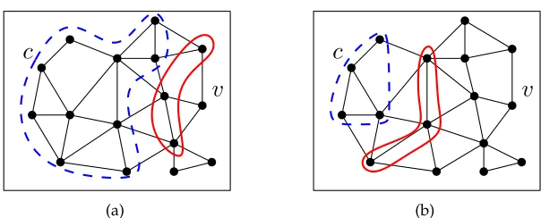
Figure 1: An example of area aggregation (see Haunert and Wolff [34]).
and output representations are visual graphics. Haunert and Wolff [34] have defined the area aggregation problem in map generalization formally and developed an optimization method for it, which is based on models for districting by Zoltners and Sinha [70] and Shirabe [62]. The problem not only requires to group the input areas into larger regions, but also to assign a value from the attribute domain to each output region; see Figure 1(a). The aim is to minimize a cost function that penalizes changes of attribute values to dis-similar values as well as geometrically non-compact output regions, subject to constraints concerning the size and contiguity of the output regions. The method relies on the defini-tion of the adjacency graphG= (V, E)whose vertex setV contains a vertex for each input area and whose edge setEcontains an edge{u, v}for each two adjacent areasu, v∈V; see Figure 1(b). We will use this definition ofGthroughout this article.
In this article, we revisit the problem defined by Haunert and Wolff [34], but we also consider the special case that similarity is neglected and compactness is the sole objec-tive. In this case, the problem is more similar to a classical districting problem that simply demands geometrically compact and contiguous regions of sizes within certain bounds. Moreover, while Haunert and Wolff developed and tested their method for the general-ization of categorical maps, we will use our method to generalize choropleth maps with a ratio-scaled variable, such as unemployment rates. This has the advantage that we can directly compute differences between attribute values and do not depend on the definition of a semantic distance between categories.
We focus onexactoptimization methods based oninteger linear programming, which is a common optimization approach for districting [9, 33, 36]. In particular, it is reasonable for NP-hard problems, for which the existence of an efficient and exact algorithm is extremely unlikely [28]. In fact, area aggregation falls into the class of NP-hard problems [34], and so do many problem variants of districting [2, 38, 57].
x2
x1
1 1
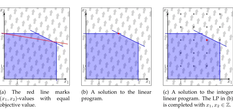
(a) The red line marks
(x1, x2)-values with equal objective value.
x2
x1
1 1
(b) A solution to the linear program.
x2
x1
1 1
(c) A solution to the integer linear program. The LP in (b) is completed withx1, x2∈Z. Figure 2: A linear program with variablesx1andx2; objective is to maximize6x1+x2with respect to
x1≥0,x2≥0,2x2≤7,2x1+4x2≤18andx1≤4. The solution space, i.e., all pairs(x1, x2)for which every given inequality is true, is marked as a blue polytope. The gray arrows in the background indicate the objective. They are orthogonal to the line of equal objective values in (a).
Whereas efficient algorithms for linear programming exist, integer linear ming is NP-hard [13, 28]. Nevertheless, an approach based on integer linear program-ming is promising as it allows sophisticated optimization software (e.g., CPLEX [15] and Gurobi [31]) to be applied. Even though the exact methods for solving ILPs have an ex-ponential worst-case running time, they can be relatively fast when applied to real-world instances. Moreover, solutions of an exact method can be used as quality benchmarks to evaluate the results of (faster) heuristic algorithms. Heuristic methods for districting have been developed by several researchers [7, 19, 37, 43, 50]. In contrast to exact methods, these do not guarantee to deliver an optimal solution.
Just as some criteria are shared by many problem variants of districting and spatial unit allocation, the ILP formulations for these problems often share some elementary compo-nents. Shirabe [63] has used this fact to integrate mathematical programming techniques and geographic information systems (GIS), such that a GIS user can assemble a model for a particular spatial unit allocation problem from a set of elementary model components and compute a solution to the problem with an ILP solver. Since contiguity is an impor-tant requirement in many spatial unit allocation problems, several works have focused on formalizing contiguity as one such elementary model component [61, 62, 69].
Usually, there exist multiple possibilities of encoding a particular problem as an ILP; choosing among these ILP formulations can highly influence the computation time. In ge-ographic information (GI) science, it is common to choose acompactILP formulation, which means that the size of the ILP is polynomial in the size of the input [24]. For example, in Section 2.2 we show that, when applying Shirabe’s model [61] to area aggregation without prescribing the number of output regions, it hasO(n2)variables and constraints (wherenis
be handed over to a solver, which computes an optimal solution without requiring any further interaction. It is therefore common to think of the solver as a black box [46].
Working with compact ILP formulations is relatively convenient. It is also known, how-ever, that they are sometimes outperformed bynon-compactILP formulations, whose num-ber of constraints can be exponential in the size of the input [56]. Such a large set of con-straints forbids a full instantiation of the model. Therefore, one starts the computation by working with a reduced ILP, which is lacking a set of constraints of the original ILP. A sim-ple approach is to solve this reduced ILP to optimality and to examine whether the solution violates constraints of the original ILP. If a violation of a constraint is found, that constraint is added to the ILP and the solution process is started anew. Drexl and Haase [18] and Duque et al. [20] use this approach to solve districting problems. In particular, Duque et al. deal with thep-regions problem, in which, other than in our problem, the number pof output regions is prescribed.
In this article, we present a more sophisticated approach for area aggregation. We demonstrate the effectiveness of acutting-plane method, which generally refers to a method that adds constraints during optimization without relying on an optimal solution to the reduced ILP. Violated constraints are found already in a preliminary stage of a solution, namely in an optimal solution to the LP relaxation of the reduced ILP. Such constraints are termed cutting planes(or simplycuts) because they cut away parts of the feasible region of the solution space defined by the current instantiation of the model. The number of constraints of our ILP formulation for area aggregation is exponential in the numbernof input areas, but initially we instantiate the model with only O(n2)constraints. We
gen-erate constraints ensuring contiguity during optimization, using what is generally termed aseparation algorithm[52]. Though implementing a cutting-plane approach requires some understanding of how an ILP solver works and certainly more effort than using a compact ILP formulation and a black-box solver, we consider it practicable, also for researchers in GI science. This is because modern ILP solvers such as CPLEX or Gurobi offer program-ming libraries that include interfaces (usually termedcallbacks) for intervening in the opti-mization process. Carvajal et al. [10] have developed a cutting-plane method based on an efficient separation algorithm for a problem of spatial unit allocation in forest management. We are not aware of such a method for area aggregation or districting, though.
We used the cutting plane method for contiguity-constrained spatial unit allocation by Carvajal et al. as a starting point, which, compared to the method of Drexl and Haase [18], is more recent and can be considered more sophisticated. However, we had to extend the method substantially for the case of an unknown number of output regions and a flexible set of centers. More precisely, Carvajal et al. consider two constraint formulations for the contiguity of a region, namely one that does not rely on the concept of a center of a region and one that requires a prescribed center to belong to the output region. While in the first model, contiguity is ensured by considering a set of constraints for each pair of nodes that are selected for the output region, in the second model, a set of constraints for each selected node ensures its connectivity to the prescribed center. Conceptually, our approach is more similar to the second model, as it also relies on the idea of centers. However, we do not know in advance which of the nodes become centers. Therefore, we use a constraint formulation that, in fact, is more similar to the first model of Carvajal et al. in the sense that it uses one set of constraints for each pair of nodes.
connected subgraph of a given graph. Though their results cannot easily be transferred to other problems, they can be understood as hints on why a non-compact ILP formulation, such as the one of Carvajal et al. or ours, can outperform a compact ILP formulation.
To summarize our contribution, we discuss cutting-plane methods as a general constraint-handling technique that is rather unknown in GI science but well established in the field of combinatorial optimization [39, 65]. We show that our cutting-plane method outperforms the districting method of Shirabe [62] that was adapted by Haunert and Wolff [34] for the aggregation of areas in map generalization. For example, with our method we were able to solve various instances with 94 departments of France (excluding overseas department and the island of Corsica) in reasonable time, whereas using Shirabe’s method produces a result in much longer time or not at all (see Section 5). We specifically apply this to generate a map that shows a structuring of France into a few (e.g., 10) regions of similar unemployment rates and thereby highlight the usefulness of the method for the generalization of choropleth maps. We do note that the applicability of our method is lim-ited, since we were not able to process instances larger than our instances of France. The number of areas in these instances of France, however, can be considered typical for choro-pleth maps. Similar maps can be found, for example, in Bertin’s fundamental textbook on visualization [6].
In the following, we review an existing ILP formulation for area aggregation (Section 2). Then, we give an overview of strategies for handling ILPs with large sets of constraints (Section 3). Subsequently (Section 4), we contribute an ILP applying cutting planes which extends the ILP formulation from Section 2. Afterwards, we let both models compete in a series of experiments (Section 5). We apply both ILP formulations on a real-world example with 94input areas, discuss the solutions, and compare the running times for different settings. We finish this article with concluding remarks and ideas for further improvements (Section 6).
2
A state-of-the-art model
The huge amount of work on spatial unit allocation and districting disallows a compre-hensive review in this article. Therefore, we refer to the survey by Ricca et al. [58] for an overview and discuss only the most relevant related work that has inspired our models. This in particular concerns a general districting model with assignments of areas to centers (Section 2.1) and a flow-based model to ensure contiguous output regions (Section 2.2). In Section 2.3, we briefly review the approach of Haunert and Wolff [34] for the aggregation of areas in map generalization, which is based on the models from Sections 2.1 and 2.2.
2.1
A compact ILP without contiguity
c, v∈V, which has the following meaning.
xc,v=
(
1, if areavis assigned to the output region with centerc, 0, otherwise.
Forc=v, the variablexc,cexpresses whether areacis assigned to itself, meaning whether
or not it is selected as a center. Note that with this model we donotprescribe the centers before computing an optimal assignment. Instead, every area can become a center.
Each variablexc,vis associated with an assignment costac,v. The objective function is a
weighted sum of the variables.
minX
c∈V
X
v∈V\{c}
ac,v·xc,v (1)
The aim for compact output regions, for example, can be expressed by minimizing this objective function withac,v = w(v)·d(c, v), wherew(v)is a weight for areav (reflecting
size or population) and d(c, v)is the Euclidean distance between the centroids ofc and
v[34].
To obtain a partition of the setV of areas into regions, we require with the following constraint that every area is assigned to exactly one center.
X
c∈V
xc,v= 1 for each v∈V (2)
Next, we make sure that an areavis assigned to a centerc∈V only ifcis actually selected as a center.
xc,v≤xc,c for each c∈V, v∈V \ {c} (3)
To impose constraints on the size or population of each output region, we use the weight
w(v)that we defined for Objective (1). The following constraint ensures that every output region has a weight of at leastwmin∈R+.
X
v∈V
w(v)·xc,v≥wmin·xc,c for each c∈V (4)
Similarly, we could define anupperbound on the weights of the regions.
Interpreting both the previous constraints and the results makes sense only if the inte-grality constraint (Constraint (5)) is taken into account.
xc,v∈ {0,1} for each c∈V, v∈V (5)
A solution satisfying this constraint is termed anintegral solution.
2.2
Shirabe’s model for contiguity-constrained spatial unit allocation
In contrast to Shirabe, we neither demand a single output region [61] nor a partition of the input graph into a prescribed number of regions [62] and, thus, have to make small modi-fications. We denote the resulting MILP as theflow MILPand will use it as a benchmark to evaluate our new cutting-plane method.
The flow MILP relies on the definition of the directed graphG¯ = (V,E¯), whose setE¯of directed edges (orarcs) contains arc(u, v)as well as arc(v, u)for every edge{u, v} ∈E. It uses the idea that multiple commodities are transported (orflow) on the arcs of this graph. By controlling the flow of the commodities with suitable constraints, the contiguity of the output regions is ensured.
In our adaption of Shirabe’s model, there is one commodity for each potential region center—and thus for each vertexc∈V. We define a variable
yc(u,v)∈h0,|V| −1i for each(u, v)∈E, c¯ ∈V \ {u},
which represents the amount of the commodity for centercthat flows on arc(u, v). Every areavthat is assigned to a region centerc 6=vis asource, that is, it injects one unit of the commodity forcinto the flow network. This unit flow is forced to find a way to the region centerc—the solesinkfor the commodity forc—by only passing through areas allocated to the same center. Guaranteeing these properties of the flow is equivalent to guaranteeing the contiguity of the resulting regions. This is done with the following constraints:
X
(u,v)∈E¯
y(u,v)c ≤ |V| −1
·xc,u for each c∈V, u∈V \ {c} (6)
X
(u,v)∈E¯
y(u,v)c − X
(v,u)∈E¯
yc(v,u)=xc,u for each c∈V, u∈V \ {c} (7)
Ifxc,u = 0, i.e.,uis not assigned to centerc, Constraint (6) prohibits any outflow of the
commodity forcfromu; Constraint (7) forces the inflow and the outflow of this commodity atuto be equal (and thus prohibits any inflow as well). Ifxc,u = 1, i.e.,uis assigned to
centerc, Constraint (7) ensures thatuis a source contributing one unit of the commodity for
cto the flow network; Constraint (6) is relaxed by setting its right-hand side to a sufficiently large number. Only the centercof a region can be a sink of the commodity for c, since Constraints (6) and (7) are not set up for the casec=u.
The flow MILP consists of Objective (1) as well as Constraints (2)–(7). SinceGis planar, the flow MILP hasO(n2)variables andO(n2)constraints, wheren=|V|is the number of
input areas.
2.3
Area aggregation in map generalization
Area aggregation is an important sub-problem of map generalization, which (among oth-ers) also involves line simplification [17], selection [48], and displacement [4, 59]. While some approaches exist to treat all or multiple sub-problems of map generalization in a com-prehensive way [27, 32, 67], research is also ongoing to improve the algorithmic solutions for each sub-problem.
In particular, we consider the grouping of administrative regions with unemployment rates as an example, in which the aim is to reveal large spatial patterns of unemployment. Our aim is a high homogeneity with respect to the unemployment rate in each output region, thus we consider similarity of attributes as an important criterion for grouping. Addition-ally, we consider size and compactness in our model.
We do note that grouping areas based on unemployment rates is related to the delin-eation oflabor market areas, which, however, are usually defined based on travel-to-work patterns rather than on attribute similarity [11, 25, 55, 64]. Our work is also related to the modifiable areal unit problem (MAUP) [54], which states that the delineation of districts is a source of statistical bias. With our aim for homogeneous output regions we try to keep this bias low. Obviously, aggregation not only reveals large spatial patterns but also sup-presses fine-grained and possibly sensitive information. Therefore, we also see a relevance of area aggregation for privacy protection [41].
According to the definition of area aggregation by Haunert and Wolff [34], the areas (both in the input and in the output) have one attribute. For each input areav ∈ V, the attribute value is denoted byγv. The problem definition requires that in each output region
one of the contained input areascis selected as a center, which dictates the attribute value of that output region asγc. This means that no “new” attribute values arise. Furthermore, the
basic ILP (with additional constraints ensuring contiguity) suffices for area aggregation— if the assignment costs ac,v are appropriately set. Haunert and Wolff [34] define ac,v to
express two criteria.
First, sincexc,v = 1implies that areavchanges its attribute value (orcolor) fromγvto γcand an objective is to keep such changes small, a costfrecoloris charged that depends on thedistancefromγvtoγc. This distance is generally defined with a functionδ: Γ2 →R≥0,
whereΓis the set of all attribute values. It is chosen to reflect thedissimilarityof the attribute values, which implies that by minimizingfrecolorthe objective for grouping similar areas is addressed. The cost for color change is defined as
frecolor=
X
c∈V
X
v∈V
w(v)·δ(γc, γv)·xc,v. (8)
Second, the objective for geometrically compact output regions is generally modeled with a costfnon-compact. In this article, we define
fnon-compact=
X
c∈V
X
v∈V
w(v)·d(c, v)·xc,v, (9)
whered: V2→
R≥0is the Euclidean distance between the centroids of the areas inV.
The overall objective is to minimize
f =α·fnon-compact+ (1−α)·frecolor, (10)
whereα∈ [0,1]is a parameter that weights the two criteria. Accordingly, we use Objec-tive (1) with assignment costs
ac,v =w(v)·
α·d(c, v) + (1−α)·δ(γc, γv)
. (11)
given areas with unemployment rates and thus a quantitative attribute. More specifically, Γ = [0,1]is the set of real numbers between 0 and 1. We simply define the distance
δ(γ1, γ2) =|γ2−γ1| for γ1, γ2∈Γ. (12)
With this definition, the requirement that each region contains an area that does not change its attribute value has no influence on the optimal objective value. In particular, if all areas have the same weight, the costfrecolorwould be minimized by selecting the median of all attribute values in a region.
A problem that is similar to our problem variant of area aggregation with a quantitative attribute is the aggregation of 3D building models based on their heights. Guercke et al. [30] have approached this problem by integer linear programming, using a model that is similar to the model of Haunert and Wolff [34].
3
Handling ILPs with large sets of constraints
The cutting-plane method that we will present in this article is based on an ILP consist-ing of Objective (1), Constraints (2)–(5), and an exponential number of constraints that ensure contiguity, which we termcontiguity constraints. Such a large set of constraints is only reasonable with special constraint-handling techniques, which we sketch in this sec-tion. Generally, the strategy is to first disregard some constraints of the original model and to consider a reduced model that contains only few constraints ensuring some very basic properties of a solution. In our example, we disregard the contiguity constraints.
x2
x1
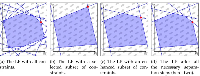
(a) The LP with all con-straints.
x2
x1
(b) The LP with a se-lected subset of con-straints.
x2
x1
(c) The LP with an en-hanced subset of con-straints.
x2
x1
(d) The LP after all the necessary separa-tion steps (here: two).
Figure 3: A geometric interpretation of an LP with two variablesx1, x2∈R(constraints presented as blue lines, objective function presented as gray arrows) and its solution (red). While (a) depicts the complete LP and an optimal solution, (b) to (d) show the advantages of using a separation algorithm: Starting with only a subset of constraints (b) we extend the LP with constraints which are violated by the solution to the current LP (c) as long as we can find any (see Figure 4). When the separation algorithm cannot find any violations (d) the current solution is valid and optimal with respect to the complete LP of the original model.
returns
Select a subsetC0 ⊆ C
of all of the problem’s constraints
Compute an optimal solution to the LP with constraint setC0
Does the solution s to
the LP satisfy all of the constraints ofCas well? Enhance C0 by a
vio-lated constraint inC
yes no
Figure 4: The way from Figure 3(b) to (d) as a diagram; the separation algorithm leads to a point of diversion depending on whether a violated constraint exists.
solution, augmenting the model, and resuming the optimization process) can be done via interfaces specified in the programming libraries of solvers like CPLEX and Gurobi. As the most simple iterative approach, this approach finally yields a globally optimal solution. Examples for the application of this method in computational cartography are presented by Haunert and Wolff [35] and Nöllenburg and Wolff [53].
therefore, may take very long. Instead of inspecting incumbent solutions for constraint vi-olation, we inspect optimal solutions ofLP relaxations—in the LP relaxation corresponding to a model the variables are allowed to take fractional values, which makes the problem less complex, even efficiently solvable [40]. Most ILP solvers begin with solving the LP relaxation of the given model to find a lower bound (or upper bound in case of a maxi-mization problem) of the objective function, usually by applying a variant of the simplex algorithm [16], which is fast in practice. Furthermore, during the optimization process, most solvers also solve LP relaxations for sub-instances (i.e., branch-and-bound nodes) in which the values of some variables are fixed. In any case, we test whether a solution of an LP relaxation of the current model satisfies all constraints of the original model. More precisely, we use aseparation algorithm, that is, an algorithm that either asserts that all con-straints are satisfied or yields a violated constraint, with which we then augment the model (see Figures 3 and 4). For the Traveling Salesperson Problem1, for example, this approach outperforms other ILP approaches [56]. In comparison to the previous approach based on incumbent solutions, one avoids an extensive exploration of the branch-and-bound tree. On the other hand, designing a separation algorithm can be a non-trivial task. If the con-straints are of a certain type, the separation step can be done efficiently (in particular, with-out explicitly testing all inequalities), for example by computing a maximum flow in an appropriately defined graph. Carvajal et al. [10] deal with forest planning models using this method. In Section 4 we exemplify this approach in detail for area aggregation.
4
A new method for area aggregation using cutting planes
In Section 2 we have modeled all aspects of the problem that we aim to solve. That is, we consider Objective (1) with the assignment costs in Equation (11) and the definition of the distanceδin Equation (12). We minimize this objective subject to Constraints (2)–(5) and constraints ensuring contiguity. Obviously, we could ensure contiguity with Constraints (6) and (7), but in this section we introduce an alternative formulation that we use with our cutting-plane method. An advantage of this formulation is that we get along with the binary variablesxc,vand without the additional variablesy(u,v)c .
Instead of setting up the model completely, we let the solver begin with the basic ILP from Section 2.1. When the solution to the LP relaxation in a branch-and-bound node is found, we intervene and check whether some of the not yet added contiguity constraints presented in the following are violated and add at least one of them in that eventuality.
With the following constraints we ensure contiguity. They are inspired by the work of Carvajal et al. [10] and Drexl and Haase [18], where they were set up in order to solve different problems: forest planning and sales territory alignment. The algorithm of Carvajal et al. solves a problem asking for the selection of a single output region and is therefore not directly applicable to the area aggregation problem. Drexl and Haase deal with districting but add violated constraints based not on the solution to the LP relaxation in a branch-and-bound node but to an optimal solution to the current model. Afterwards, they run experiments to calculate only upper and lower bounds for larger instances, but no optimal solutions. We do not only present these constraints in combination but also emphasize the
1Dealing with the Traveling Salesperson Problem means determining a shortest path visiting every city of a
c
v
c
v
c
v
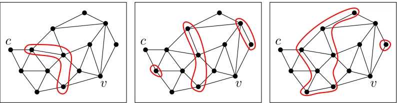
Figure 5: An example of an adjacency graphGwith various(c, v)-separators (red): Every path from
vtoccontains at least one vertex of the respective separator.
advantages of cutting-plane methods. Furthermore, we contribute an ILP formulation for area aggregation.
4.1
Constraints completing the ILP formulation
In the following, we present two different kinds of constraints. While combining the basic ILP from Section 2.1 with the constraints presented in Section 4.1.1 is necessary and suffi-cient for area aggregation, the constraints in Section 4.1.2 work in a supporting way. These supportive constraints mainly enforce the minimum-weight constraints (Constraint (4)) in a more determined manner.
4.1.1 Contiguity constraints based on vertex separators
Letc, v∈V be two arbitrary areas. In the following we considercthe center of a region and the possibility of assigningvto this region, which is represented with the binary variable
xc,v.
Furthermore, letSc,v ⊆ 2V be the set of all (c, v)-separators in G, where a set S ⊆ V \ {c, v} is called a(c, v)-separator if every path fromc to v inGcontains at least one vertex inS(see Figure 5). Ifvis allocated to the region with centerc, then—for the sake of contiguity—for each(c, v)-separatorS ∈ Sc,vat least one area ofS has to be allocated to
this region as well. In linear terms this condition is expressed as follows:
X
u∈S
xc,u≥xc,v for eachS∈Sc,v, c, v∈V. (13)
If c = v or {c, v} ∈ E, that is, areas c and v are identical or adjacent, the set of (c, v )-separatorsSc,vis empty. Consequently, there is no constraint described in Formula (13) for
these cases. In general, the number of separators is inO(2|V|).
fromctov, it also contains a vertex of pathpand thus an area of the region in question. Consequently, the inequalities from Constraint (13) are fulfilled. Now, let us assume that a regionR ⊆ V is not contiguous, i.e.,R consists of at least two connected components. Thus, it is possible to take a look at the region’s centercand an areavcontained in another connected component thanc. Then the setV \Ris a (c, v)-separator and the inequality from Constraint (13) is violated forS =V \R∈Sc,v.
4.1.2 Supportive constraints inspired by the minimum-weight requirement
If a separatorS ∈ Sc,v has certain properties, we define another constraint: sinceS is a
(c, v)-separator, the setV \Sconsists of at least two connected components—one of which containscand one of which containsv. LetC(S, c)be the connected component inV \S
containing c. If the total weight of C(S, c), that is P
u∈C(S,c)w(u), does not exceed the
minimum weightwmindemanded for a resulting region, then every region with centerc
has to contain at least one area of the separatorS. Or stated as a linear inequality:
X
u∈S
xc,u≥xc,c for eachS∈Sc,vwith
X
u∈C(S,c)
w(u)< wmin, c, v∈V (14)
Again, the inequality is always fulfilled forxc,c = 0. Only ifxc,c = 1(i.e.,cis declared a
center) the allocation of at least one area in the respective separator is required.
Constraint (14) alone does not suffice to achieve contiguity. When combining it with Constraint (13), however, it acts in a supportive manner. To see why, we contrast the con-tiguity constraint (Constraint (13)) with the supportive constraint (Constraint (14)). We observe that they only differ with respect to their right-hand sides, which arexc,v and xc,c, respectively. Constraint (3) ensures xc,c ≥ xc,v and, thus, Constraint (14) is at least
as restrictive as Constraint (13) for anyv ∈ V. That is, every solution to an LP relaxation considering Constraints (3) and (14) fulfills Constraint (13). However, the solution to an LP relaxation considering Constraints (3) and (13) cannot give this guarantee with respect to Constraint (14). Transferring this observation to Figure 3, we note that a more restrictive constraint cuts away more parts of the solution polytope (marked as a blue region in the figures). This results in a better performance of solvers based on branch and bound [52].
4.2
Adding the constraints
As described in Section 3, the ILP is built up step by step. In this section, we describe a separation algorithm, that is, an algorithm that allows us to find at least one violated conti-guity constraint if there exists any; see Section 4.2.1. Then, we show how such a conticonti-guity constraint may also provide a supportive constraint; see Section 4.2.2. Afterward, in Sec-tion 4.2.3, we discuss how to speed up the computaSec-tion by restricting the search for violated constraints, and we argue why this does not harm the correctness. Finally, in Section 4.2.4, we present another method that may find additional violated constraints without much computational overhead.
A pseudocode formulation of these algorithms can be found in Section Appendix B.
4.2.1 Finding violated contiguity constraints using minimum-weight vertex separators
If we assume that the integrality constraintsxc,v ∈ {0,1}are satisfied for all variables (see
c
v
1
1
1
1
0
0
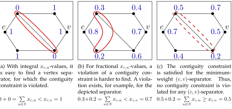
(a) With integral xc,u-values, it is easy to find a vertex sepa-rator, for which the contiguity constraint is violated.
0 + 0 = P
u∈S
xc,u< xc,v= 1
c
v
0
.
4
0
.
6
0
.
7
0
.
8
0
.
2
0
.
3
(b) For fractionalxc,u-values, a violation of a contiguity con-straint is harder to find. A viola-tion exists, for example, for the depicted separator.
0.3+0.2 = P
u∈S
xc,u< xc,v= 0.7
c
v
0
.
7
0
.
4
0
.
5
0
.
7
0
.
2
0
.
5
(c) The contiguity constraint is satisfied for the minimum-weight (c, v)-separator. Thus, no contiguity constraint is vio-lated for any(c, v)-separator.
0.5+0.2 = P
u∈S
xc,u≥xc,v= 0.5 Figure 6: In this example with fixedc, v∈V, we examine the search for a(c, v)-separator, for which the contiguity constraint (Constraint (13)) is violated. For a vertexu ∈ V, we consider the value
xc,u from the solution of an LP relaxation as its vertex weight (blue). It depends on these values whether a violation of a contiguity constraint exists. Separators which are interesting in this context are indicated in red.
fixed centerc, we could consider the subgraph ofGinduced by all nodesvwithxc,v= 1. Ifc
and a nodevlie in different connected components of this graph, a violation of a contiguity constraint exists. However, since we want to find constraints in a preliminary stage of the solution (i.e., in the solution of the LP relaxation of the ILP), we need to deal with variables of fractional values (see Figure 6(b)).
To find contiguity constraints that are violated by the solution to the current LP re-laxation, we proceed as follows (see also Algorithm 1 in Section Appendix B): taking a closer look at Constraint (13), we observe that separators providing a smaller sum on the constraint’s left-hand side are more likely to implicate a violation of the corresponding con-straint, since the right-hand side does not depend on the choice of the separator. For every potential centerc, we therefore take for everyv∈V the valuexc,vof the current solution as
the weight ofvinGand focus onminimum-weight(c, v)-separators afterward—in Section Appendix A we describe how to compute minimum-weight vertex separators by using minimum edge cut algorithms [13, 21, 26]. The reason why this is effective is the following: if the inequality from Constraint (13) is violated for an arbitrary(c, v)-separatorS, it is also violated for a minimum-weight(c, v)-separatorS∗ sincexc,c > Pu∈Sxc,u ≥ Pu∈S∗xc,u
holds in that case. Thus, for specificc, v∈V, looking at a minimum-weight(c, v)-separator guarantees to notice a violation if there is one (see Figure 6(c)). In particular, computing and examining minimum-weight (c, v)-separators for every potential center c ∈ V and everyv∈V \ {c}solves the separation problem.
4.2.2 Finding supportive constraints
c
v
(a)
c
v
(b)
Figure 7: The(c, v)-separator (red) divides the graph into at least two connected components. The component ofc(dashed, blue) in (b) is more likely to offer a Constraint (14) than the one in (a).
connected components in G. If one of these components forms a region with less than the minimum weight, the corresponding separator offers Constraint (14) for any potential center in that component. Therefore, we check for every area in the connected component ofc whether the respective Constraint (14) is violated for this area as a center. If that is the case, we add the violated constraint to the model. This means we compute a separator principally for a certain centercbut also use it to set up constraints independent fromc.
The algorithm from Section 4.2.1 yields a minimum-weight(c, v)-separator. Such a sep-arator is not unique. Among the minimum-weight(c, v)-separators we prefer those which are closer toc (see Figure 7). The reason why we prefer separators closer to c is Con-straint (14): That way, it is more likely to detect violations of ConCon-straint (14) and conse-quently more likely to add a supportive constraint. In order to find the minimum-weight (c, v)-separator closest toc we use the fact that our algorithm is based on the search for a minimum edge cut. Here, common algorithms follow the same scheme and return the minimum edge cut closest to a certain vertex [13].
4.2.3 Restricting the search for violated constraints
A straightforward implementation of the algorithm described in Section 4.2.1 implicates the computation of a quadratic number of vertex separators every time an LP relaxation is solved optimally. In order to reduce this number, we make restrictions described in the following.
We read the value of a variable xc,v for arbitraryc, v ∈ V as the tendency ofv to be
allocated toc. With regard to Constraint (2), we see that, for a fixedv ∈ V, the average value of the variablesxc,v is |V1|. Therefore, we interpretxc,v ≥ |V1| as an indicator that
allocatingvtoc(or, in the casev=c, declaringva center) is—for the moment—considered reasonable. Conversely, a value less than 1
|V| implicates that an allocation to a different
center is preferable. Hence, we impose the following restrictions on the method presented in Sections 4.2.1 and 4.2.2:
• We compute minimum-weight(c, v)-separators only for areasvwithxc,v≥|V1|. • We take centerscwith xc,c < |V1| only into consideration if no violation is detected
• We add a supportive constraint (Constraint (14)) only for areasv in the connected component (not fulfilling the minimum-size requirement) of the examined center for whichxv,v≥|V1|holds.
Although we fail to notice violations of the inequality from Constraint (13) for areas withxc,v< |V1|and, thus, to solve the separation problem properly, this fact does not pose
a risk to finding a contiguous solution. As we handle these violations in a branch-and-bound node, the solver goes on branching and branch-and-bounding in the node’s sub-instances. It continues until either an integral solution is found or the problem becomes infeasible. If a sub-instance is infeasible, there is no need to worry about whether the number of added constraints is too small. In case of an integral solution, there are two possible scenarios for each potential region with centerc: eitherxc,c = 0and with itxc,v ≤ xc,c = 0 for every v∈V (see Constraint (3)), i.e., the region is not considered in the solution and therefore in no need of a validation of contiguity. Orxc,c = 1≥ |V1|, which results in a verification of
the region’s contiguity and implies that we find violations if existing.
4.2.4 Finding violated contiguity constraints using connected components
For the following method of finding a useful vertex separator (see also Algorithm 2 in Section Appendix B), we interpret for every probable centerc(i.e.,xc,c ≥ |V1|) the values
of the variablesxc,v forv ∈V as described in Section 4.2.3, only stricter: ifxc,v ≥ |V1|, we
considervallocated to the region with centerc, otherwise we do not. Therefore, we take a look at
V0 =nv∈V xc,v≥
1
|V| o
and to the subgraph ofGinduced byV0. In this subgraph we are able to detect connected components of the areas tending to be allocated to c. For every connected component
U ⊆V0⊆V withc /∈U, we examine the set of adjacent areas inV, that is
BU :=
w∈V \U ∃u∈U :{u, w} ∈E , (15)
and take it as a vertex separator. Subsequently, we add a Constraint (13) for everyu∈ U
(and c). This way we have a good chance of finding additional violated contiguity con-straints without much computational overhead.
5
Results and discussion
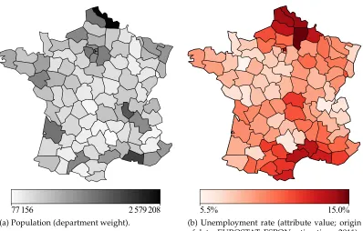
77 156 2 579 208
(a) Population (department weight).
5.5% 15.0%
(b) Unemployment rate (attribute value; origin of data: EUROSTAT, ESPON estimations, 2011).
Figure 8: input data for statistical aggregation of France’s departments
take the population of a department [23] (see Figure 8(a)) instead of its area as the depart-ment’s weight. This means we compare the methods described in Sections 2.2 and 4 on the third level administrative subdivision of a major European country. We do not only com-pare the effects ofα, the factor weighting the cost functionsfrecolor and fnon-compactin the objective function, on the result and the computation time, but also examine the influence of the choice ofwmin, the minimum weight required of a region in the output.
As attribute domain,Γ = [0,1]is given and we writeγv ∈ Γ for the attribute value,
i.e., unemployment rate, of an areav ∈V. According to Section 2.3, we defineδ(γ1, γ2) = |γ1−γ2|for arbitraryγ1, γ2∈Γas the cost for recoloring. The cost for non-compactness is
defined through the Euclidean distancedbetween centroids. Observing Equations (1) and (8)–(10) we get the following overall cost function as the objective function:
X
c∈V
X
v∈V\{c}
w(v)·α·d(c, v) + (1−α)·δ(γc, γv)
·xc,v (16)
As for the weighting factorα, we make the following choice: withα∈ {0,1}we want to present the extreme solutions. Forα= 1we receive compact regions of a certain weight ignoring any statistical similarities between the areas. Forα = 0we see a solution with least recoloring costs but consisting of regions of mostly unconventional shape. According to the experiments that we present in this section, a weighting factor ofα= 2·10−5 still
yields almost optimally compact shapes andα= 1.25·10−6almost optimally homogeneous
In our experiments, we setwmin to 5 %and 10 %respectively of the total population
of continental France. With this setting, we end up with a partitioning into a number of larger regions which is approximately at the same scale as the actual NUTS-2 subdivision of continental France, which consists of 12 regions.
Figure 9 α tcut tflow tflow/tcut #out
(a) 1 30 s 497 s 16.6 18
(b) 2.0 ·10−5 21 s 502 s 23.9 18
(c) 5.0 ·10−6 50 s 14 229 s≈4.0 h 284.6 17
(d) 2.5 ·10−6 100 s >5 d >4 320.0 16
(e) 1.25·10−6 451 s >5 d > 957.9 16
(f) 0 18 413 s≈5.1 h >5 d > 23.4 14
(1) Running times for the experiments with minimum weightwmin= 201 Pv∈Vw(v).
Figure 10 α tcut tflow tflow/tcut #out
(a) 1 20 s 35 s 1.8 9
(b) 2.0 ·10−5 59 s 267 s 4.5 9
(c) 5.0 ·10−6 194 s 14 464 s≈4.0 h 74.6 9
(d) 2.5 ·10−6 495 s >5 d > 872.7 9
(e) 1.25·10−6 86 981 s≈1 d >5 d > 4.9 9
(f) 0 >5 d >5 d — 92
(2) Running times for the experiments with minimum weightwmin= 101 Pv∈Vw(v).
Tables (1) and (2): These tables provide information about the running times in seconds (s), hours (h) or days (d) for the corresponding experiments with different minimum weights (see Equation (4)). Experiments were aborted after five days if no optimal solution was found; this is indicated with “>5
d.” The first column refers to the visual presentation of the result. The second column denotes the
α-value used in this experiment (see Equation (16)). In the column marked withtcutone can find the running times of our approach described in Section 4, in the column marked withtflowthe times of the state-of-the-art approach of Section 2. The fifth column compares those values by giving the ratio
tflow/tcut. Finally, the column marked with#outgives additional information about the structure of the result by providing the number of resulting regions.
Considering the results in Tables (1) and (2), it comes to attention that our cutting-plane approach outperforms the flow model in every instance. In our experiments, the flow MILP is competitive only in the situation wherewminis10 %of the total population andα= 1.
In every other case, our ILP is many times faster, as the fifth column of each table indicates. With αdeclining, i.e., focusing on reducing frecolor, the advantages of the cutting-plane formulation become clearer since the problem becomes harder to solve. This is caused by the fact that focusing on compactness supports contiguity: a compact region is more likely to be contiguous than a region of areas with similar attributes.
In particular, the three last rows of each table deserve our special attention. For both settings of wmin, the solver is not able to return a result using the flow model for α ≤
2.5·10−6. Leaving the instance withα= 0,wmin = 101 Pv∈V w(v)out of account, each of
2Since the calculations are incomplete for both the flow model and the cutting-plane approach, the result
Aveyron
(a)α= 1 (b)α= 2.0·10−5
(c)α= 5.0·10−6 (d)α= 2.5·10−6
(e)α= 1.25·10−6 (f)α= 0
(a)α= 1 (b)α= 2.0·10−5
(c)α= 5.0·10−6 (d)α= 2.5·10−6(same result as (e))
(e)α= 1.25·10−6(same result as (d)) (f)α= 0(interim result2)
these instances is solvable with the cutting-plane algorithm. For three of these instances, the solver returns an optimal solution within a few minutes.
Considering the output in detail, we find that the noticeable higher unemployment rates in northern and southern France (former Nord-Pas-de-Calais and on the Mediterranean coast) are identified and aggregated in every example where similarity is considered (i.e.,
α6= 1). In general, for most of the departments, the resulting color (unemployment rate) is close to the input. Nevertheless, one also notices larger differences between input and out-put coloring for various departments. This phenomenon occurs especially forα= 1, but also in other cases. Forα6= 1, however, this only causes minor changes since these depart-ments have a comparatively small population (see Figure 8(a)) and consequently contribute only little cost. Take, for example, Aveyron, a department in south-central France (see Fig-ure 9(a)) with one of the lowest unemployment rates of all departments. For bothα = 1 andα = 0it has undergone seemingly expensive recoloring. Considering the objective, this makes sense as less than0.5 %of France’s total population lives in Aveyron.
Another negative aspect is the fact that parts of some of the resulting regions are very narrow. Understandably, this occurs especially forα = 0, where resulting regions reach diagonally from one border to another, e.g., in both Figures 9(f) and 10(f) the region con-taining the department in the very south-west (Pyrénées-Atlantiques). Forα6= 0this phe-nomenon occurs less distinctly. A problem that arises independent ofαis bottlenecks. A bottleneck is a very narrow part of a region connecting two larger parts. In order to resolve this, one has to manipulate the input data or rather its interpretation. Building the adja-cency graphG, we consider departments adjacent as soon as they share a boundary. When dealing with a map of France’s departments, we have to handle several pairs of depart-ments sharing a borderline of less than10 km. Without adjusting the adjacency rule, we see results with constellations such as in Figures 9(e) and 9(f), where a region bordering the Mediterranean Sea (marked with an arrow in the south-east) even seems to consist of two components. Here, the departments Var and Vaucluse share less than1 kmof borderline.
Figure 11 gives us additional arguments to disqualifyα = 0orα = 1as reasonable weight factors. Let us take a look at the situation forwminequaling5 %of the total
popula-tion (i.e., Figure 11(a)). Asα= 0(here: (f)) results in an optimal solution with respect to the cost for recoloring, these costs are higher for every other value ofα. But forα= 1.25·10−6 (here: (e)), recoloring is only approximately1.2 %more expensive (47.06 %versus47.65 % of the maximum value) whereas the cost for non-compactness decreases by32.4 %. The situation is the same for the other value ofwminand similar with regard to the cost for
non-compactness. Also, this argument supports our choice forα≈10−5. In this range, we get
near-optimal results for either cost without unreasonable expenses for the other.
6
Conclusion
frecolor
fnon-compact
0.4 0.5 0.5
0.75 0.75
1 1
(f)
(e)
(d) (c)
(b) (a)
(a) Comparison for wmin equaling 5 % of France’s total population, see Table (1) and Fig-ure 9; absolute maximum values are8.0·1012 (non-compactness) and6.4·107(recoloring).
frecolor
fnon-compact
0.4 0.5 0.5
0.75 0.75
1 1
(f)2
(d),(e) (c)
(b) (a)
(b) Comparison for wmin equaling 10 % of France’s total population, see Table (2) and Fig-ure 10; absolute maximum values are9.2·1012 (non-compactness) and8.4·107(recoloring). Figure 11: Costs for non-compactness and recoloring as a percentage of the maximum occurring cost; as100 %of costs for non-compactness we take those arising while minimizing the cost for recoloring (i.e.,α= 0) and vice versa.
the largest in the European Union—the solver returns no optimal solution within five days. This problem occurs even forα= 1, i.e., focusing on compactness only.
Nevertheless, our approach offers unprecedented opportunities. Five of the instances from our experiments are set up too hard to be solved with the flow MILP within five days but are solvable with the cutting-plane algorithm within one day. In particular, the solver is capable to find an optimal solution for each of these settings which consider not only recoloring but also compactness, i.e.,α6= 0. Moreover, three of these four cases are solved within only a few minutes. Due to these positive results, we argue that we have increased the range of problem instances that can be solved with proof of optimality such that it includes use cases that are of relevance. In particular, we consider it promising to use our method to produce benchmark solutions and to compare such solutions with solutions of efficient heuristic methods. Such a comparison may help to decide whether or not a heuristic is a justifiable choice. Therefore, we think that both exact and heuristic methods for area aggregation can complement each other and will play their roles in the future.
In future work, we plan to support the ILP solver by calling heuristics during branching or in order to generate an initial solution. Furthermore, we consider it promising to apply our cutting-plane approach to thep-region problem [20], in which the number of output regions is prescribed.
References
[2] ALTMAN, M. The computational complexity of automated redistricting: Is automa-tion the answer? Rutgers Computer and Law Technology Journal 23, 1 (1997), 81– 142. http://heinonline.org/HOL/Page?handle=hein.journals/rutcomt23&g sent=1& id=87&collection=journals.
[3] ÁLVAREZ-MIRANDA, E., LJUBI ´C, I., AND MUTZEL, P. The maximum weight con-nected subgraph problem. InFacets of Combinatorial Optimization: Festschrift for Martin Grötschel, M. Jünger and G. Reinelt, Eds. Springer, Berlin, Germany, 2013, pp. 245–270. doi:10.1007/978-3-642-38189-8_11.
[4] BADER, M., BARRAULT, M.,ANDWEIBEL, R. Building displacement over a ductile truss. International Journal of Geographical Information Science 19, 8-9 (2005), 915–936. doi:10.1080/13658810500161237.
[5] BELLMORE, M.,ANDNEMHAUSER, G. L. The traveling salesman problem: A survey. Operations Research 16, 3 (1968), 538–558. doi:10.1287/opre.16.3.538.
[6] BERTIN, J. Semiology of Graphics: Diagrams, Networks, Maps, 1st ed. The University of Wisconsin Press, 1983.
[7] BOZKAYA, B., ERKUT, E., AND LAPORTE, G. A tabu search heuristic and adaptive
memory procedure for political districting.European Journal of Operational Research 144 (2003), 12–26. doi:10.1016/S0377-2217(01)00380-0.
[8] BRASSEL, K. E.,ANDWEIBEL, R. A review and conceptual framework of automated
map generalization.International Journal of Geographical Information Systems 2, 3 (1988), 229–244. doi:10.1080/02693798808927898.
[9] CARO, F., SHIRABE, T., GUIGNARD, M., ANDWEINTRAUB, A. School redistricting:
Embedding GIS tools with integer programming. Journal of the Operational Research Society 55, 8 (2004), 836–849. doi:10.1057/palgrave.jors.2601729.
[10] CARVAJAL, R., CONSTANTINO, M., GOYCOOLEA, M., VIELMA, J. P., AND WEIN -TRAUB, A. Imposing connectivity constraints in forest planning models. Operations Research 61, 4 (2013), 824–836. doi:10.1287/opre.2013.1183.
[11] CASADO-DÍAZ, J. M. Local labour market areas in Spain: A case study. Regional Studies 34, 9 (2000), 843–856. doi:10.1080/00343400020002976.
[12] CHRISTOFIDES, N. The vehicle routing problem. Revue française d’automatique, d’informatique et de recherche opérationnelle. Recherche opérationnelle 10, 1 (1976), 55–70. doi:10.1051/ro/197610V100551.
[13] CORMEN, T., LEISERSON, C., RIVEST, R.,AND STEIN, C. Introduction To Algorithms. MIT Press, 1990.
[14] COVA, T. J., AND CHURCH, R. L. Contiguity constraints for single-region site search problems. Geographical Analysis 32, 4 (Sep 2010), 306–329. doi:10.1111/j.1538-4632.2000.tb00430.x.
[16] DANTZIG, G. B. Linear Programming and Extensions. Princeton University Press, 1963.
[17] DEBERG, M.,VANKREVELD, M.,ANDSCHIRRA, S. Topologically correct subdivision simplification using the bandwidth criterion. Cartography and Geographic Information Systems 25, 4 (1998), 243–257. doi:10.1559/152304098782383007.
[18] DREXL, A.,ANDHAASE, K. Fast approximation methods for sales force deployment. Management Science 45, 10 (1999), 1307–1323. doi:10.1287/mnsc.45.10.1307.
[19] DUQUE, J. C., ANSELIN, L., ANDREY, S. J. The max-p-regions problem. Journal of Regional Science 52, 3 (Aug 2012), 397–419. doi:10.1111/j.1467-9787.2011.00743.x.
[20] DUQUE, J. C., CHURCH, R. L.,ANDMIDDLETON, R. S. The p-regions problem. Geo-graphical Analysis 43, 1 (2011), 104–126. doi:10.1111/j.1538-4632.2010.00810.x.
[21] EDMONDS, J., AND KARP, R. M. Theoretical improvements in algorithmic
ef-ficiency for network flow problems. Journal of the ACM 19, 2 (1972), 248–264. doi:10.1145/321694.321699.
[22] EUROPEANOBSERVATIONNETWORK FORTERRITORIALDEVELOPMENT ANDCOHE
-SION. European Regions 2010: Economic Welfare and Unemployment, 2011. http:// www.espon.eu/main/Menu Publications/Menu MapsOfTheMonth/map1103.html.
[23] EUROSTAT. Population by single year of age and NUTS 3 region, 2015. http://appsso. eurostat.ec.europa.eu/nui/show.do?dataset=cens 11ag r3&lang=en.
[24] FISCHETTI, M., AND MONACI, M. Cutting plane versus compact formulations for uncertain (integer) linear programs. Mathematical Programming Computation 4, 3 (Sep 2012), 239–273. doi:10.1007/s12532-012-0039-y.
[25] FLÓREZ-REVUELTA, F., CASADO-DÍAZ, J. M., AND MARTÍNEZ-BERNABEU, L. An evolutionary approach to the delineation of functional areas based on travel-to-work flows. International Journal of Automation and Computing 5, 1 (2008), 10–21. doi:10.1007/s11633-008-0010-6.
[26] FORD, L. R., AND FULKERSON, D. R. Maximal flow through a network. Journal canadien de mathématiques 8, 0 (1956), 399–404. doi:10.4153/CJM-1956-045-5.
[27] GALANDA, M. Automated Polygon Generalization in a Multi Agent System. dissertation, University of Zurich, Switzerland, 2003.
[28] GAREY, M. R.,ANDJOHNSON, D. S.Computers and Intractability; A Guide to the Theory of NP-Completeness. W. H. Freeman & Co., San Francisco, 1990.
[29] GARFINKEL, R. S., AND NEMHAUSER, G. L. Optimal political districting by implicit enumeration techniques. Management Science 16, 8 (1970), B–495–B–508. doi:10.1287/mnsc.16.8.B495.
[31] GUROBIOPTIMIZATION, INC. Gurobi optimizer reference manual, 2015. http://www. gurobi.com.
[32] HARRIE, L., AND WEIBEL, R. Modelling the overall process of generalisation.
In Generalisation of Geographic Information: Cartographic Modelling and Applications, W. Mackaness, A. Ruas, and L. T. Sarjakoski, Eds. Elsevier, 2007, ch. 4, pp. 67–87. doi:10.1016/B978-008045374-3/50006-5.
[33] HAUNERT, J.-H. Aggregation in Map Generalization by Combinatorial Optimization. Dis-sertation, Leibniz Universität Hannover, Germany, 2008.
[34] HAUNERT, J.-H.,ANDWOLFF, A. Area aggregation in map generalisation by mixed-integer programming. International Journal of Geographical Information Science 24, 12 (2010), 1871–1897. doi:10.1080/13658810903401008.
[35] HAUNERT, J.-H., AND WOLFF, A. Optimal and topologically safe simplifi-cation of building footprints. In Proc. 18th SIGSPATIAL International Confer-ence on Advances in Geographic Information Systems (ACMGIS) (2010), pp. 192–201. doi:10.1145/1869790.1869819.
[36] HESS, S. W., AND SAMUELS, S. A. Experiences with a sales districting model: Criteria and implementation. Management Science 18, 4, Part II (1971), 41–54. doi:10.1287/mnsc.18.4.P41.
[37] HESS, S. W., WEAVER, J. B., SIEGFELDT, H. J., WHELAN, J. N., AND ZITLAU, P. A. Nonpartisan political redistricting by computer. Operations Research 13, 6 (1965), 998– 1006. doi:10.1287/opre.13.6.998.
[38] HOJATI, M. Optimal political districting.Computers & Operations Research 23, 12 (1996), 1147–1161. doi:10.1016/S0305-0548(96)00029-9.
[39] JÜNGER, M., REINELT, G., ANDTHIENEL, S. Practical problem solving with cutting
plane algorithms in combinatorial optimization. Dimacs Series in Discrete Mathemat-ics and Theoretical Computer Science 20 (1995), 111–152. http://e-archive.informatik. uni-koeln.de/156/.
[40] KARMARKAR, N. A new polynomial-time algorithm for linear programming. Combi-natorica 4, 4 (1984), 373–395. doi:10.1007/BF02579150.
[41] KWAN, M.-P., CASAS, I., ANDSCHMITZ, B. Protection of geoprivacy and accuracy of spatial information: How effective are geographical masks? Cartographica: The International Journal for Geographic Information and Geovisualization 39, 2 (2004), 15–28. doi:10.3138/X204-4223-57MK-8273.
[42] LAPORTE, G. The traveling salesman problem: An overview of exact and approx-imate algorithms. European Journal of Operational Research 59, 2 (Jun 1992), 231–247. doi:10.1016/0377-2217(92)90138-Y.
[44] LI, W., GOODCHILD, M. F., AND CHURCH, R. L. An efficient measure of com-pactness for two-dimensional shapes and its application in regionalization problems. International Journal of Geographical Information Science 27, 6 (Jun 2013), 1227–1250. doi:10.1080/13658816.2012.752093.
[45] LIGMANN-ZIELINSKA, A., CHURCH, R. L., AND JANKOWSKI, P. Spatial opti-mization as a generative technique for sustainable multiobjective land-use alloca-tion. International Journal of Geographical Information Science 22, 6 (2008), 601–622. doi:10.1080/13658810701587495.
[46] LINDEROTH, J. T., AND RALPHS, T. K. Noncommercial software for mixed-integer
linear programming. Integer Programming: Theory and Practice 3 (2005), 253–303. doi:10.1201/9781420039597.ch10.
[47] MACEACHREN, A. M. Compactness of geographic shape: Comparison and evalu-ation of measures. Geografiska Annaler. Series B, Human Geography 67, 1 (1985), 53. doi:10.2307/490799.
[48] MACKANESS, W. A., AND BEARD, M. K. Use of graph theory to support map generalization. Cartography and Geographic Information Systems 20 (1993), 210–221. doi:10.1559/152304093782637479.
[49] MEHROTRA, A., JOHNSON, E. L., AND NEMHAUSER, G. L. An optimization
based heuristic for political districting. Management Science 44, 8 (1998), 1100–1114. doi:10.1287/mnsc.44.8.1100.
[50] MUYLDERMANS, L., CATTRYSSE, D., VANOUDHEUSDEN, D., ANDLOTAN, T. Dis-tricting for salt spreading operations. European Journal of Operational Research 139, 3 (2002), 521–532. doi:10.1016/S0377-2217(01)00184-9.
[51] NAVEH, B. JGraphT, 2016. http://jgrapht.org/.
[52] NEMHAUSER, G. L., AND WOLSEY, L. Integer and Combinatorial Optimization. John
Wiley & Sons, Inc., Hoboken, NJ, USA, 1988. doi:10.1002/9781118627372.
[53] NÖLLENBURG, M.,ANDWOLFF, A. Drawing and labeling high-quality metro maps by mixed-integer programming.IEEE transactions on visualization and computer graphics 17, 5 (2010), 626–641. doi:10.1109/TVCG.2010.81.
[54] OPENSHAW, S. The modifiable areal unit problem. Concepts and Techniques in Modern Geography 38(1984), 1–41.
[55] PAPPS, K. L.,ANDNEWELL, J. O. Identifying functional labour market areas in new zealand: A reconnaissance study using travel-to-work data.IZA Discussion Papers 443, 1 (2002). http://ftp.iza.org/dp443.pdf.
[56] PATAKI, G. Teaching integer programming formulations using the traveling salesman problem.SIAM Review 45, 1 (2003), 116–123. doi:10.1137/S00361445023685.
[58] RICCA, F., SCOZZARI, A., AND SIMEONE, B. Political districting: From classi-cal models to recent approaches. Annals of Operations Research 204(2013), 271–299. doi:10.1007/s10479-012-1267-2.
[59] SESTER, M. Optimization approaches for generalization and data abstraction. International Journal of Geographical Information Science 19, 8–9 (2005), 871–897. doi:10.1080/13658810500161179.
[60] SHIRABE, T. Classification of spatial properties for spatial allocation modeling. GeoIn-formatica 9, 3 (2005), 269–287. doi:10.1007/s10707-005-1285-1.
[61] SHIRABE, T. A model of contiguity for spatial unit allocation.Geographical Analysis 37, 1 (2005), 2–16. doi:10.1111/j.1538-4632.2005.00605.x.
[62] SHIRABE, T. Districting modeling with exact contiguity constraints. Environment and Planning B: Planning and Design 36, 6 (2009), 1053–1066. doi:10.1068/b34104.
[63] SHIRABE, T., AND TOMLIN, C. D. Decomposing integer programming models for spatial allocation. InGeographic Information Science, M. J. Egenhofer and D. M. Mark, Eds. Springer, Berlin, Germany, 2002, ch. 21, pp. 300–312. doi:10.1007/3-540-45799-2_21.
[64] SMART, M. W. Labour market areas: Uses and definition.Progress in Planning 2(1974), 239–353. doi:10.1016/0305-9006(74)90008-7.
[65] VAN ROY, T. J., AND WOLSEY, L. A. Solving mixed integer programming problems using automatic reformulation. Operations Research 35, 1 (1987), 45–57. doi:10.1287/opre.35.1.45.
[66] WANG, Y., BUCHANAN, A., AND BUTENKO, S. On imposing connectivity con-straints in integer programs. Mathematical Programming 166, 1 (Nov 2017), 241–271. doi:10.1007/s10107-017-1117-8.
[67] WARE, J. M., JONES, C. B.,AND THOMAS, N. Automated map generalization with multiple operators: a simulated annealing approach. International Journal of Geograph-ical Information Science 17, 8 (2003), 743–769. doi:10.1080/13658810310001596085.
[68] WEIBEL, R. Generalization of spatial data: Principles and selected algorithms. In Algorithmic Foundations of Geographic Information Systems. Springer, Berlin, Germany, 1997, pp. 99–152. doi:10.1007/3-540-63818-0_5.
[69] WILLIAMS, J. C. A zero-one programming model for contiguous land acquisition. Geographical Analysis 34, 4 (2002), 330–349. doi:10.1111/j.1538-4632.2002.tb01093.x.
Appendix A
Minimum-weight vertex separators
For defining the constraints in Section 4.1.1 we use minimum-weight vertex separators. In this section we explain what these separators are and how to calculate them by using established minimum edge cut algorithms [13, 21, 26].
u v
z
e
G
c
(a) A quadrilateral as an explanatory graphG= (V, E). Here, we are looking for a minimum-weight(c, v)-separator.
˜
G
˜ c0 ˜ c1 ˜ v0 ˜ v1 ˜ z0 ˜ z1 ˜ ae 0 ˜ ae 1 ˜ ac ˜ av ˜ az ˜ u0 ˜ u1 ˜ au(b) The transformationG˜ = ( ˜V ,A˜) ofG; ele-ments inV˜andA˜induced byV are black, those inA˜induced byEare red.
˜
G
w(u)
w(z)
m m m m ˜ c1 ˜ v0 ˜ au ˜ az
(c) Blue arcs represent a maximum flow with corresponding weights from c˜1 () to ˜v0 (); sincemis a sufficiently large constant, the max-imum flow is w(u) +w(z), limited by arcs in-duced byV (here: the dotted arcs˜au, ˜az with weightsw(u),w(z)respectively).
u v
z
e
G
c
(d) Figure (c) finally provides a minimum-weight edge cut{˜au,˜az}. Transferring this result back toG, we get the wanted minimum-weight
(c, v)-separator{u, z}.
Figure 12: Computing a minimum-weight vertex separator.
follow-ing property: Every path inGfromctovcontains at least one vertex inS. Furthermore, any set with this property has at least the same weight asSwith respect tow.
Ifc=vor{c, v} ∈Ethen there exists no such vertex andS=∅. In every other case we make use of minimum(c, v)-cut algorithms and apply them to a modified graphG˜.
In order to use edge cut algorithms we need to transformGinto a directed graphG˜ = ( ˜V ,A˜)(see Figure 12(a) and (b)). Since only vertex weights are given and we want to use edge weights, we have to introduce two verticesv˜0,˜v1 ∈V˜ and an arca˜v = (˜v0,v˜1) ∈ A˜
for every v ∈ V with w˜(˜av) = w(v), where w˜: ˜A → R≥0 is an edge-weight function.
Furthermore, we replace every edgee ∈ E with two arcs ˜ae
0,˜ae1 ∈ A˜ going in opposite
directions to maintain the structure of the graph. With definingw˜(˜a0) = ˜w(˜a1) = m∈ R
withm >P
v∈V w(v)we complete the transformation.
Let A˜V =
˜
av
v∈V be the set of all arcs induced by V (in the example, A˜V = {˜ac,˜au,˜av,˜az}, see Figure 12(b)). As, in general, A˜V \ {˜ac,˜av} is a(c, v)-cut with weight
P
a∈A˜V\{˜au,˜av}w˜(a) less thanm = ˜w(˜a)for every ˜a ∈ ˜
A\A˜V we do not only know a
cut without any arcs induced byE, but also that any minimum-weight cut is a subset of ˜
AV \ {˜au,˜av}. Hence we are able to conclude from the computed minimum-weight cut to
a minimum-weight vertex separator.
Appendix B
Algorithms
In the following section we present the algorithms corresponding to the methods of adding constraints to the model which are described in Section 4.2. For both Algorithms 1 and 2, we use—in addition to the adjacency graphG= (V, E)—a matrix of ILP variables indexed in the same manner as throughout the article (x[c][v]corresponds toxc,v). As already
men-tioned, we only considerx-values exceeding a certain bound; in Section 4.2.3 we choose 1
|V|
which we use in these algorithms.
With Algorithm 1 we are able to find cuts using minimum vertex separators as de-scribed in Sections 4.2.1 and 4.2.2. Some parts of the algorithm need explanatory remarks:
• To find a vertex separator inG, we use aVertexSeparatorGenerator. That is an object of the classMinSourceSinkCutof the library JGraphT [51] applied to an auxiliary graph as described in Section Appendix A.
• The boolean variablehasAdditionalCutsguarantees a sufficiently neat solution of the separation problem. The search for vertex separators (and consequently additional constraints) continues until a cut is added to the current LP relaxation, but at least as long as the value of thex-variable of the center is greater or equal 1
|V|.
hasAdditional-Cutsis the output of Algorithm 1 and this output is an argument of Algorithm 2. In Algorithm 2, this boolean variable is used for the same purpose.
Algorithm 1:addVertexSeparatorCuts
Data:Adjacency graphG= (V, E),V sorted such thatv≥w⇔xv,v≥xw,wfor v, w∈V, Variable[ ][ ]x
Result:Cuts added by means of vertex separators (see Sections 4.2.1 and 4.2.2) 1 Gen←V e
![Figure 1: An example of area aggregation (see Haunert and Wolff [34]).](https://thumb-us.123doks.com/thumbv2/123dok_us/1156671.1617740/3.612.113.516.116.217/figure-example-area-aggregation-haunert-wolff.webp)