BIOINFORMATICS
Vol. 00 no. 00 Pages 1–7Gene Set Enrichment Analysis using Linear Models and
Diagnostics
Assaf P. Oron,
a
∗
Zhen Jiang and Robert Gentleman
a
a
Fred Hutchinson Cancer Research Center, 1100 Fairview Avenue North, Seattle, Washington
98109-1024, U.S.A.
ABSTRACT
Motivation: Gene-set enrichment analysis (GSEA) can be greatly enhanced by linear model (regression) diagnostic techniques. Diagnostics can be used to identify outlying or influential samples, and also to evaluate model fit and explore model expansion.
Results: We demonstrate this methodology on an adult acute lymphoblastic leukemia (ALL) dataset, using GSEA based on chromosome-band mapping of genes. Individual residuals, grouped or aggregated by chromosomal loci, indicate problematic samples and potential data-entry errors, and help identify hyperdiploidy as a factor playing a key role in expression for this dataset. Subsequent analysis pinpoints suspected DNA copy number abnormalities of specific samples and chromosomes (most prevalent are chromosomes X, 21 and 14), and also reveals significant expression differences between the hyperdiploid and diploid groups on other chromosomes (most prominently 19, 22, 3 and 13) - differences which are apparently not associated with copy number.
Availability: Software for the statistical tools demonstrated in this article is available as Bioconductor package GSEAlm.
Contact:[email protected],[email protected]
1 INTRODUCTION
Gene set enrichment analysis (GSEA, Mootha
et al.
, 2003;
Subramanian
et al.
, 2005) is an important new approach to
the analysis of gene expression data, and it has already been
extended and generalized in a number of ways (Tian
et al.
,
2005; Kim and Volsky, 2005; Jiang and Gentleman, 2007;
Hummel
et al.
, 2008). Expression analysis in general and
GSEA in particular can be viewed as a cascade of successive
data reductions: first, biochemical hybridization information
is reduced to a set of pixel images (typically one or two per
sample). Second, the images are pre-processed to produce
probe-level summaries, which are then further summarized to
a
G
×
n
matrix of normalized average expression estimates
(
G
genes,
n
samples). This matrix is then filtered to remove
∗to whom correspondence should be addressed
redundant probesets and genes identified as unexpressed or
otherwise uninformative (non-specific filtering). Next,
dataset-level differential expression statistics are calculated for each
gene. Finally, these statistics are used to calculate
gene-set-level statistics, which help identify differentially expressed or
otherwise interesting gene-sets. This data-reduction process is
essential. It helps bring the amount of information generated by
the microarray experiment down to a manageable level, while
retaining its core features. However, the quality of such massive
data reduction can and should be monitored. Monitoring the
last stages of this process is where linear model tools may prove
beneficial.
Several studies (e.g. Goeman
et al.
, 2004; Kim and Volsky,
2005; Kong
et al.
, 2006; Jiang and Gentleman, 2007; Hummel
et al.
, 2008) have demonstrated the potential of using a
linear model (regression) framework for GSEA. In particular,
with linear models one can adjust for important explanatory
covariates, such as sex and ER status for breast cancer. These
studies focus mostly on the use of linear models to evaluate
covariate effects upon gene-set expression,
averaged
over the
relevant genes and samples. This averaging aspect of linear
models is complemented by
diagnostics
, in particular residuals
– which examine the model’s adequacy in describing the
original data patterns, and also individual deviations from the
average effects. In this paper we demonstrate the application of
linear model diagnostics to GSEA.
2 METHODS
2.1 Linear Models and Diagnostics
A linear (regression) model assumes that the mean of the response variable has a linear relationship with the explanatory covariate(s). In gene-expression terminology, a simple generic model could be written as:
ygi=βg0+ p X
j=1
Xijβgj+²gi, (1)
•
ygi, g = 1, . . . G, i = 1, . . . nis the gene expression value ofgenegin samplei;
•
pis the number of explanatory covariates in the model;•
Xij is the value of thej-th covariate for thei-th sample. Fordichotomous covariates such as phenotype, one typically setsX
to zero or one (e.g.,NEGwill be zero andBCR/ABLone);
•
βgj is the magnitude of the effect of covariate j upon theexpression of geneg(βg0is theintercept, or baseline expression
for geneg); and
•
²giis a random error (“noise”), here assumed to follow a Normaldistribution with mean zero and varianceσ2 g.
The data and model are used to calculate a fitted value for each observation, denoted asyˆgi, an estimate for each effect’s magnitude,
denoted asβˆgj, and at-statistic for each covariate quantifying the
strength of evidence for its effect, denoted astgj. Applying linear
models to gene expression in the way outlined here, involves fitting the same model form to all genes independently and simultaneously (a more general formulation allowing for explicit gene-gene dependence can be found in Hummelet al.(2008)). Note also that a simple gene-by-gene two-samplet-test is identical to a linear model withp= 1and with the sole covariate taking on only two values: zero or one.
The regression residuals,egi≡ygi−yˆgi, are used to estimate the
residual standard error needed for inference on model effects – but they also play a key role in diagnostics. While model estimates summarize the information about mean tendencies, residuals convey information about deviations or discrepancies from these tendencies. Residuals can help identify outlying observations, examine model assumptions and evaluate whether there are missing terms in the model (Neteret al., 1996). For example, outlying residuals indicate suspect observations that need to be more carefully inspected and accounted for. Grouping of residuals, or a trend in residuals as a function of fitted values, may indicate a poor model fit, which may be improved by adding terms to the model or by modifying its assumptions. In the gene-expression case, where we run a large number of identical models in parallel, we will show that residuals can also be used to identify genes or samples with discrepant or unusual residual patterns across the entire dataset.
There also exist diagnostic tools designed to test a single observation’s impact, or influence upon the calculated mean tendencies. Typically, to be influential an observation has to display some combination of a large residual and off-center or rare Xij
(i.e., covariate) values. One of these measures is Cook’sD (Cook and Weisberg, 1982), representing the squared distance by which the observation in question “moves” the fitted model’s parameter estimates. This distance is measured inp-dimensional parameter space and normalized by the standard error of parameter estimates.1
2.2 GSEA and Diagnostics in a Linear Model
Framework
GSEA involves using the gene-level statistics (usually,t-statistics) to produce summary statistics for each gene-set. As mentioned above, there already exist several ways to achieve this. Here we choose the
1 More detailed information on residuals and influence measures is
available in Supplement A.
statistic of Jiang and Gentleman (2007) (hereafter, “the J-G statistic”), as it enables the easy implementation of diagnostic analysis.
The J-G statistic for a gene-set indexedkcan be defined as
τk=
X
g∈Sk tg/
p
|Sk|, (2)
wheretgis the regressiont-statistic for the effect of our covariate
of interest upon genegexpression, and|Sk|is the size of gene setSk.
Under independence between genes and under the null hypothesis that gene-setSk’s expression is not affected by the covariate in question,
τk →N(0,1)as|Sk| → ∞. However, in microarray experiments
where all genes in a given sample come from the same organism, we expect their expression levels to be correlated. Even mild gene-gene correlations can induce a size effect onτk; methods to account
for these correlations are a subject of ongoing research (Efron, 2007; Hummelet al., 2008). Here we address correlations by calculating gene-set p-values via sample (“column”) label permutations rather than by comparingτkto standard Normal ortdistributions. Thus, a
gene-set would be considered interesting vis-a-vis a specific covariate, if its J-G statistic for this covariate is very extreme, compared with a large ensemble of analogous statistics calculated on the same dataset via the same linear model, but with sample labels repeatedly scrambled (see e.g., Ernst, 2004). The use of permutation tests also relieves us of the need to make sureτk’s behavior is close enough to Normal, and thus
we can examine relatively small gene sets.
Just as we aggregate gene-levelt-statistics to calculate the gene-set (GS) effect statistic τk, we can aggregate gene-level residuals
to calculate GS-level residuals. When aggregating residuals from different regression models fitted in parallel, the residuals should first be normalized to prevent some genes from dominating the rest. There exist several normalization approaches (Cook and Weisberg, 1982, see supplement A). In this article we mainly use externally-Studentized residuals, which (if model assumptions hold) aret-distributed with
n−p−2degrees of freedom. The resulting formula for normalized, aggregated GS residuals is
Rki=
X
g∈Sk rgi/
p
|Sk|, (3)
wherergiis the normalized residual from sampleiand geneg.
Note that we haven GS residuals per gene-set. GS residuals can be used in the same manner as individual-gene residuals, with the advantage of being averages: if a sample or group of samples does not really deviate in its expression for a given gene-set, then we expect its GS residuals to roughly average out – even if some individual-gene residuals may be large. When this does not happen, we have evidence that expression patterns of the sample in question are poorly explained by the model. Similarly, we can also identify discrepant gene-sets via their GS residual patterns.
Finally, we can also aggregate Cook’sDvalues within a gene-set. Since Cook’sDis not symmetric around zero, the aggregation takes a somewhat different form:
∆ki=s X g∈Sk
∆ki, the gene-set root-mean Cook’sD, provides a measure of the typical amount by which the sample in question affectst-statistics for genes in the gene-set.
2.3 Chromosomal Loci as Gene-Sets
A hallmark of most cancers is gene disregulation, which is often associated with certain chromosomal loci, due to deletion, amplification or epigenetic events (Pollack et al., 2002). For that reason, examining gene loci for evidence of disregulation is of potential benefit. One can attempt to model disregulation as a function of continuous chromosomal coordinates (e.g. Nilsson et al., 2008), or use the more traditional, hierarchical structure of chromosome bands and sub-bands. We chose the latter, being compatible with GSEA methodology. Chromosomal loci (chromosomes, bands, sub-bands, etc.) are modeled as gene-sets. This gene-set structure forms a tree graph: the trunk is the organism, the first branches are complete chromosomes, and so forth – down to the lowest-resolution sub-bands, which are known in graph-theory as the tree’sleaves. We impose a cutoff of at least 5 genes, for a chromosome sub-band to be included as a gene-set in our analysis.
2.4 Dataset: Acute Lymphoblastic Leukemia (ALL)
We demonstrate the use of diagnostics on an adult acute lymphoblastic leukemia (ALL) clinical trial dataset (Chiarettiet al., 2004, hereafter: “the ALL dataset”). It contains 128 samples, each hybridized to an Affymetrix HGU95-Av2 chip containing probes associated with 12625 genes. One question of interest is finding chromosomal locations with differential expression between the B-cell BCR/ABLandNEG
phenotypes of the disease. Non-specific filtering was performed (see e.g. Jiang and Gentleman, 2007), and multiple probes targeting the same gene were filtered out as well. The filtered dataset contains 79 samples and 4502 unique genes. We mapped the chromosomal location of these genes, using tools available in R packageCategory. In the filtered dataset, 4495 genes mapped to 524 chromosome bands or sub-bands containing at least 5 genes each. This mapped subset of genes was used for the analysis described below.
3 IMPLEMENTATION ON THE ‘ALL’ DATASET
3.1 GSEA for the Phenotype Effect Only
3.1.1 Simple Diagnostics
We fitted the expression data of
each gene to the generic model (1) with a single covariate
denoting phenotype (
BCR/ABL
or
NEG
). Before continuing to
the next GSEA step – calculating gene-set statistics – we pause
and examine residuals at the individual gene level.
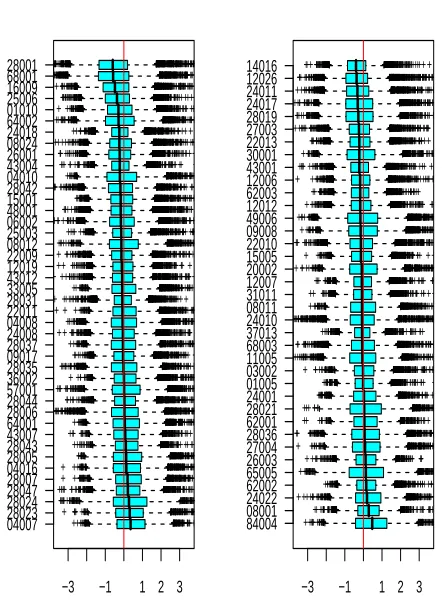
Fig. 1 summarizes all externally-Studentized residuals by
sample, arranged by phenotype. Even though there is no
single overwhelmingly outlying sample, several samples do
catch the eye. For example, residuals from samples
28001
and
68001
(
NEG
phenotype, top left) are predominantly
negative, and also exhibit relatively high variability. Residuals
from sample
84004
display high variability combined with a
positive tendency (
BCR/ABL
phenotype, bottom right). If a
sample’s expression levels are systematically higher or lower
+ +++++ +++ + +++++ ++ ++ ++++ +++++++ ++ ++++++++++++++ + + +++++++++ + ++++++ ++++++++++++ +++++++ +++ ++++ ++ +++ ++++++++++++ + +++++++++ + +++++ ++++++++ +++ ++ +++++++++++++++ ++++++++ +++ ++++++++++ +++++ +++++++++++ ++ ++++ +++++++++++ ++ + ++ +++++ +++ + +++ ++ ++++++++++++++++++++ +++++++++ ++ ++ +++++++ +++++++++++++++++++++++++++++++++++++++++++++++ ++++++ ++++++++ ++++++ ++++ ++++ + ++ ++ ++++++ ++++++++++++ ++++ +++ +++++++++ +++++++++ +++++++++++++++++ +++++ ++ +++++ +++++ +++ +++ ++++++++++++++++++++++++++++++++ + ++++ ++++ ++ ++++ ++ + +++ ++ + ++++++++++ ++++++++ ++++++ ++++ +++ +++++++ +++ +++++++++++ ++++++++++++ ++++++++++++ +++++ +++ +++++++++++++++ ++++++++++++++++++++++++++++++++++ ++++ ++++ +++ +++ ++++ +++++++ ++ ++ +++++++++ ++++++++++ +++ ++++ ++ +++++++++++++++ +++++ ++++++ ++ +++ ++++++++++++ ++++++++ ++++++ ++ +++++++ +++++++++++++++++++ ++ ++++++++++++ + ++++++++++++++++ +++++ +++ +++ +++++++++ + +++++ ++++++++++ ++ +++ +++++ +++ +++++++ ++++++ ++ ++ + ++++ ++++ +++++++ ++ ++ ++++ ++++++++++ +++++++ ++++++ ++++++ ++ ++++++++++++++ + + + +++ + +++++++ ++++++++ + + ++ ++++++ +++++++++++++++++++++++++++ ++ ++++ +++ ++++ + ++ +++++++++ ++ +++++++++++++++ +++ ++++++ ++ +++++ +++++ +++++++++++++++ +++++++ ++++++++++ +++ +++++++++++++++++++++++++++++++++++++++++++ ++++ ++ +++++++ ++ +++++ ++++++++++++ ++++++++++++++ +++++ ++++++++++++++++++ +++ +++++++++++++++ ++ +++ +++++ ++++++++++++ ++ ++++++ +++++++++++++++ +++++ +++ +++ + +++++ ++++++ +++++++++++ +++ +++ +++++++++++++++++++++ + ++++ +++ + ++++ ++++++++++++++++++++++++ ++++++++ ++++++++++++ ++++++++++++ +++++++ ++ ++++++++++++ ++++++++++ ++ ++++++ +++++++++++++ +++++++++++ +++++++++++++++++++++++++++++++++++++++++++++++++++ ++++++ +++++++++++++++++++++++++++++++++++++++++++++++++ ++++ + ++++++++++++++++++ ++ ++++++++++ ++++++++ +++ +++++++++++++ +++++++++ +++++++++ +++ +++++ ++++++++++ +++ +++++++ ++++++ ++++++ +++++++++++ +++++++++++ +++++ +++ +++++ + ++++ ++ ++++++ ++++++ ++ ++ ++++++ +++++++ ++ ++++ +++++++++ +++++++ +++++ ++++ +++++++++++++++++++++++++++ ++++++++++++++++++++++++++++++++++++++++++++++++++ ++++ + ++ + +++++++++ ++++ +++++++++++++++ ++ +++ ++ ++++++++++ +++++++++++ +++++++++++++++++++++++++++++++++++++++++++++++++++++++++++++++++++++ + +++ ++ +++++++ ++++ +++ + ++++ ++++++++ + +++++ +++++ ++ +++ +++++ +++ ++++++++++++++ ++ +++++++ +++ +++++++++++ ++ ++++++ ++++++ +++++++ ++++++++++++++++++++ + ++ +++++++++++++ ++++++ +++++++ ++++++ +++ +++ ++++++ ++++++++++++ +++ ++++++ +++ +++++++ ++++++ ++++++++ ++ + +++++++ + ++++ ++++++++++ ++++++++ +++ +++++++ ++ ++ ++++++++++++++++++++++++++++++++++ + + + ++++ ++++ + +++ +++++ +++++++ + ++++ +++++++++++++++ ++++ ++++++++++ ++++++++++++ ++++++++++ ++++ ++ ++++++++++++++ ++++ ++++++++ +++++ ++++++++++++++++++++++ +++++++++++++++++++++++++++++++++++++++++++++++++++++++ ++++++ + ++ ++ +++ + ++++ +++++++++ ++++++++ +++++ + +++ ++++ ++ +++ +++++++ +++++++++++++++++ ++++ + +++++++++ ++++ ++++++++++++++++++++++++ +++++ +++++++++++++++++++++++++++ +++ ++++++++ +++++++++++++++ +++++++++ ++ ++++++++++++++++++++++++++++++ +++ +++++++++++++++++++++++++++++++++++++++++++++++++++++++ + ++ +++ + + ++ +++++++ + + +++ ++++++ +++++ +++++++ ++++ +++++ ++++ ++++++ ++++ +++++++++++++++ + +++ +++ ++++++++++++++++++++++++++++++++++++++++++++++++++ ++++++++++++++ + +++++ +++ ++++ + ++ ++++ +++++++++++ ++++++++++ +++++ + ++ +++ ++ +++++++++++ +++++ ++++ +++ + +++++++++++++++++++++++++++++++++++++++++++ ++++++ +++++++++++++++++++++++++++++ + +++++++++++++ +++ ++++++++ +++ ++++++++ ++ +++++++ +++++++++++++++++ ++++++++++++++++++ ++++ +++++++++ +++++++++++++++++++++++++++++++++++++++++++++++++++++++ ++++ ++ ++ +++++++++ +++ +++++ +++++ ++ ++++++++++++++ ++++ ++++++++ ++ +++++ ++++ ++++++ ++ ++ +++++++++ +++++++++ +++++ +++++ + ++ ++++++++++++++++++ ++ +++++++++++++++ ++ +++++++++ +++++ ++ +++ +++ +++ +++++++ +++++++++++++++++ + ++++ + ++++++++ + ++++ + + ++ ++++ +++++++++++++++++++++++++++++++++++++++++++++++++++++++ +++++ +++++++++++ ++ ++ +++ ++++++ ++++ +++++++++++++++++++++ ++++++ ++ ++ ++++++ ++++++++++++++++++++++ ++++ +++ +++++++++++++ +++++++++ +++++ ++++++++ ++ + ++++++ ++ ++++++++ ++ ++ ++ +++++ +++++ ++++ +++++ +++ ++++++++++++++++++++ ++ ++++ + +++++++++++++++++++++++++++++++++++++++ ++++ + +++++ + ++++ ++++++++++ ++++++++++++++++++++ +++ ++++++++++++++++++++++++++++++++++++++++++++++++++++++++++++++++++++++++++++ ++++++++++ ++++++ +++++++++++++++++ +++ ++++ ++++++ +++++++++++++++++++++ ++ ++ ++++++++++++++ ++++++ +++ +++++++++++ +++++ ++++++++ ++ ++++++++ +++++ ++ ++ ++++++++++ +++ ++ ++ +++++++++++ ++++++++++ +++++++++ +++ ++++++++ ++++++ ++++++++++++++++ +++ +++ ++++++ ++ +++++++++++++++++++++ ++++++ +++++ ++ ++++++++++ ++++ ++++++++++++++++++++++++++++++ + +++++ + + +++ ++++++++++++++++ +++++++++ ++++ +++++++++++++++ +++++++++++++++++++ +++++++++++++++ ++ +++++++++++++++++++++++++++ +++++++++++++ + ++++ +++++++++++ +++ +++++++++ ++++++++++++ ++++++++ +++++++++++++ ++ +++++ ++ +++++++++++++++++++++++++++++++++++++++++++++++++++++++++++++++++++++++++++ ++++++++ ++++++++ +++++++++++++ ++ +++++++++++++++ +++++++++++ ++++++++++++++++++++++++++++ +++++++ ++++++++++++++++ +++++++++ ++++++++ +++++++++++++++++ ++ +++++++++++ + +++ ++++++ +++ ++++++++++++++ +++++++ +++++++++++++++++++++++++++++++++++++++++++++ ++++++++++ + + + +++++++ +++++ ++++++++ ++ ++++++ +++++++++++ +++++++++++++++ +++ ++ + +++++++++++++++++ +++++++++++++++++++++++++++++++++ +++++++++++++++++++++++++++++++++++++++++++++++++++++ ++++ ++++++++ +++++ ++++++++++ ++++++ +++ +++++++++ +++++ ++ ++++ + +++ ++ ++++++++++ +++ +++++ +++ +++ ++ +++++++++++++++++++++ +++++++ + +++++++++++ + ++++++++++ ++++++++++ +++ ++ + ++++ +++++++ +++++++++++++ ++++++ ++++++++++++++++ ++++++++ ++ ++++ +++++++++++++++++++++ ++++++++++++++++++ ++++++++++++++++++++++++++++++++++++++++++++++++++++++++++++ ++ +++ +++++ ++ ++ +++ ++++++ ++ ++ + +++++++++++++++++ ++++++++ +++++++ +++++++++ ++++++ ++++++++++++ +++ ++ +++++ +++++++++++++++ ++++ +++++++ ++ +++ +++++++++++++ +++++++++++++++++++++++++++++++++++ +++ + ++++ ++++ +++ +++ ++ ++ + +++++ +++ ++++++++++ +++ ++++++ ++ + ++++++++++++++++++++++++++++++++++++++++++++++++++++ +++ ++ ++ + +++ +++ + +++++ ++ + ++ ++++++++ +++ +++++++ +++++++++ + ++ + + +++++++++ +++ +++ +++ ++++ ++++++ +++++++++++++++++ ++++++ ++++++++++++++++++++++++ +++++ +++++++++++++++++++++++++++++++++++++++++++++++++++++++++++++++++++++++++++++++++++++++ ++++++++++ ++++ ++ +++ ++++++++++++ ++ +++ +++++ +++ +++++++++ +++ ++ +++++++ ++ +++++++++ +++ ++++++++ +++ +++ ++++++++++++ ++++++ ++++ + +++++++++ +++ +++++ +++++++++++++++ +++++ ++++++++++++++ +++ +++++++++++++ +++++++ ++++++ ++++ ++ +++ +++++++++++++++ +++ ++++++ + +++ ++ ++++++++ ++++++++ ++++++++++++++ +++++ ++++++++++++++++++++++++++++++++++++ +++ ++ +++++++++++++++ +++++ +++ ++++++++ ++++++++++ +++ ++++++++++++++++++++++++++++++++++++++++++++++++ + ++ + + + + + +++ + + ++ ++++++ + + + ++ ++ +++++++++++++++++++ +++ +++ +++++ ++++++++ +++++++ +++++++++ ++++++++++ +++++ +++++++ + + ++++++ ++ + + +++ +++ + +++ ++ +++ + + + + + +++ ++++++++++++++++++ ++++ +++++++++++ +++ ++++++++ +++ ++ ++ +++++++++++ +++ + ++++++ +++++++++++++++++++++++++++++ +++++ + ++ +++ +++++++ + ++ +++++++ +++++ +++ + +++++ ++ +++ ++ ++++++++++++++++++++++++++++++++++++++++++++++++++++++++ ++++ ++++++ +++++++++ ++ +++ +++++ +++ +++++++++++++++ +++ ++++++++ ++ +++++++++++ +++++++++++++++++++++++++++++++ ++++++++++++++++++++++++++++++++++ +++++++++++++++++++ +++ +++ + +++ +++++ ++ ++++ +++++ ++++++ ++++++ ++++++ ++ +++++++++++++ ++++++ +++++++++++ + +++ ++++++++++++ +++++++++++++++++++++++ +++++++++++++++++++ ++ ++ +++ + + ++ ++++++++++++++ +++++++++++++ ++++++ ++++ +++++++++ ++++ +++++ + + + ++++++++++++++++++ +++++ +++++++++++++++++++++++++++ +++++ +++++++++++++ +++++++++++++++ ++++++ + ++++++ ++ +++ + +++++++ + +++++++++ ++++++++++++++++++++++++ +++++++++++++++++++++++++++++++++++++++++++++++++++++++++++++ ++++++++++++++++++++++ +++ ++++++ + +++++ ++ ++++++ +++ +++++++++ + +++++++++++++ +++ +++ +++ ++++++++++++++ +++ +++ ++++++++++ +++++++++ ++++++ +++++++ + ++++++++++++++++++++ +++++++++ +++++++++ +++++++++ +++++++++++++++++++++++++++++++ +++ + ++ ++++++++ ++++++ + +++++ ++++++++ +++ ++ +++ ++ ++++++++ ++++++ +++ ++ + ++++ +++++++++++++++++ +++ +++ ++++++++++++++++++++++++++++++++ +++ +++ +++ ++ ++++++ ++ ++++++++ ++++++++++++++++++++++++++++++ +++++++++++++++++++++ + + +++++ +++++++++++++++++ +++++++++++++++++++ ++++++++++++++++++++++++++++++++++++++++++++++++++++++++++++++++++++++++++++++ +++++++ ++ ++ ++++++++ +++ ++++++++++++ +++ +++++++++++++ ++ ++ +++ ++++ +++ ++++++++++++++ ++ +++++ ++ ++ +++++++++ +++++++ ++ ++++++ ++ +++++ ++++ +++ ++++ ++++++++++++ +++++++++++++++++++++ ++ ++++++++++++ +++++++++++++++++ ++++ ++++++ ++ +++++++ ++++++++++ +++++++++++++ ++++++++++++++++++++++ +++++++++++++++++++++++++++++++++++ ++++++++++++++++ + +++ +++++ ++++++++++++ +++++++ ++++ +++++++ +++++++ +++++ + +++ ++++++++++++++++++ + +++ +++++++++++ +++ ++++++++ ++++++++++++ ++ ++ ++++++++++++ +++++++ + +++++++ ++++++ ++ ++++++ ++++ ++++++ +++++++++++++++++++++++++++++++++++++++++++++++++++++++++++++ + +++++ +++ ++++ +++++++++ ++ ++++++ + +++ ++ ++++++ +++++ ++ ++++ +++++ ++++ ++++++++++++++++++++ ++++++++ +++ +++ +++++++ ++ +++++++++ ++++++ ++ ++++ ++ ++++++ +++++ +++++++++ +++ ++ +++ ++++ +++ ++++++++++++++++++++++++++++++++ ++++++++++++++++++++ +++ +++++++++ ++++ ++++ + ++++ + ++ ++ ++ ++ + ++++++++ +++++ ++++ + + + ++++ +++++ + +++ ++++++++ ++ +++ ++ ++ + ++++++++++++++ ++++ ++++++ +++ +++ +++++++++++ + ++++ ++++ + ++++++++ ++++++++++++++++++++++++++++++++++++++++++++++++++++ +++ ++ +++ +++++++ ++++++++++++++++++++++++++ +++ +++++++++++++ ++++++ ++++ +++ ++ ++++++++++++++++++ +++ +++++++++++++++++++++++++++++++++++++++++++++++++ + + + ++ +++ ++ + ++++ +++++++++++++++++++++++++++ ++++ +++ +++ +++ ++++++++++ ++++ +++++++++++ +++++++++ +++++ +++++++++++++++++++++++ ++ ++++++++++++++++++++ ++++++++++++ ++++ ++++++++ + ++++++++ ++++++++++++ ++++++++++++++++ ++++++++ +++++++++ + +++ ++ ++ +++++ ++ ++ +++++++++ +++ +++++++++++++++++++++++++++++++++++++++++++++++++++++++++++++++++++++++++ +++++++++ ++ +++ ++++++++++ ++++ ++++ ++++ ++++++++++ + +++ +++ +++ ++++++ +++++++ ++++++ +++ ++++ ++ +++ +++++++ ++++++++++ ++ +++ +++++++++ +++++++++++ ++ +++++ +++++++ ++++++ ++ +++++++++++++ +++++ +++ ++++++ +++ +++++ ++++++++++ +++++++++++++++++++++++++ +++++++ +++++++++++++++++++++++++ ++++++ ++++++++++++++++++++++++++++++++ +++ ++ ++++++ ++ +++ +++ + +++ ++ ++++++ +++ +++++ +++++++++ ++++ +++ +++++ +++++ ++++++++++++ ++++++++++ +++++++ ++++++++
04007
28023
28024
28047
28007
04016
28005
28043
43007
64001
28006
28044
57001
36002
28035
09017
28037
24008
04008
22011
28031
33005
43012
12019
22009
08012
25003
06002
48001
15001
28042
04010
43004
26001
08024
24018
64002
01010
25006
16009
68001
28001
−3
−1
1 2 3
All NEG Residuals by Sample ( 4495 Genes )++ + ++ ++ + + ++++ + ++ ++ ++++++ ++++ +++ +++++++++++++++ ++++++ +++ ++++++++++ ++++++++++ + + +++ + +++++ +++++ +++++++++++++++++++++++++++++ ++ + +++++++++ ++++++ +++++++++++++++++++++++ +++ ++++++++++++++++ ++++ +++++++ ++ +++++++++++ +++++ +++++++ ++ ++ ++++++++++++++ +++ +++++ +++ ++++ ++++++++ +++ ++++++ ++ ++ +++++++++++++++++++++++ ++++ +++ +++++++++ + + ++++ ++++++++ + +++++++++++++++++ +++ +++++ +++++++++++++++++++++++++++++++++++ + + + +++++++ +++ ++++++ ++++++ ++++++++ +++ +++++++++ +++++++ ++++++ + ++ ++++++++++++++++ ++++ ++++++++++ +++++++++++ + +++++++++ ++++ +++++ +++ +++ ++++++++++++++++++++++ + + + ++++++++ +++++++++ + ++++++++++ + +++ +++++++ ++++ +++++++++ + + ++++++++ +++ ++ ++ +++ +++ ++++++ +++++++++++++++ +++++++++++++++ ++ ++++++++++++ +++ +++ ++++++++++ + + +++ +++++++ + + + + +++++ +++++ +++++ + ++++++++ ++ + ++ ++++++ +++++ +++++++ ++ ++++ +++ +++++ ++ +++++++ ++++++++++++++++++++ ++++++++++++++++++++++ ++++++++++++ +++ ++++++++++++++ ++++ +++++++ +++++++ ++++++ ++++ + +++ ++++ +++ + +++++ ++++ ++++ +++++++++ +++++++++++ ++++++++++++++++++++++++++++++++ + + + +++++ + + + + +++ + + ++ +++++++++ +++ ++++++++++ +++++++ ++++++ ++ +++++++++++++ +++ +++++ + ++++ + + +++++ +++++ + + +++ ++++++ + ++ +++++ ++++++++++++++++++ +++++ +++++++++++++ +++ ++ +++++++++++++ +++++++++ +++++++ +++++ +++ +++++++ ++ ++++ +++++ +++ ++++++++ + + + + ++ +++ + ++++ ++++ ++ ++++++ + +++++++++++++++++++++ +++++++++++ ++ ++ ++++++ ++++++ ++ +++ ++++++ ++ +++++ +++++ +++ ++++++++++++++ +++ + ++ ++++++ ++++++ +++ ++ ++++++ + ++++++++++ ++++++++++ ++++++++++ +++++++++++++++++++++++ +++ ++ +++ ++++++++++++++++ + +++++ ++ ++++++++ +++ ++++ ++++++++ + ++ ++ ++++++ +++++ +++++++++ + +++++++ +++ + ++++++ ++++++++++++++++++++++++ + ++++++++ ++++++++++ +++ +++++ +++++ ++++ + +++ +++++++ ++++ ++++++ +++++++++++ +++++ +++++++++++++++++++ +++ +++++++++++++++++++++++++++++++++++++++++ +++++ ++++++++++ ++ ++++ +++ ++++ ++ +++ +++++ +++++ ++ ++++ +++++++++++++++++ + ++++ +++++++++++++++ +++++++++++++++++++++++ ++++ ++ +++++++++++++++++++++++++ + ++ + +++ +++++ + ++ +++ ++++++ +++ +++ ++ +++++++++ ++++ +++++++++++++++ +++ ++++++++++++++ ++++++++ ++ + +++++++++++++++++++++ ++ +++++ ++++++++ ++ ++++++++++++ ++++ + +++ ++ +++++++ +++ + ++ ++++++++++++ +++++ ++ ++++++++ ++++++++++++++++++++++++++ +++++++++ ++++++++++ ++ +++++ +++ +++++++++ +++++++++++ ++ ++++++ + +++++++++++ ++++ ++++++ ++ ++++ ++++++++++ +++++ + +++ + ++ + ++ ++ +++ ++ + ++++ +++ +++++++++++ +++++++++++++++ +++++ + ++ + ++ +++++ + ++ +++ ++++++++++++ +++ ++++++ +++++++++++++ +++++++++++ ++++++++++ + + +++ ++ +++ + + + +++++++ +++++++ +++ + +++++++++ +++ ++ +++++ ++ ++ ++++ ++++++++++++++++++++++++++++++++++++++++++++++++ +++++++++++++++++++++++++++++++++++++ ++++++++++++++++++++++++++++++++++++++++++++++++++++++++++++ ++++++++++++++++++ ++++++++++ +++++++++ ++++++++++++ + +++ +++++++++++++++ +++++++++++++ +++++++++++++++++++++++++ ++++++ ++ +++++++++ ++++++ + ++++++++++++++ ++++++ +++++++++++ +++++++++++ ++++++++++++++++++++++++++++++++ ++++++++++++++++ +++ ++++++++ ++++++++++++++++++++++++++++++++++++++++++ ++ + + + + ++ + +++++++++++++ +++++++ ++++ +++++ ++ + ++ ++ +++++++++++++ ++++++ ++++++++ +++++++++++++++ ++++++++++++++++++++++++++++++++++++++++ + +++ + +++++++++++ +++++ + ++++ ++++++ ++++++++++++ +++++ +++++ ++ +++++++++++++ +++++++++++++++++++ ++++ +++++ +++++ ++++ ++++++++++ ++++++ ++ +++ ++++++ ++++ +++++++++ +++++++++++++++++++++++++++++++++++++++++++ ++++++++ ++++++ +++ ++ +++ +++++++++++++++++++++++++++++ ++++ ++++++++ +++++++++ +++ +++++++ +++++++++++ +++++ +++++++++ +++++++ + ++ +++ ++++++ ++++ +++++ +++++++++++++ +++++ ++++ ++ +++ ++++++++++++++++++++++++++++++++++++++++ + + + ++ ++ +++++++++++++++++++++++++++++++++ + +++++ ++++++++++++++ +++ ++++++++++++ +++ +++++++++++++++ ++++++++ +++++ +++++++ +++ +++++ +++ ++ ++++++++ ++ ++++++ +++ +++ ++ +++++++++++ ++++++++ +++++++++++++++++++++++++++++++++++++++++++++++++++++++++++++ + ++++++++++++++++++ ++ +++++++++++ ++++ ++++ ++++ +++++++ + ++ ++ +++++++++++++++++++++ ++++++++ ++ ++++++++++++++ +++++ +++++++ ++++++++ ++++++++++++ ++ ++++++++++++++++++++++++++++ ++ ++++++++++ +++ +++++++++++++ +++++++++++ ++++++++++++++++++ +++++++++++++++++++ + + + ++ +++++++ + ++ + ++ ++++++ ++++++++++ ++++++++++++ +++++++++++++++++ ++++ ++++++++ ++++++ +++++++++++++++++++++++++++++++++++++++++++++ ++++ ++ +++ +++++++ + ++ ++ ++ ++++++ ++++++++ ++++++++ +++++++ ++++++ +++ ++++ ++ ++++ ++ +++++++ +++ +++++++ ++++++ +++++ ++ +++++++ ++++ +++++++++ ++++ +++ +++ +++++++++++++ ++++ +++++++++++++++++++++ ++ + +++++ ++ ++++ ++ +++ +++++++ ++ ++++ +++++++++++ +++ +++ + +++++++++++ +++ ++ +++++ +++ ++ ++ +++++++++++++ ++++++++++++++++ ++++++++ ++ ++++++++++++++++++++++++++++ + + ++ ++ + + + ++ ++ ++++++++ +++ + +++++++ +++ + ++++ +++++++ +++++++ +++++++ +++++++++++++++++++++++++++++++++++++++++++++++++++++++++++++++++++++++++ + ++++++++ ++ +++++ +++ ++ +++++ ++++++++++++++ +++++++++++++++++++++++++++++++++++++++++++++++ ++ ++ ++++++++ +++++ ++++++++++++++++++++++++++++++++++++ + +++++ +++ ++++++++++++++++++ + + + +++ ++++++ + + +++++++ ++++ ++++ + + + ++ +++++ + + +++ + ++ ++ +++++ ++ ++++++++ +++ +++ + + +++ +++++++++++++ ++++ +++ +++ ++++++++++++++++++++++ +++++++++++++ ++ ++ ++++++++++ + +++ ++++++ ++ +++ ++++++++++++ ++++ ++ + +++++ + + ++ + +++++++++ + +++++++ ++ +++ +++++ +++ +++++ +++++ ++++ ++++++ ++++ +++++ +++++++ ++ ++ +++ +++++++++++++++++++++++++++ + +++++++++++++ + +++++++++++++++++ ++ ++ +++++++++++++ ++++++ +++++++ +++++ + ++++++++ +++++++++++ ++++++++++++++++++++ +++ ++++++++++ ++ ++++++ + +++++ +++ ++++++++++ ++++ +++ +++ ++++++++++ +++++++++++++ ++++++++++++++++++++++++++++++++++++++++++++++++++ ++ ++++ +++ ++ +++++++++ ++++ ++ +++ +++ ++ ++++++++ +++++++++++++ ++ ++++++++ ++++++++++++ + ++++++++++++++++++++ ++++++++++++++++++ + +++++++++++++++++++++ +++++++++++++++++++++++++++++++ + ++++ ++++++ +++++ ++++++++++++++++++++++++++++++++++++++++++++++++++++++ + +++ +++++ +++++++++++ ++++ ++ ++ ++ ++ +++++ ++ +++++++++++++ ++++++ ++ ++++ ++++++ ++ +++++++++++++++ +++++++++++++++++++++++ +++++++ +++++ ++++++ ++++++++++++ ++ + +++ + + ++ + ++ + ++++++++++++ +++++++ +++++++++++++++++++ +++ +++++ +++++++++++ + ++++++ ++++++++++++ +++++++++ + + +++++++++++++++++++ +++ +++++++++++++++++ ++++++++ + + ++ +++++++ ++++++++++++++++ ++ +++++++++++ ++ +++ ++++++++ +++++++++++++ +++++ ++++++++++ +++++++ ++ +++ ++++ ++++++ ++++++++++++++++++++++++++++++++++++++++++++++++++++++++++++++++++++++++++++++++++++++++++++++++++ ++++++++++++ ++++ +++++ +++ ++++++++++ ++++++ +++ ++++++++++++++++ + +++++++++ ++++++++++++++++++ ++++++++ +++++++++++++++++++++++ ++++++++++ ++++ ++++++++++++++ +++++++ + +++++++++++++++++ ++++++++ +++++++++++++++++++++++++++++++++++++++++++++ +++++++++++ ++ + ++ + ++ +++++++++ +++ + ++++ +++ +++++++++++++++ ++ +++ + ++++ + ++++ + ++ + + ++++ ++ ++ +++ ++++++ +++++++++++ +++ ++ +++++++++ + + +++ + ++++++++ ++++ ++++ ++++ +++ ++++++++++++ +++++++++++++++++++++++++++++++++++++++++++++++++++++++++++++++++ +++ +++++ +++ ++++ ++++ ++ + ++++ +++ ++++ + +++ +++ ++ +++ + ++++ ++ ++++ +++++ ++ + ++++++++++++++++++++++ +++++++++++ +++ ++ ++ +++++++++++++ ++++++++++++++++++++++++++++ +++++++++++++++ ++++ +++++++++++++++++++ ++ ++++++ +++++++++++++ +++++ +++++ +++++++++++++++++++++++++++ ++++++ + ++++ ++ + + +++++++++ ++++++++++++++ +++ + + + ++++++++ + +++++++ ++++ ++ + +++ ++++ + +++ ++ +++++++ ++++ +++++++ +++++++++++ ++++ ++++ ++++ +++++ +++++++++++++++++ +++++++++++++++++++++++++++++++++++++++++++++ +++++++++++++++ ++++++++++++++ ++++++++++ +++++++ ++++++++ +++ +++ +++++ +++++++++++ ++++++++++ +++++++++++ ++++++++++++++++++++++++++++ +++++++++++++++++++++++++++++++++++++++++++++++ +++ +++++++++++++++++++++++++++++++++++++++++++++++++++ +++++++ +++++++ +++++++++++ +++++++++++ +++++++ +++++++++++++++ +++++++++ ++++++ ++++++++++++++++++++++ + + + + ++ ++ +++ + ++ + + ++ ++ ++++ ++ +++++++ + + +++++ ++++++++++++ ++++++++++ +++ ++++ +++++++++++++++++++++++++++++++++++ +++++++++++++++++++++++++++++++++++++++++++++++++++++++++++++++++++++++++ ++ + ++++ +++ +++ +++ ++++ +++++ +++++++ ++++++ ++++++++ ++ +++++ ++ ++++++ +++ +++ +++++++ ++ ++++++ ++++++++ ++++++++ ++++++++ +++++++ +++++++++++++++++ ++ ++ ++++++ ++++++++ ++++ +++++++++ ++++ +++ ++ ++++ ++ ++ +++++++ +++++++++ + +++++++++ +++ +++ +++++++++++++++++++++++ ++++++ ++++++++ +++++++ ++++++++++ ++++++++ ++++++ ++++++++++ +++++++++++++++++++++++++++ ++++ ++++++++++++++ +++++++++++++++ +++ + + ++ + + ++ ++++++++++++++++++ ++++++ ++++ + +++++ +++++++++ ++++++++++++++ ++++++++++ +++++ +++++++++++++++++++++++++++++++ +++ + ++++++++++++ +++ +++ +++ +++++ ++++ ++++ ++ ++++ ++++++ ++ ++++ +++++ ++++++++++++++ ++++++ ++ +++++++++++++++++++++++++++ +++++ ++++++++++++++++ ++++++ +++++++++++++++++++++ ++++++++++++++++++++++++++++++++++++++++++++++++++++++++++++++ + ++++++++ ++++++ ++ ++++ +++++ + ++ +++++ +++++ ++++++++++++ ++++++++ ++++++ ++ ++++ ++++++++++ ++++++++++++++++++ + ++ +++++++++++ ++++++++++++ +++++ ++++++++++ ++ ++++ +++ + ++++ ++++++++++ ++++++ ++++++ +++++++++++ +++++ + ++++ ++++++++++++++++++++++++++++ + +++++++++++++++++++++++++++++++++++++
84004
08001
24022
62002
65005
26003
27004
28036
62001
28021
24001
01005
03002
11005
68003
37013
24010
08011
31011
12007
20002
15005
22010
09008
49006
12012
62003
12006
43001
30001
22013
27003
28019
24017
24011
12026
14016
−3
−1
1 2 3
All BCR/ABL Residuals by Sample ( 4495 Genes )Fig. 1. Raw externally-Studentized residuals from linear model of gene expression on phenotype for the ALL dataset, grouped by sample, arranged by phenotype (NEGon left,BCR/ABLon right) and sorted by each sample’s median residual.
across the board, it is impossible to tell whether this is due to
real biological differences or due to a normalization offset; we
suspect that the latter case is more common. It is interesting
to note that the dataset had already been normalized during
preprocessing with all 12625 features present. Apparently, the
4495 features shown on Fig. 1 are different enough from the
rest to somewhat disrupt the early normalization. Moreover,
removal of the average per-gene baseline via regression,
and Studentization of the residuals, seem to improve our
sensitivity to normalization offsets. In any case, whether
corrective normalization action is warranted – and also whether
a phenotype-only model fits the data well – becomes clearer
upon observing GS-level residuals.
3.1.2 GSEA Diagnostics
Figure 2 displays a heatmap
of GS residuals, with chromosome bands in rows and
samples in columns. Red indicates positive values and
blue negative values. In order to avoid overlaps, only the
Fig. 2. GS residuals from the linear model of gene expression on phenotype, for each lowest-level chromosome band (row) and sample (column). Residuals in each row were standardized to have mean zero and standard deviation1. Heatmap colors change in increments of0.8 (on the normalized scale), with reds positive and blues negative. The horizonal band at the top indicates the value of thekinetvariable: red for hyperdiploid, grey for diploid and white for unknown.
correlation, allowing us to detect patterns deviating from model
fit – whether they occur by sample or by gene-set.
One of the samples identified above as having low
residuals,
28001
, is visible as a narrow predominantly-blue
vertical strip (Fig. 2, somewhat right of center). This indicates
no association between chromosomal loci and low expression
levels for this sample; unless we realign expression levels on
the filtered dataset (most simply by removal of sample-specific
medians), sample
28001
– and quite possibly others with
smaller offsets – are likely to appear as outliers during more
detailed analysis. More interesting from a modeling perspective
is the apparent block or checkerboard pattern of the heatmap.
This pattern indicates a potential association between groups of
samples and overall expression levels at certain chromosomal
locations; an association not explained by the phenotype-only
model. In particular, there is a relatively tight cluster of
20
samples (left-hand side of map), whose expression pattern
is roughly the opposite of most other samples. Among the
dataset’s 21 descriptive variables, we identified the “
kinet
”
variable to be most strongly associated with the pattern-induced
grouping of samples (Chi-square p-value conditional on the
clustering:
<
0
.
001
). This variable indicates whether the
sample is classified as hyperdiploid. The association between
hyperdiploidy and gene expression of chromosomal loci or
complete chromosomes among pediatric ALL patients, has
been well-documented in research (Ross
et al.
, 2003; Teixeira
and Heim, 2005), and we can plausibly assume it holds for
adult patients as well. The
kinet
variable is illustrated as
a colored band at the top of Fig. 2, with red indicating
hyperdiploid samples, grey diploid samples, and white samples
of unknown status. Even though only
19
of
79
samples are
hyperdiploid, they form a clear majority in the
20
-sample
cluster described above, and are further differentiated from
diploid samples within that cluster as well. We concluded that
it may be useful to add
kinet
to the model.
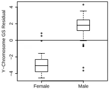
Another variable that is known with certainty to be
associated with chromosome-level expression differences
is sex. Females do not have the Y chromosome, and
therefore observed expression differences for non-autosomal
Y chromosome genes can serve several functions at once: a
test of microarray technology, a test of GSEA methodology
and a test for data-entry errors. Since the Y chromosome has
relatively few genes, it is represented in Fig. 2 by two rows
only, making its effect hard to detect at this level. A direct
inspection of GS residuals, with the gene-set defined as the
11 non-autosomal Y chromosome genes in our filtered dataset,
reveals the expected strong sex-related pattern – albeit with
some noise (Fig. 3). In fact, several samples’ GS residuals
deviate from their sex baseline so strongly towards the other
sex, as to suggest a possible sex mis-assignment in the dataset
annotation. A more careful analysis led us to conclude beyond
reasonable doubt, that two females have been misassigned as
males. Additionally, up to three males have apparently been
misassigned in the opposite direction, though the evidence is
somewhat weaker.
2For subsequent analysis in this article, we
have reassigned two samples to female and one sample to male.
An additional sample with a missing sex entry was identified as
male by its Y chromosome expression patterns.
Female Male
−4
−2
0
2
4
Y−Chromosome GS Residual
Fig. 3. Boxplot of GS residuals, calculated on the set of non-autosomal genes on the Y-chromosome, obtained from a linear model with only phenotype as predictor and grouped by sex.
−0.6
−0.4
−0.2
0.0
0.2
0.4
0.6
0.8
Log Expression Relative to Baseline
1 2 3 4 5 6 7 8 9 10111213141516171819202122 X Y +
+ +
+ +
+
+ + +
+ +
+
+ +
+ + +
+ +
+ +
+
+ +
B
B B
B B
B
B B
B B B
B
B B
B B
B
B B
B B
B
B B
H
H
H
H H
H
H H
H H
H
H
H H
H H
H
H H
H H
H
H H
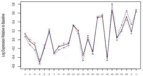
Fig. 4. Complete-chromosome mean expression levels relative to the median gene, as found by the 3-covariate model. Shown are the
baseline mean (NEG-diploid, black and ’+’ signs), the BCR/ABL
-diploid mean (red, dots and ’B’) and theNEG-hyperdiploid mean (blue, dashes and ’H’). All estimates are for male samples; the female-sample pattern was nearly identical, except for the Y chromosome.
3.2 GSEA Using the Expanded Model
3.2.1 Chromosome-Level Patterns
The GSEA procedure
was repeated with the changes indicated above – adding sex
and hyperdiploidy to the model, relabeling the sex entries
of three samples, and re-centering each sample’s expression
values by its median to diminish the impact of outlying
samples. Four samples with missing data for hyperdiploidy
were dropped from the analysis, leaving us with
n
= 75
.
It is of interest to compare the evaluation of the phenotype
effect before and after model expansion. There are minor
changes: the correlation between phenotype-effect
t
-statistics
generated by the two models is 0.99. We performed
GS-level inference to see if the minor variations between the
two models are localized to certain gene-sets. Inference was
obtained via sample-label permutation as explained above.
For the expanded model, care must be taken to permute
sample labels only within groups that have the same sex and
hyperdiploidy status. The test was performed only for the
leaves
of the chromosomal-loci tree, using
5000
permutations.
Overall, the 3-covariate model’s inference is somewhat more
conservative, and less tilted towards over-expressed bands.
However, there is substantial agreement between the significant
chromosomal-loci lists generated via the two models.
3At the other end of the chromosomal-loci hierarchy,
Fig. 4 shows complete-chromosome mean expression trends
calculated using the
3
-covariate model. Even for normal
samples (black line) there are marked inter-chromosome
differences, as is known from literature (Caron
et al.
,
2001).
BCR/ABL
’s trend (red dots) is almost indistinguishable
from the normal group, with the biggest gap observed at
chromosome 22, which is directly affected by that phenotype’s
anomaly. The hyperdiploid trend (blue dashes), though
3 see Supplement C for a significant loci list according to the 3
-covariate model.
following the normal group’s general trend, exhibits much
larger deviations from it – with chromosomes 19, 21, 22
and X most strongly over-expressed and chromosomes 3
and 13 most strongly under-expressed. All these effects
are statistically significant at the
0
.
05
false-discovery-rate
level (FDR, Benjamini and Hochberg, 1995; Benjamini and
Yekutieli, 2001). The sex covariate (trend not shown) has
negligible effect, except for the Y chromosome.
These hyperdiploidy-related differences raise the question
whether they are the result of individual hyperdiploid samples
exhibiting aneuploidy while others have normal expression
levels, or of a subtle expression shift across the entire
hyperdiploid group. In the former case, chromosome-level
GS residuals of samples with abnormal DNA copy number
should be flagged as gross outliers. Figure 5 displays a map
of these outliers, using GS residuals from an intercept-only
model. Outliers were identified via standard robust location and
scale methods (Huber, 1981), using a numerically generated
outlier-free reference distribution (Wisnowski
et al.
, 2001),
and FDR thresholds of
0
.
05
,
0
.
1
and
0
.
2
. We imposed the
additional constraint that the sample’s average expression for
the chromosome in question must differ from the median of
all samples by a relative amount of at least
1 : 6
(similarly
to Hertzberg
et al.
(2007)’s approach which was tested against
verified aneuploidies).
4Most hyperdiploid samples, and about
a dozen diploid samples, are flagged for at least one aneuploidy.
Observing Fig. 5 from the perspective of chromosomes,
chromosome X is by far the most prevalent, with 12 samples
flagged as potential multisomies at the
0
.
2
FDR level. The
next most prevalent multisomies are of chromosomes 21 and
14, respectively. Equally interesting are some chromosomes
absent from Fig. 5, because they have no flagged samples.
These include chromosomes 19 and 22, identified in Fig. 4 as
over-expressed by the hyperdiploid group, and chromosomes 3
and 13, identified as under-expressed. Sample-level inspection
reveals that these chromosomes are mildly over- or
under-expressed across the board, i.e., the second of the two potential
explanations suggested above seems to hold for them.
3.2.2 Influence Analysis
Beside identifying outliers,
res-earchers may need to answer the practical question: how
strongly does a specific outlying sample affect model
estimates? This is where Cook’s
D
, mentioned above, can be
useful. For the phenotype-only model, which splits the dataset
into two roughly equal-sized groups of
42
and
37
, no sample
is influential enough to cause concern – not even
28001
. The
story is somewhat different under the
3
-covariate model, where
both the female and hyperdiploid groups are much smaller.
Fig. 6 summarizes all
∆
kivalues for lowest-level chromosome
bands, by sample. Two samples belonging to hyperdiploid
female subjects (far right) have much larger overall influence
than most other samples. However, even they are not dominant
01010 08024 24001 24010 28006 28031 28036 28044 43001 64001 84004 04008 09008 15005 24017 28005 28019 28021 28024 28035 30001 36002 43007 48001 62001 64002 X 21 20 18 17 14 12 11 10 9 8 7 5 4 2
Fig. 5. Map of suspected aneuploidies in the ALL dataset, by chromosome (rows) and sample (columns). Red-brown hues correspond to extra copies, and blue hues to missing copies. Dark,
medium and light shades correspond to FDR levels of0.05,0.1and
0.2, respectively. The top bar indicates hyperdiploidy, as in Fig. 2. Samples and chromosomes with no flags have been omitted.
+ + + + + + + + + + + + + + ++ + + + ++ +++ + + + + + ++ + + + + + ++ + + +++ + + + + + + + + + + ++ + + + + + + ++ + + + + + + + + + + ++ + + + ++ + + + + + ++ ++ + + +++ + + + + + ++ + + + ++ + + + + + + + + + + ++ + + + + + + + + + + + + + + + + + + + + ++ + + + + + + + + + + + + + ++ + + + + + + + + + + + + ++ + + + + + + + + + + + + + + + + + + + + + + + ++ + ++ + ++ + + + + + + + + + + + ++ + + + + + + + + + + + + + + + + + + + + + +++ + + + ++ + + + + ++ + + + + + + + + ++ + + + + ++ + + + + + + + ++ + + + + + + + + + + + ++ + + + + + + + + ++ + + + ++ + ++ + + + + + + + + + + + + + + + + + + + + + + + + + + + + + + + + + + + + + + + + +++ + + + + + ++ ++ + + + + + ++ + + + ++ + + + ++ + + + + + + + + + + + + ++ + ++ + ++ + + + + + + + + + + + + + + + + + + ++ + + + + ++ + + + + + + + + + + + + + + + + + ++ ++ ++ + + + ++ + 0.00 0.05 0.10 0.15 0.20 0.25 0.30 0.35
Fig. 6. Chromosome-band root-mean Cook’sDvalues, summarized by sample, for the 3-covariate model. Samples are ordered by mean.
to the point of questioning the validity of hyperdiploidy or sex
effect inference.
4 DISCUSSION
Diagnostics,
an indispensable and versatile component
of regression analysis, are especially useful for finding
unexpected data patterns. On the single dataset used here for
demonstration, diagnostics have helped us recognize the need
to realign expression values; decide whether the sex covariate
has been entered in error for certain samples; explore model
expansion; and pinpoint suspected individual aneuploidies.
5Some of the uses of diagnostics can be formalized and
even automated (see Supplements B and D); others, such as
recognizing that there may be a Y-chromosome problem or
interpreting Fig. 2, are more exploratory and intuition-driven.
Software tools used to produce the analysis reported here
are publicly available as Bioconductor package
GSEAlm
.
6Researchers wishing to perform the main regression analysis
using a package of their choice, can still take advantage of
GSEAlm
’s diagnostic features by extracting residuals using
lmPerGene
followed by
getResidPerGene
. Detailed
information appears in the package’s vignette and manual
pages. The ALL dataset is available as Bioconductor package
ALL
.
FUNDING
This work was supported by the United States National
Institutes of Health [grant numbers NHGRI-1-P41-HG004059,
P50-CA-083636 (Ovarian SPORE)].
ACKNOWLEDGEMENTS
The authors thank S. Chiaretti and J. Ritz for making the
ALL dataset available, and C. Lottaz for a summarized and
preprocessed version of the St. Jude dataset used in Supplement
D. We also thank the anonymous referees for a timely review
that helped improve this manuscript.
REFERENCES
Benjamini, Y. and Hochberg, Y. (1995). Controlling the false discovery rate - a practical and powerful approach to multiple testing.J Roy. Stat. Soc. B,57(1), 289–300.
Benjamini, Y. and Yekutieli, D. (2001). The control of the false discovery rate in multiple testing under dependency.Ann. Stat.,29(4), 1165–1188. Caron, H.et al.(2001). The human transcriptome map: Clustering of highly
expressed genes in chromosomal domains.Science,291(5507), 1289–1292. Chiaretti, S.et al. (2004). Gene expression profile of adult T-cell acute
lymphocytic leukemia identifies distinct subsets of patients with different response to therapy and survival.Blood,103, 2771–2778.
5 Regarding aneuploidies, following a referee’s suggestion we applied
our residuals method to the St. Jude pediatric ALL dataset (Rosset al., 2003), on which Hertzberget al.(2007)’s expression-based aneuploidy detection method was optimized. For that dataset, cytogenetic information on chromosome 21 is available. Our method, lifted “as is” from the ALL dataset and applied to the St. Jude dataset with no further optimization, exhibits somewhat weaker sensitivity but somewhat better specificity than Hertzberget al.(2007). More details can be found in Supplement D.
6 Included in this package is a function to test a single covariate’s
Cook, R. and Weisberg, S. (1982). Residuals and Influence in Regression. Monographs on Statistics and Applied Probability. Chapman and Hall. Efron, B. (2007). Correlation and large-scale simultaneous significance testing.
J. Am. Stat. Assoc.,102, 93–103.
Ernst, M. (2004). Permutation methods: A basis for exact inference. Stat. Sci.,
19(4), 686–696.
Goeman, J.et al.(2004). A global test for groups of genes: testing association with a clinical outcome.Bioinformatics,20(1), 93–99.
Hertzberg, L.et al.(2007). Prediction of chromosomal aneuploidy from gene expression data.Genes Chromosome Cancer,46(1), 75–86.
Huber, P. J. (1981).Robust statistics. John Wiley & Sons Inc., New York. Wiley Series in Probability and Mathematical Statistics.
Hummel, M.et al.(2008). GlobalANCOVA: exploration and assessment of gene group effects.Bioinformatics,24(1), 78–85.
Jiang, Z. and Gentleman, R. (2007). Extensions to gene set enrichment analysis.
Bioinformatics,23, 306–313.
Kim, S.-Y. and Volsky, D. (2005). Page: Parametric analysis of gene set enrichment.BMC Bioinformatics,6;144.
Kong, S.et al.(2006). A multivariate approach for integrating genome-wide expression data and biological knowledge. Bioinformatics,22(19), 2373– 2380.
Mootha, V. K.et al.(2003). PGC-1α-responsive genes involved in oxidative phosphorylation are coordinately downregulated in human diabetes. Nat.
Genet.,34, 267–273.
Neter, J.et al.(1996). Applied Linear Statistical Models. McGraw-Hill Companies, Inc.
Nilsson, B.et al.(2008). An improved method for detecting and delineating genomic regions with altered gene expression in cancer.Genome Biol.,9(1), R13.
Pollack, J.et al.(2002). Microarray analysis reveals a major direct role of DNA copy number alteration in the transcriptional program of human breast tumors.
Proc. Nat. Acad. Sci.,99(20), 12963–12968.
Ross, M.et al.(2003). Classification of pediatric acute lymphoblastic leukemia by gene expression profiling.Blood,102, 2951–2959.
Subramanian, A.et al.(2005). Gene set enrichment analysis: A knowledge-based approach for interpreting genome-wide expression profiles.Proc. Nat. Acad. Sci.,102(43), 15545–15550.
Teixeira, M. and Heim, S. (2005). Multiple numerical chromosome aberrations in cancer: what are their causes and what are their consequences?Sem. Canc. Biol.,15(1), 3–12.
Tian, L.et al.(2005). Discovering statistically significant pathways in expression profiling studies.Proc. Nat. Acad. Sci.,102(38), 13544–13549.