Survey on Different Method to Improve Performance of The Round Robin Scheduling Algorithm Bhavin Fataniya 1, Manoj Patel2

(1)

© 2018 IJSRSET | Volume 4 | Issue 2 | Print ISSN: 2395-1990 | Online ISSN : 2394-4099 National Conference on Advanced Research Trends in Information and Computing Technologies (NCARTICT-2018), Department of IT, L. D. College of Engineering,

Ahmedabad, Gujarat, India. In association with International Journal of Scientific Research in Science, Engineering and Technology

IJSRSET184213 | Accepted : 15 Jan 2018 | Published 22 Jan 2018 | January-February-2018 [ (4)2 : 69-77 ]

₆₉

Survey on Different Method to Improve Performance of The

Round Robin Scheduling Algorithm

Bhavin Fataniya

1

, Manoj Patel

2

1_{M.E(I.T) Student, I.T Department, L.D College Of Engineering, Ahmedabad, Gujarat, India} 2_{Assistant Prof., I.T Department, L.D College Of Engineering, Ahmedabad, Gujarat, India}

ABSTRACT

Round Robin (RR) scheduling algorithm is the widely used scheduling algorithm in multitasking and real time environment. Its performance highly depends on a Time Quantum, which is a predefined amount of time assigned by CPU to every task to be executed. If we chose the less time quantum then context switch is high and if we chose the high time quantum then its leads to First-Come-First-Serve (FCFS). So, the performance of the system totally depends upon the choice of optimal time quantum. In this paper I will survey a different method to improve performance of the round robin scheduling algorithm using dynamic time quantum and also compare different method to each other to see the performance of the algorithm with respect to turn around time, waiting time, number of context switch.

Keywords: Round Robin,Dynamic Time Quantum.

I.

INTRODUCTION

CPU scheduling is one of the fundamental features that an Operating System (OS) needs to perform multitasking. CPU scheduling means allocation of sufficient resources to a process being executed. The policy of CPU scheduling is to maximize the efficiency of the CPU. This efficiency includes maximizing the throughput, minimizing context switches, Average Waiting Time (AWT) and Average Turnaround Time (ATT) of the processes in ready queue. Throughput can be defined as the number of processes executed per unit cycle. The process waiting time of a process is the time it spends in ready queue before its execution.Turn around time is the sum of waiting and the execution time of a process.CPU scheduling algorithms are subdivided in to two main categories. A non-preemptive algorithm is the one in which CPU is allocated to a process till completion of its execution while in a preemptive algorithm, a higher priority process can block currently running process. Or we may simply conclude that if there are n processes in a ready queue, a non-preemptive process can have only n − 1 context switches. While a

preemptive process can have more context switches. Some of the algorithms that have been developed and implemented are as follows;

First Come First Serve (FCFS) [9]: As obvious from the name,FCFS processes the jobs in the order in which they arrive in the ready queue.

Shortest Job First (SJF) [9]: In this algorithm, the ready queue is first sorted on ascending order of burst times of the processes arrived in it. Then the processes are assigned CPU in sequence.This algorithm is optimal than others in most cases. But in SJF,we must be able to have a pre-knowledge of burst times of all the processes which is difficult practically. Moreover, it can cause starvation for longer processes.

(2)

International Journal of Scientific Research in Science, Engineering and Technology (ijsrset.com)

₇₀

focusing on efficiency constraints of CPU. So, it may

cause best and worst cases depending on burst times of corresponding processes. FCFS and SJF, both are non-preemptive algorithms. But PS can be of both typei.e. preemptive or non-preemptive. If the currently executing process can continue its execution on arrival of a higher priority process, then it is a non-preemptive priority scheduling .On the other hand, if the process is blocked on arrival of a higher priority process, it is a preemptive priority scheduling.

Round Robin (RR) [9]: This algorithm allocates CPU to all processes for an equal time interval. A process is blocked and put at the end of ready queue after a constant time slice, known as Time Quantum. This process is assigned CPU time again once the execution of all other processes in their respective time quanta. The efficiency of Round Robin depends entirely on the time quantum selected. If the time quantum is selected too large, the algorithm will become FCFS. While on the other hand, if the quantum is much small, it will yield much overhead and larger average waiting and turnaround times .With advancement in technology, many Round Robin algorithms based on dynamic time quantum have been developed. In this, a dynamic time quantum is chosen instead of a constant time quantum. It may be changed after a cycle or just after an arrival of next process in ready queue .In next section we will see the original round robin algorithms, some of the problem of round robin algorithms and survey of different method to improve performance of the round robin scheduling algorithm using dynamic time quantum and also compare different method to each other to see the performance of the algorithm with respect to turn around time, waiting time ,number of context switch.

II.

ROUND ROBIN ALGORITHM

It is one of the oldest, simplest, fairest and most widely used scheduling algorithms, designed especially for time-sharing systems. A small unit of time, called time slice or quantum is defined. All run able processes are kept in a circular queue. The CPU scheduler goes around this queue, allocating the CPU to each process for a time interval of quantum. New processes are added to the tail of the queue. The CPU scheduler picks the first process from the queue, sets a timer to interrupt after time quantum, and dispatches the process. If the process is still running at the end of the quantum, the CPU is

pre-empted and the process is added to the tail of the queue. If the process finishes before the end of the quantum, the process itself releases the CPU voluntarily. In either case, the CPU scheduler assigns the CPU to the next process in the ready queue. Every time a process is granted the CPU, a context switch occurs, which adds overhead to the process execution time.

An example of round robin algorithm is given below:

Process AT BT

P1 0 40

P2 0 55

P3 0 60

P4 0 90

P5 0 102 Time quantum=25.

Figure 1. Gantt chart for round robin

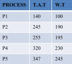
Turn-around time and waiting time for above example is calculated in below table.

PROCESS T.A.T W.T

P1 140 100

P2 245 190

P3 255 195

P4 320 230

P5 347 245

III. ROUND ROBIN PROBLEM

(3)

₇₁

quantum.Increase in quantum time - cause less

context-switch,lesser turn-around time but can cause high response time, and waiting time. Decrease in quantum time-cause less waiting time and response time but can cause high turn-around time and high no of context-switch Hence a medium sized time quantum can reduce all the factors to some extent. medium sized time quantum can be achieved by using dynamic time quantum method. now we will see different method based on dynamic time quantum.

IV. LITERATURE REVIEW OF DIFFERENT ROUND

ROBIN ALGORITHM BASED ON DYNAMIC TIME

QUANTUM.

Assumptions

AT=arrival time, BT=burst time, T.A.T=turn-around time, W.T=waiting time, CS= context switch, C.T=completion time.

During analysis we have considered CPU bound processes only. In each test case 5 independent processes are analyzed in uni-processor environment. Corresponding burst time and arrival time of processes are known before execution. all the arrival time and burst time is in M.S(milli second).Arrival time and burst time of different case is below.

Case 1. arrival time is same [8]

Process AT BT

P1 0 105

P2 0 60

P3 0 120

P4 0 48

P5 0 75

Case 2. arrival time is different [8]

Process AT BT

P1 0 45

P2 5 90

P3 8 70

P4 15 38

P5 20 55

In our analysis for various algorithm we have used above two table(case 1,case 2) to see the performance of particular algorithms.Turn-around time and waiting time can be calculated using below formula.

T.A.T=C.T-A.T. W.T=TA.T-B.T.

A. Modified Round Robin Algorithm for Resource Allocation based on average.[3]

a) Methodology

Pandaba Pradhan,Prafulla Ku. Behera, B N B Ray [3] proposes an algorithm MRRA to improve the performance of Round Robin. In MRRA for each cycle the average of burst time of the processes is calculated and used as time quantum.

Step-1:process arrive in ready queue based on A.T.

Step-2:sort the process based on B.T of process found on ready queue.

Step-3:find time quantum using average of B.T of process which is placed on ready queue.

Step-4:now assign this time quantum to all process which is loaded in ready queue.

Step-5:if process B.T-time quantum=0 then terminate that process.

Step-6:IF process B.T-TIME QUANTUM!=0 then put that process at end of ready queue. Continue with step:2 to step:6 until all process are completed.

Step-6:calculate T.A.T,W.T,NO OF C.S.

Case 1. arrival time is same

The Gantt chart shown as in Figure 2

Figure 2. Gantt chart for MRRA [3] for same arrival time of process.

(4)

₇₂

P1 369 264

P2 108 48

P3 408 288

P4 48 0

P5 183 108

Case 2. arrival time is different

Figure 3. Gantt chart for MRRA [3] for different arrival time of process.

Turn-around time and waiting time for above example is calculated in below table

P1 45 0

P2 293 203

P3 263 193

P4 68 30

P5 118 63

B. Self-Adjustment Time Quantum in Round Robin Algorithm Depending on Burst Time of the Now Running Processes (SRBRR ALGO).[2]

b) Methodology

Rami J. Matarneh [2] proposes an algorithm SRBRR to improve the performance of Round Robin. In SRBRR for each cycle the median of burst time of the processes is calculated and used as time quantum.In other word time quantum is calculated using TQ=median(BT of process in ready queue).Median is calculated using below formula.

where, Y is the number located in the middle of a group of numbers arranged in ascending order.

Consider below example

Step-1:process arrive in ready queue based on A.T. Step-2:find time quantum using median of B.T of process which is placed on ready queue.

Step-5:IF process B.T-TIME QUANTUM!=0 then put that process at end of ready queue. Continue with step:2 to step:6 until all process completed.

The Gantt chart shown as in Figure 4.

Figure 4. Gantt chart for SRBRR [2] for same arrival time of process.

P1 105 0

P2 165 105

P3 285 165

P4 333 285

P5 408 333

Case 2. arrival time is different.

Figure 5. Gantt chart for SRBRR [2] for different arrival time of process

(5)

₇₃

P2 293 203

P3 269 199

P4 176 138

P5 258 203

C.Implementation of Alternating Median Based Round Robin Scheduling Algorithm[5]

c)

Methodology

The proposed algorithm uses a set of two time quanta for scheduling the ready queue. These time quanta are used alternately in cycles of scheduling. Before the first cycle of scheduling starts, one of the time quanta is set equal to the median of burst time of processes present in the ready queue while the other one is calculated as the difference between the highest value of burst times and the median of burst times of processes present in the ready queue.The two-time quanta remain fixed throughout scheduling and are not recalculated until the architecture of the ready queue gets changed by the arrival of a new process.The larger time quantum is used if even number of cycles of scheduling are completed while the smaller time quantum is used if the odd number of cycles of scheduling are completed. Therefore, the two-time quanta are used alternately in cycles of scheduling.

Step-1:process arrive in ready queue based on A.T. Step-2:sort the process based on B.T of process found on ready queue.

Step-3:now calculate time quantum 1=median of B.T of process which is present in ready queue and time quantum 2=high B.T- time quantum 1.

Step-4:now assign this time quantum 1 if even number of cycle is completed and assign time quantum 2 if odd number of cycle completed to all process which is loaded in ready queue.

Step-6:IF process B.T-TIME QUANTUM!=0 then put that process at end of ready queue.Continue with step:2 to step:7 until all process completed.

Figure 6. Gantt chart for AMBRR [5] for same arrival time of process

PROCESS T.A.T W.T

P1 366 261

P2 108 48

P3 408 288

P4 48 0

P5 183 108

D. Design of A Modulus Based Round Robin Scheduling Algorithm(MB ALGO)[4]

d)

Methodology

The Modulus Based (MB) algorithm has been devised on the basis of two scheduling algorithms namely MRR(AVG) algorithm and SRBRR(median) algorithm. This algorithm gives the results intermediate between both of its parent algorithms. if we encounter scenarios where the MRR(Avg) algorithm behaves more efficiently than the SRBRR algorithm or vice versa, then we can select the given MB algorithm in order to get more stable results.

The formula of calculation of

time quantum Q is given in equation.

Step-3: using above formula find time quantum of B.T of process which is placed on ready queue.

(6)

₇₄

Step-6:IF process B.T-TIME QUANTUM!=0 then put

that process at end of ready queue.Continue with step:2 to step:5 until all process completed.

Figure 7:Gantt chart for MB algorithm[4] for same arrival time of process

P1 366 261

P2 108 48

P3 408 288

P4 48 0

P5 183 108

Case 2. arrival time is different.

Figure 8. Gantt chart for MB [4] for different arrival time of process

P1 45 0

P2 293 203

P3 262 192

P4 68 30

P5 118 63

E. An Improved Dynamic Round Robin Scheduling Algorithm Based on a Variant Quantum Time(DRR ALGORITHM)[1]

e)

Methodology

Step-3: if the arrival time of all process is same then first time quantum is calculated using below formula

T.Q1=Σ two high B.T/2.

Then second time quantum is calculated using below formula.

T.Q2=Σ of high remaining B.T and T.Q1 /2.

Step-4:now assign this time quantum 1(T.Q1) to first cycle and for remaining cycle used T.Q2.

Step-8 : if the arrival time of all process is different than time quantum is calculated using below formula. T.Q1=B.T OF FIRST ARRIVED PROCESS

T.Q2= (Σ of high remaining B.T and T.Q1 /2) – (Σ OF THE TWO LOOWEST REMAINING AT/2) (used only once time)

T.Q3== (Σ of high remaining B.T and T.Q1 /2) – (LOOWEST REMAINING AT/2)

Step-9:now assign this time quantum 1(T.Q1) to first cycle and for second cycle used T.Q2 and for remaining cycle used T.Q3.

(7)

₇₅

Turn-around time and waiting time for above example is

calculated in below table.

P1 288 183

P2 108 48

P3 408 288

P4 48 0

P5 183 108

Case 2. arrival time is different

Figure 10. Gantt chart for DRR ALGORITHM [1] for different arrival time of process

P1 45 0

P2 293 203

P3 261 191

P4 68 30

P5 118 63

F. Improved Round Robin Scheduling using Dynamic Time Quantum.(IRR ALGORITHM)[6]

f)

Methodology

Debashree Nayak [6] proposes an algorithm IRR to improve the performance of Round Robin. In IRR,for each cycle the median of burst time of the processes is calculated.Median is calculated using below formula.

where, Y is the number located in the middle of a group of numbers arranged in ascending order. Then time quantum is calculated using below formula T.Q= ( MEDIAN + HIGH B.T ) / 2

Step-1:process arrive in ready queue based on A.T.

Step-2:sort the process which found in ready queue.

Step-3:using above formula find time quantum of B.T of process which is placed on ready queue.

Figure 11. Gantt chart for IRR ALGORITHM [6] for same arrival time of process.

P1 385 280

P2 108 48

P3 408 288

P4 48 0

P5 183 108

(8)

₇₆

Figure 12. Gantt chart for IRR ALGORITHM [6] for

different arrival time of process.

P1 45 0

P2 293 203

P3 200 130

P4 68 30

P5 118 63

V.

COMPARISON

Section IV describe the all dynamic quantum based round robin algorithm All the above described algorithms except SRBRR[2], first sort processes on ascending order of their burst times.This tends their algorithm towards SJF and most of algorithms take advantage of optimization of SJF rather than their own algorithms. Moreover,the sorting on ascending order is itself problam.It is important to note that the time quantum calculated by the MRR(Avg)[3] algorithm which varies greatly due to possibility of smaller or larger differences in execution times of tasks.Hence this average may be larger than median of burst times of all the tasks giving smaller T.A.T and less number of context switches but larger response time and W.T.Hence SRBRR algorithm is more stable than the MRR(AVG) algorithm if sorting of process is used in SRBRR[10].but in original SRBRR sorting of process is not used so its leads to F.C.F.S in case of process arrival time is same.SRBRR is perfectly work if arrival time of process is different. The calculation of the time quantum of MB[4] algorithm is a computationally intensive task that consumes a bulk of time for the calculation of Median and the Average of burst times of tasks in each cycle..In this section we will see the Comparison of each algorithm based on average turn-around

time(A.T.A.T),average waiting time(A.W.T) and No of C.S.

Figure 14. A.T.A.T and A.W.T of when all process arrived at same time(case:1)

Figure 15. number of context switch when all process arrived at same time.(case:1).

Above Figure 14 and 15 show the comparison between A.T.A.T ,A.W.T and NO of C.S for all algorithms which was describe in section IV.From above graph we will conclude that D.R.R algorithm give the best result compare to all other algorithms. It will give best average turn-around time and best average waiting time.No of C.S is less in SARR algorithm but its leads to FCFS so this is not useful. D.R.R[1] algorithm give less number of context switch compare to remaining algorithm.

(9)

₇₇

Figure 16. A.T.A.T and A.W.T when all process arrived

at different time(case:2)

Figure 17. number of context switch when all process arrived at different time.(case:2)

VI. CONCLUSION

Different scheduling algorithms are reviewed in this paper.section IV describe the overall working of all dynamic quantum based round robin algorithm.section V describe the comparison of all algorithm. At last we conclude that D.R.R[1] algorithm is more stable than all other algorithm in case of arrival time of all process is same and I.R.R[6] algorithm is more accurate than all other algorithm in case of different arrival time of process.

VII. REFERENCES

[1]. A. Alsheikhy, R. Ammar, and R. Elfouly, "An improved dynamic Round Robin scheduling algorithm based on a variant quantum time",IEEE, 2015 11th International Computer Engineering Conference (ICENCO), 2015, pp. 98-104.

[2]. Rami J. Matarneh,"Self-Adjustment Time Quantum in Round Robin Algorithm Depending

on Burst Time of Now Running Processes", American J. of Applied Sciences 6(10): 1831 -1837,2009.

[3]. Pandaba Pradhan, Prafulla Ku. Behera and B N B Ray, "Modified Round Robin Algorithm for Resource Allocation in Cloud Computing ", ScienceDirect, Procedia Computer Science 85 ( 2016 ) 878 – 890,2016.

[4]. Salman Arif, Saad Rehman and Farhan Riaz "Design of A Modulus Based Round Robin Scheduling Algorithm",IEEE, 9th Malaysian Software Engineering Conference, Dec. 2015 [5]. Salman Arif,Naveed Ghaffar,Ali Javed

"Implementation of Alternating Median Based Round Robin Scheduling Algorithm",IEEE, International Conference on Computer and Information Technology,2016.

[6]. Debashree Nayak, Sanjeev Kumar Malla and Debashree Debadarshini "Improved Round Robin Scheduling using Dynamic Time Quantum", International Journal of Computer Applications (0975 – 8887) Volume 38– No.5, January 2012 [7]. A. Noon,A. Kalakech and S. Kadry,"A New

Round Robin Based Scheduling Algorithm for Operating Systems: Dynamic Quantum Using the Mean Average", International Journal of Computer Science Issues (T.TSI),Vol.3,Issue 3,No. 1,pp. 224-229,May 2011.

[8]. Amar Ranjan Dash, Sandipta kumar Sahu and Sanjay Kumar Samantra"AN OPTIMIZED ROUND ROBIN CPU SCHEDULING ALGORITHM WITH DYNAMIC TIME QUANTUM" International Journal of Computer Science, Engineering and Information Technology (IJCSEIT), Vol. 5,No.1, February 2015.

[9]. Sonia Zauaoui,lotfi Boussaid and Abdellatif Mtibaa, "CPU scheduling algorithms case and comparative study",17th international conference on sciences and techniques of automatic control &

computer engineering=STA

2016,sousse,Tunisia,Decmber,2016.

[10]. H.S.Behera, R. Mohanty and Debashree Nayak "A New Proposed Dynamic Quantum with Re-Adjusted Round Robin Scheduling Algorithm and Its Performance.

Survey on Different Method to Improve Performance of The Round Robin Scheduling Algorithm Bhavin Fataniya 1, Manoj Patel2

69

Survey on Different Method to Improve Performance of The

Round Robin Scheduling Algorithm

Bhavin Fataniya

, Manoj Patel

ABSTRACT

I.

70

II.

III.

ROUND ROBIN PROBLEM

71

IV.

LITERATURE REVIEW OF DIFFERENT ROUND

72

73

c)

Methodology

d)

Methodology

The formula of calculation of

time quantum Q is given in equation.

74

e)

Methodology

75

f)

Methodology

76

V.

77

VI.

CONCLUSION

VII.

REFERENCES

₆₉

₇₀

₇₁

₇₂

₇₃

₇₄

₇₅

₇₆

₇₇