Visual Programming of MPI Applications:
Debugging, Performance Analysis, and Performance
Prediction
Stanislav B¨ohm, Marek Bˇeh´alek, Ondˇrej Meca, and Martin ˇSurkovsk´y
V ˇSB Technical University of Ostrava 17. listopadu 15/2172, 708 33 Ostrava
{stanislav.bohm, marek.behalek, ondrej.meca, martin.surkovsky}@vsb.cz
Abstract. In our research, we try to simplify the development of parallel appli-cations in the area of the scientific and engineering computations for distributed memory systems. The difficulties of this task lie not only in programming itself, but also in a complexity of supportive activities like debugging and performance analy-ses. We are developing a unifying framework where it is possible to create parallel applications and perform various supportive activities. The unifying element, that interconnects all these activities, is our visual model that is inspired by Colored Petri Nets. It is used to define the parallel behavior and the same model is used to show the inner state of the developed application back to the user. This paper presents how to extend this approach for debugging, tracing, and performance predictions. It also presents benefits obtained by their interconnection. The presented ideas are integrated into our open source tool Kaira (http://verif.cs.vsb.cz/kaira). Kaira is a prototyping tool, where a user can implement his/her ideas and experiment with them in a short time, create a real running program and verify its performance and scalability.
Keywords:MPI, debugging, performance analysis, performance prediction.
1.
Introduction
Clusters – parallel computers with distributed memory – represent one of the most wide spread category of computers for scientific and engineering computations. A lot of people can participate in developing software for them, but there are well-known difficulties of parallel programming. Therefore, for many non-experts in the area of parallel comput-ing, it may be difficult to make their programs run in parallel. The industrial standard for programming computational applications in the area of distributed memory systems isMessage Passing Interface(MPI)1. MPI specifies a library for C and Fortran for send-ing messages between processes. Even if it is relatively simple to use, it represents quite a low-level interface. There are tools likeUnified Parallel C2that simplify creating par-allel applications, but the complexity of their development lies also in other supportive activities like debugging, performance analyzing, verification, etc. Therefore, even an ex-perienced programmer of sequential applications can spend a lot of time learning a new set of complex tools.
1
http://www.mpi-forum.org/ 2
The overall goal of our research is to reduce complexity in parallel programming. We want to build a unifying prototyping framework for creating, debugging, analyzing, and formally verifying parallel applications, where a user can implement his/her ideas in a short time and experiment with them, create a real running program and verify its performance and scalability. The central role in our approach plays an abstract computa-tional model and visual programming (based on Coloured Petri Nets [10]) that we use for development of MPI applications [2–4].
This article extends paper [5], which presents the usage of our approach for debugging and performance analyses. By a performance analysis, we mean an analysis of a real run of an application. More precisely, we are focused on tracing, where the behavior of an application is recorded and such record is analyzed. In this paper, we moreover introduce another way of obtaining a performance characteristic of examined applications performance predictions – the behavior of the application is evaluated in a simulated environment. The presented ideas are implemented inKaira(http://verif.cs.vsb.cz/kaira); an open source tool that we are developing.
The contribution of this paper are the following: We show how can be an abstract com-putational model integrated into the environment used by practitioners (C++ and MPI) in a way that provides a unified approach to debugging, performance analysis and perfor-mance prediction. These activities are unified in the sense of control, configuration and results displaying.
In the following section, selected supportive tools from the area of parallel program-ming are briefly introduced. Sections 3 and 4 describes tool Kaira and implemented sup-portive activities. Section 5 provides a demonstration of the proposed approach. The last section concludes presented ideas.
2.
Related Works
This section briefly introduces tools for debugging, performance analyzing, and perfor-mance predicting in the area of MPI applications. For a more detailed comparison we refer to [2].
An MPI application runs on each computing node like a normal program; therefore, we can use standard tools likeGDB3 for debugging. This approach is sufficient to find some types of bugs, but the major disadvantage is completely separated instances of the supportive tool for each process. There are specialized debuggers to overcome this issue like: Distributed Debugging Tool4 or TotalView5. They provide the same functionality like ordinary debuggers (stack traces, breakpoints, memory watches), but they allow to debug a distributed application as a single piece. Besides these tools, there are also non-interactive tools likeMPI Parallel Environment6. It provides additional features over MPI, like displaying traces of MPI calls or real-time animations of communication. More about debugging in MPI environment (and related difficulties) can be found in [17, 18].
As with debugging, tools for non-distributed application may be used to analyze the performance of MPI applications. However it brings similar problems, because
measure-3
http://www.gnu.org/software/gdb/ 4http://www.allinea.com/products/ddt/ 5
http://www.roguewave.com/ 6
ments are performed separately for each MPI process. ToolsGprof7andCallgrind8can be named as examples of such tools. They usually provide a summary of events (profiles) of the application’s run in a form of call time sums and frequencies for each function. The approach of generating profiles can be extended into the environment of MPI. It is implemented byPgprof9ormpiP10.
However, the profile is not always as useful for parallel applications as it is for sequen-tial applications. The reason is that computational times are affected by various commu-nications costs, waiting times, synchronization, and so forth. Therefore many analytical tools for parallel programs record atraceof an application’s run where important events are stored with time stamps. The trace allows a more precise reconstruction and analysis of an application’s behavior.Scalasca[8, 7] andTAU[16] can be named as examples of tracing tools. The drawback of this approach is a greater overhead in comparison with gathering a profile. Moreover, a trace grows with the length of a program’s run and with the number of processes. Its size can be a major issue and post-processing huge tracelogs may be computationally demanding. For trace visualizations, there are specialized tools likeVampir[12] orParaver[14].
For performance predictions, two major approaches exist:analytical approachesand predictions bysimulations. An example of the analytic approach can be found in [11]. It consists of a handmade formal analysis of an algorithm. The result is given as a formula describing how the computational time depends on the characteristics of a given computer. The analytical approach is out of the scope of this paper and the more automatic approach based on predictions by simulations will be considered.
Tools offering simulations fall into two categories:online simulatorsandoffline sim-ulators. An online simulator directly executes the application and mimics the behavior of the target platform. It is implemented in toolsBigSim[21] andSimGrid[6]. Because of the direct execution, the major challenge is to reduce the demands on the CPU and memory. These tools allow skipping of some computations and can simulate delays that would be caused by executing these computations. It works only for applications with a data-independent behavior, because some parts are not really computed. Many practical applications satisfy this condition and this approach can provide good predictions in a relatively short time. Another important aspect is the complexity of the network simu-lation. The most precise method for the network simulation is a packet-level simulation (MPI-NetSim[13]) but it can be very resource consuming. The other way (used in most simulators) is a usage of a simple analytical model, for exampleBigNetSim(the network simulator for BigSim). Results of a simulation are often provided in the form of a trace; therefore, existing tools for displaying traces can be used.
Offline simulators ([19, 20, 9]) use a trace of an application’s run as the input instead of the application itself. The tracelog is replayed in conditions of the simulated platform to obtain predictions. The structure of communication is replayed as was recorded in the trace; computing and waiting times are modified according to the target platform. This way provides predictions while using fewer computations than online simulators, but the problems occur for applications where the structure of the communication is not fixed.
7
http://sourceware.org/binutils/docs/gprof/ 8http://valgrind.org/docs/manual/cl-manual.html 9
http://www.pgroup.com/products/pgprof.htm 10
In such cases, because of the different order of message arrivals, the program can get to different states and send different messages than recorded. The reader can find more detailed surveys about performance prediction tools in [1, 15].
3.
Tool Kaira
This section serves as an overview for our tool Kaira; for more details see [2–5]. Our goal is to simplify the development of distributed applications using MPI and create an environment where all supportive activities are unified under one concept.
The key aspect of our tool is the usage of a visual model. It was chosen to obtain an easy and clear way how to describe and expose parallel behavior of applications. The other reason was that a distributed state of the application can be shown through such model. The representation of an inner-state of distributed applications by a proper visual model can be more convenient than traditional ways like stack-traces of processes and memory watches. With this feature, we can provide visual simulations where a user can observe a behavior of developed applications. This can be used for incomplete applications from an early stage of the development. In a common way of developing MPI programs, it may often takes a long time to get the developed application into a state where its behavior can be observed. Moreover, we use the same visual model for mentioned activities and it is a natural unifying element as will be demonstrated later.
On the other hand, we donotwant to create applications completely through the visual programming. Sequential parts of the developed application are written in the standard programming language (C++) and combined with the visual model that catchesparallel aspectsandcommunication. We want to avoid huge unclear visual diagrams; therefore, we visually represent only what is considered as “hard” in parallel programming. Ordinary sequential codes are written in a textual language. Moreover, this design allows for an easy integration of existing C++ codes and libraries. C++ was chosen as one of major programming languages with a large variety of existing libraries.
It is important to mention that our tool isnotan automatic parallelization tool. Kaira does not discover parallelisms in applications. The user has to explicitly define them, however they are defined in a high-level way and the tool derives implementation details. Semantics of our visual language is based on Coloured Petri nets (CPNs)[10]. In gen-eral, Petri nets are formalism for the description of parallel processes. They also provide a well-established terminology, a natural visual representation for visual editing of models, and their simulations. Modeling toolCPN Tools11 was also the great inspiration for us; especially for the visualization of the model.
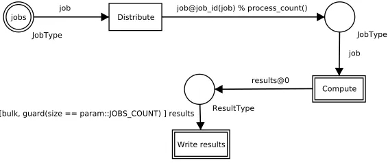
To demonstrate how our model works, let us consider the model in Figure 1. It presents a problem where some jobs are distributed across computing nodes and results are sent back to process 0. When all the results arrive, they are written into a file. Circles (places in terminology of Petri nets) represent memory spaces. Boxes (transitions) represent ac-tions. Arcs run from places to transition (input arcs) or from transition to places (output arcs). Places contain values (tokens). Input arcs specify which tokens a transition needs to beenabled. An enabled transition can be executed. When the transition is executed, it takes tokens from places according to input arcs. After finishing the computation of the
11
transition, new tokens are placed into places according to output arcs. In CPNs, places store tokens as multisets, in our approach we use queues. CPNs formalism was designed as a general modeling language and multisets are suitable for this purpose. But in compu-tational programs, it is usually desired to reduce nondeterminism of applications and for this purpose, queues are more convenient.
A double border of a transition means that there is a C++ function inside and it is executed whenever the transition is fired. A double border around of a place indicates an associated C++ function creating the place’s initial content (in this example, places are initialized only in process 0). Arcs’ inscriptions use C++ enriched by several simple constructions. A computation described by this model runs on every process. Arc expres-sions containing “@” define interprocess communication. The expression after “@” sign defines a target process where tokens will be transferred.
Fig. 1.A simple model in Kaira
3.1. Example: Heat flow with load balancing
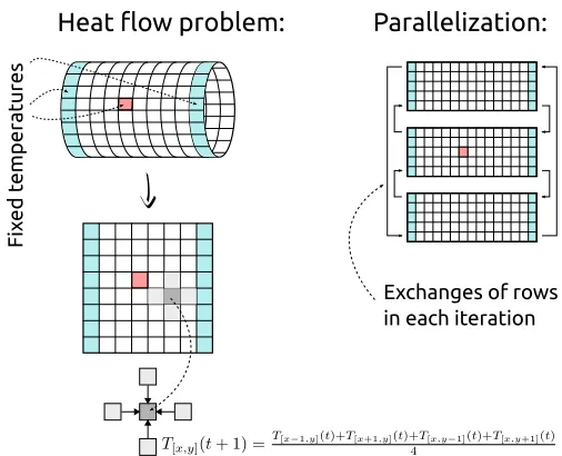
As a more advance example, we use the heat flow problem on the surface of a cylinder. The borders of its lateral area have a fixed temperature and one fixed point in the area is heated. The goal is to compute a heat distribution on the lateral area. In the presented solution, the surface is divided into discrete points that form a grid as it is depicted in Figure 2. Temperatures are computed by an iterative method; a new temperature of a point is computed as an average temperature of its surrounding four points.
This approach can be easily parallelized by splitting this grid into parts; each part is assigned to one process. In this example, we assume that the grid is split by horizontal cuts. No communication is needed to compute new temperatures of inner points of the assigned area. To compute temperatures in the top and bottom row, the process needs to know rows directly above and below this area. Therefore each process exchanges its border rows with neighbors in each iteration.
in cooperation with its neighbors. When an imbalance is detected then some rows are transferred to a faster neighbor.
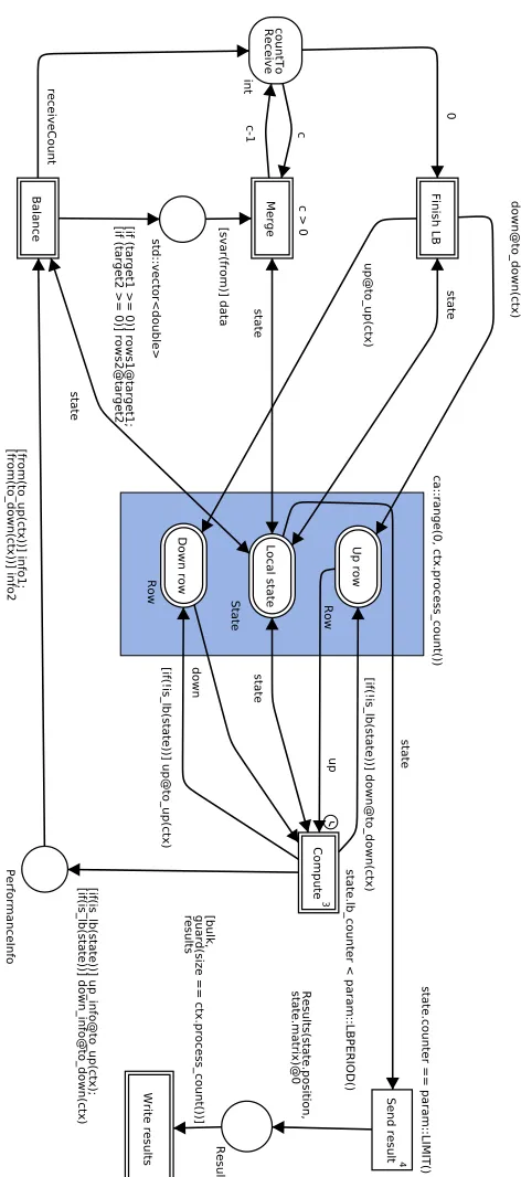
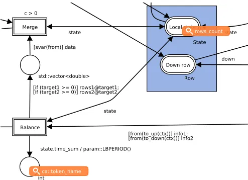
The implementation of this problem in Kaira is depicted in Figure 3 and Listing 1.1. TransitionComputeexecutes a single iteration of the algorithm. It takes a process’ part of the grid and two rows, one from the above neighbor and one from the below one. It updates the grid and sends top and bottom rows to its neighbors. When the desired number of iterations (parameterLIMIT) is reached then the results are sent to process 0 where they are written into a file.
ParameterLB_PERIODcontrols how often (in the number of iterations) balancing is performed. When balancing occurs,Computedoes not send border rows but sends its own performance information to its neighbors; it is the time spent in the computing phase and the number of rows in its own part of the grid. TransitionBalancedetermines how many rows are needed to exchange for balancing computational times. The formula is based on solving the equation: lm−∆s
m =
ln+∆
sn , where∆is the number of rows that should be
sent from the process to the neighbor process,lm(ln) is the number of own (neighbor’s)
rows, andsm (sn) is own (neighbor’s) performance – a number of rows computed per
second. If b∆c > 0 thenBalance sends rows to the neighbor. In each process, place countToReceiveindicates how many neighbors will send their rows to this process. This value is monitored because it is important not to resume the computation in a process until balancing with both neighbors is resolved; otherwise, the process would work with an invalid part of a grid and send wrong border rows. TransitionMerge adds received rows into the local part of the grid. Transition Finish LB finishes the balancing, it can be fired when all local balancing exchanges of rows are processed (i.e.countToReceive contains zero). The transition resets variablelb_counterand sends border rows to its neighbors; therefore the normal computation is resumed.
The init area (depicted as a blue rectangle) is used to set up initial values of places not only in process 0 but over specified processes (all processes in our case).
The clock symbol on the left side of transition Computemeans that the transition gains access to a clock. It is used for the computation current performance of the node, i.e. measure how much time it was spent on computations in transitionCompute.
4.
Features of Kaira
The main purpose of Kaira as a development environment is to create an application. In Kaira, visual models together with C++ sequential codes can be created and edited. From such model, the tools can automatically generate a stand-alone MPI application. Besides this primary purpose, Kaira provides additional features for application developed in our formalism. In this paper, we are focused on the situation when an application or its prototype is working and we want to analyze it. This section describes features related to debugging, performance analysis, and performance prediction.
4.1. Simulations
Listing 1.1.Head-code for the example of heat flow with load balancing
struct PerformanceInfo {
long time; /* Duration of computations in the last balancing period (ms) */
int rows; /* Number of rows processed in the last balancing period */ };
typedef std::vector<double> Row;
typedef std::vector<Row> Rows;
struct State {
State(int size_x, int size_y, int position) : matrix(size_x, size_y),
position(position),
counter(0), lb_counter(0), time_sum(0) {}
DoubleMatrix matrix;
int position; /* The position of the local grid part */
int counter; /* The counter of iterations */
int lb_counter; /* Number of iterations
from last load balancing */
int time_sum; /* Time spent in the computational phase
from last load balancing */ };
struct Results {
Results(int position, const DoubleMatrix &matrix) : position(position), matrix(matrix) {}
int position;
Parallelization:
Heat
fl
ow problem:
Exchanges of rows in each iteration
Fix
ed t
emperatures
Fig. 2.The heat flow problem on a cylinder and the used method of parallelization
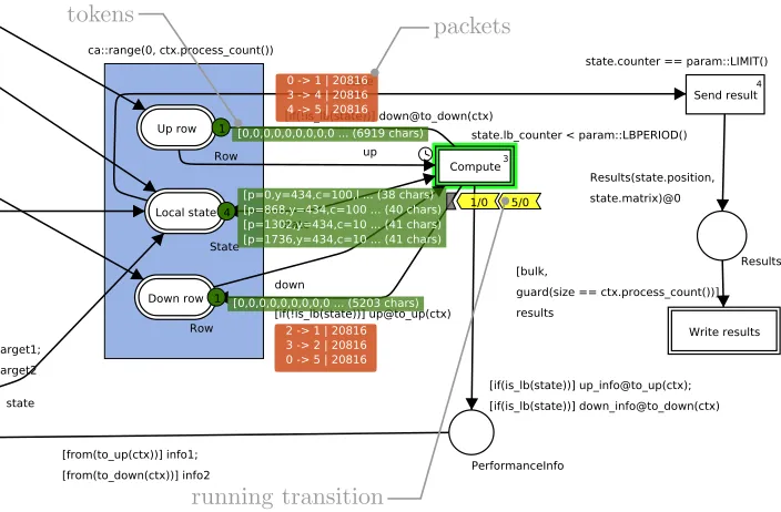
in the form of labels over the original model (see Figure 4). Two types of information are depicted:
– Tokens in places (The state of memory)
– Packets transported between nodes (The state of the communication environment)
These two types of information completely describe a distributed state of the applica-tion. The user can control the behavior of the application by the two basic actions:start an enabled transitionandreceive a message from a communication layer. By executing these two types of actions, the application can be brought to any reachable state. The model naturally hides irrelevant states during sequential computations and only aspects important to parallel execution are visible and controllable.
Kaira does not catch intermediate states during sequential computations of transitions. But still it allows putting the distributed application into any reachable state. The number of observable states is smaller than in a classic debugger and it allows to store all states showed during a simulation with a reasonable memory consumption, and the user may browse in the history of the execution.
Fig. 4.The model in the simulator. The full picture of the net is in Figure 3.
4.2. Tracing
An application developed in Kaira can be generated in the tracing mode. Such application records its own run into atracelog. When the application finishes its run, the tracelog can be loaded back into Kaira and used for thevisual replayor for a graphical representation of performance data. Generally, issues with such post-mortem analysis can be categorized into these basic groups:selection what to measure,instrumentationandpresentation of results.
Tracelogs can be useful both for performance analyses and debugging. In the case of debugging, we usually want to collect detailed information of the run for the reconstruc-tion of the cause of the problem. In the case of performance analyses, we want to discover performance issues and therefore need to measure a run with time characteristics as close as possible to real runs of the application. But the measurement itself creates an overhead that devalues the gathered information about performance. Therefore, it is important to specify what to store in the tracelog in both cases. In common tracers, specifications of measurements are usually implemented as a list of functions that we want to measure/fil-ter out. But it may be a non-trivial task to assemble such a list, especially in the case when we use some third-party libraries. It often needs some experience to recognize what can be safely thrown away.
and it is obvious what information will be gained or lost after switching on or off each setting. Moreover, our approach also allows for more detailed tracing. It is implemented as connecting arbitrary C++ functions to places. These functions determine what will be stored into the trace.
The second task is theinstrumentation, i.e. putting the measuring code inside into the application. In our case, Kaira can automatically place the measuring codes during the process of generation of a parallel application. Parallel and communication parts are gen-erated from the model, therefore we know where are interesting places to put measuring codes. By this approach, we can obtain a traced version of the application that does not depend on a compiler or a computer architecture. In contrast to a standard profiler or de-bugger for generic applications, we do not have to deal with a machine code or manual instrumentation.
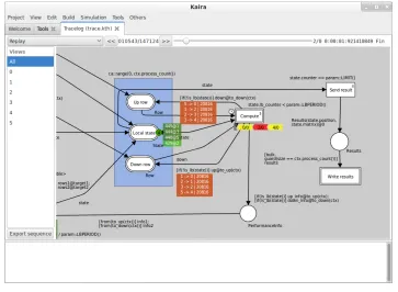
As we already said, the results are presented to the user in the form of a visual replay or as a graphical representation of performance data. In the replay, data stored in tracelogs are shown in the same way as in the simulator, thus as the original model with tokens in places, running transitions and packets in the communication layer (Figure 6). The user can jump to any state in the recorded run. Our tool also provides standard charts like a normal profiler, and additionally, information is presented using the terms of the model. For example, the utilization of processes (Figure 7), the numbers of tokens in places, etc.
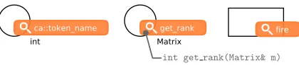
Fig. 5.Tracing labels, from left: Tracing names of tokens that arrive into the place; tracing values obtained by applying a function to each token arriving to this place; tracing transition firing.
4.3. Combination of tracing and debugging
Combination of tracing and debugging is implemented throughcontrol sequences. This feature naturally connects the infrastructure of our simulator with tracing abilities. A con-trol sequence is a list containing actions. Each action is one of two basic types from Section 4 (starting transitions and receiving packets). Actions contain information about the process where the activity is executed, the transition’s name (in the case of transition firing) and the source process of the message (in the case of receiving packets). When we store this information we are able to repeat the run of the application.
Fig. 6.The screenshot of a replay. The full picture of the net is in Figure 3.
Listing 1.2.A simple linear model of communication
ca::IntTime packet_time(casr::Context &ctx,
int source_id, int target_id, size_t size) {
const ca::IntTime latency = 5847; // [ns]
double bandwidth = 1.98059; // [byte/ns]
return latency + size / bandwidth; }
possible to add a whole new debugging transition. Now, it is possible to get the applica-tion again into the state before the problem by replaying the sequence in the simulator, but this time, we have the ability to obtain more information about the problem because of the modified version of the application.
4.4. Performance prediction
The performance prediction in Kaira is implemented as online simulations, i.e. a full computation of the program is performed in a simulated environment. The communication layer is simulated through an analytical model. In Kaira, there is not a fixed number of models, but the user may specify any model as a C++ function in a similar way as C++ sequential codes are edited in transitions or places. This function is called for each packet and returns a time needed to transfer the packet. The basic information like the size of the packet and process id of the sender and the receiver is passed to this function. A simple linear model is shown in Listing 1.2.
Additionally,casr::Contextenables the access to information about the value of the global clock and the current workload of the network between each pair of processes. Therefore more sophisticated models can be defined; models that reflect an overall situa-tion in the network or models with dynamic changes of the bandwidth in time.
The model of communication is not the only configurable setting. In Kaira, execution times of each transition and size of data transferred through each arc can be arbitrary modified. It is designed to answering questions like “what will be the overall effect when a code in a transition is optimized and is 20% faster than before the optimization”. However it can be also used for reducing a computation time. Predictions can be performed with smaller data while the behavior of the net is simulated with the original data size. The former is demonstrated in Section 5.
The configuration of this feature is specified in the same way as for tracing, i.e. as labels placed into the net (the example in Figure 8). In the case of a transition, the expres-sion in the label specifies how the running time is modified. The transition is computed as usual, but the program in the simulator behaves as if the computational time of the transi-tion is the time obtained from the expression in the label. In the expression, an instance of
casr::Contextis accessible through variablectxand variabletransitionTime
expressions on input arcs of the transition can be used in the label, hence the simulated computational times may depend on computed data.
The configuration for arcs works in a similar way by modifying the sizes of tokens produced by an arc. This value is used when a token is transferred through the network; the receiver obtains the data as they are sent, but the network simulation considers modified sizes of packets. Variable sizecan be used in the label and it enables access to the original size of the data.
Kaira additionally offers a special clock. It runs like an ordinary clock in a normal run, but it may be arbitrarily modified in a simulation in the same way as running times of transitions. A transition using this clock is depicted with a small clock symbol on the left side. The clock provides methodstic()andtoc()wheretoc()returns the time elapsed from the last call oftic(). In the simulated run, the user may provide an expression that is called after eachtoc()and modifies the returned time.
The simulated program produces a tracelog where the simulated run is recorded. It uses the same infrastructure as was described in the text above, including the way in which a measurement is specified and the results are post-processed. It provides richer possibilities for tracing than do many of existing prediction tools, they can usually just switch tracing on or off. Standard tracing tools cannot be used with simulators, because of the simulated network environment and the time control.
4.5. Other features
Besides generating MPI application, Kaira can also generate an application with other two modes: threading, and the sequential mode. Both modes emulate the behavior of MPI. The threading mode emulates the MPI layer by pthreads instead of stand-alone processes. In the sequential mode, the application is executed sequentially. It allows to use debugging and analytical tools that are not designed for distributed applications.
This feature allows easy use of tools like GDB or Valgrind to debug sequential parts of the application. Kaira is focused on debugging and analyzing parallelism and commu-nication, and it is assumed that these existing tools are used to analyze sequential codes in transitions. Any Kaira application can be generated in all three modes without changing the application. The process of generation is fully automatic.
4.6. Drawbacks
The main contrast to universal debugging and analyzing tools is that these tools can work with an arbitrary C/C++ application, Kaira works only with programs developed in it, because our approach is tightly connected with our abstract model.
Kaira is focused on debugging parallel aspects; hence it does not support debugging and analyzing of sequential codes inside transitions. But this problem can be solved with external tools. Codes inside transitions are sequential without any communication so they can be easily profiled or debugged separately. It can be further simplified by the fact that we can always generate the sequential version of the application.
Other issues are connected with our current implementation. We have been focused on minimizing the performance impact of the debugging and infrastructure of performance analyses on generated applications. On the other hand, our tool itself was not the subject of optimizations; therefore, post-processing a huge tracelog or a long control sequence can be time consuming and memory demanding. Therefore, our infrastructure is not yet suitable for debugging or analyzing long running applications with hundreds of processes.
5.
Experiment
To demonstrate features mentioned in the previous section, let us assume that we want to analyze the example from Section 3.1. Our goal is to check the behavior of the load bal-ancing algorithm. Therefore, we are interested in monitoring the number of rows assigned to each process and the average iteration computational time.
The first step is to discover the average computation times of iterations when load balancing is disabled. Of course, such measurement should be done before the actual implementation of load balancing. For the sake of the simplicity, we reuse the net where load balancing is already implemented. The net showing the solution of the heat flow example without load balancing can be seen in Figure 3 in paper [5].
The settings of tracing are shown in Figure 9. Two values are traced: the number of rows is monitored by functionrows_countin placeLocal stateand the average time of the computation is recorded through a new extra place, that is connected to transition Balance.
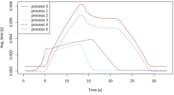
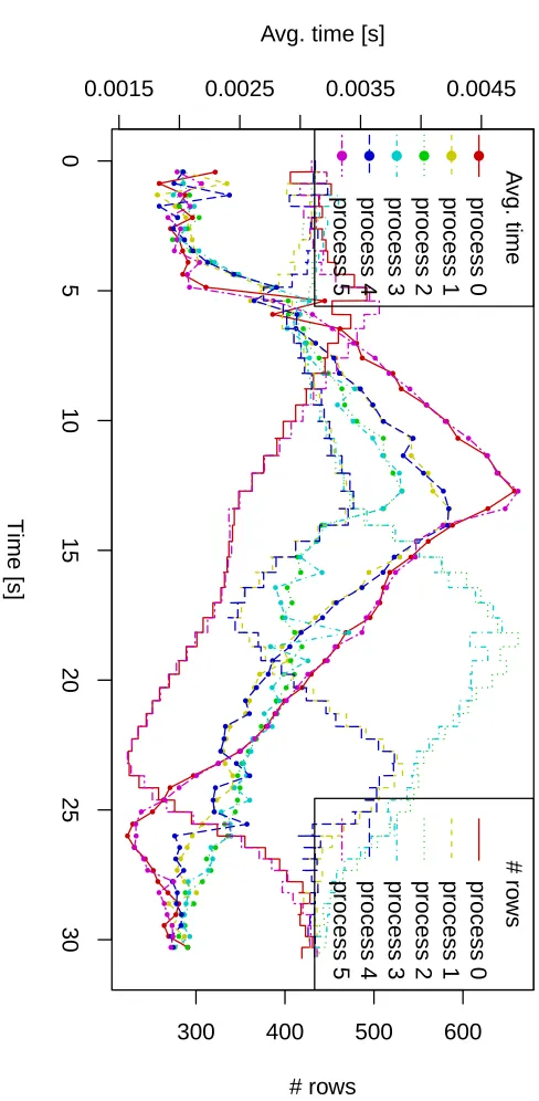
We run the example on Anselm12, a cluster where each node is composed of: two Intel Sandy Bridge E5-2665, 8-core, 2.4GHz processors; 64 GB of physical memory. When the tracing run is complete, we exported the measured data by Kaira and after post-processing in R, we obtained a chart shown in Figure 10. The chart shows that in the middle of the computation, for some processes the computation time of one iteration is more than five times bigger in comparison to other processes. Changing computational times of iterations is caused by spreading non-zero elements in the grid. Therefore, when load balancing is involved, it actively distributes rows between processes. The behavior of the program with active load balancing is shown in Figure 11. It was again obtained in the same way as in the previous case, by exporting the tracelog and post-processed in R. The results indicate that load balancing works in the expected way; slower processes are disposing rows and the average times for a single iteration are more balanced (dotted line are closer together) than without load balancing.
12
Fig. 8.The configuration of the simulated run. The full picture of the net is in Figure 3.
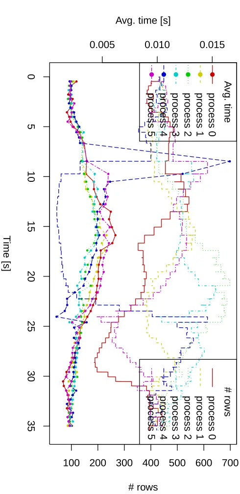
However, the described process allows us to see only the behavior that is reproducible on our currently available hardware. The prediction environment can be used to predict the behavior of the algorithm under more extreme conditions. Let us assume, that we want to see the behavior when a process suddenly becomes much slower and then slowly returns to its original speed. More precisely, after seven seconds of computing, process 4 becomes twelve times slower for another seven seconds and then it uniformly decreases average computational time for another ten seconds. After that it returns to the original speed. Because of simulation, we only need one CPU of the original computer to perform the experiment.
Fig. 9. The tracing configuration for the net of the heat flow with load balancing. Function
rows count returns the number of rows in a grid. The new place at the bottom of the figure is an extra place for tracing the computation times of iterations.
0 5 10 15 20 25 30
0.002
0.003
0.004
0.005
0.006
Time [s]
A
vg. time [s]
process 0 process 1 process 2 process 3 process 4 process 5
Fig. 10.The average computation times of iterations in the heat flow example without load balancing (6 processes;2600×2600; 6000 iterations).
In this example, the clock is started at the beginning of a transition execution and stopped at the end of the computation; therefore the measured time almost exactly matches the full time of the transition execution. Hence, in this case, the same function can be safely used for both settings.
The result of the experiment is shown in Figure 12. After seven seconds of tations, process 4 suddenly slows down, and hence we see in the record that the compu-tational time of an iteration is strongly increased. It is balanced in next three seconds by disposing almost all rows to neighbors. When the execution time is returned to normal, the time of iteration decreases and the rows are gradually returned to process 4.
This demonstration shows that the user can test developed programs in various situa-tions just by changing a simple C++ expression and easily obtain results due to the tracing framework.
6.
Conclusion
informa-0 5 10 15 20 25 30
0.0015 0.0025 0.0035 0.0045
Time [s]
Avg. time [s]
● ● ● ● ● ● ● ● ● ● ● ● ● ● ● ● ● ● ● ● ● ● ● ● ● ● ● ● ● ● ● ● ● ● ● ● ● ● ● ● ● ● ● ● ● ● ● ● ● ● ● ● ● ● ● ● ● ● ● ● ● ● ● ● ● ● ● ● ● ● ● ● ● ● ● ● ● ● ● ● ● ● ● ● ● ● ● ● ● ● ● ● ● ● ● ● ● ● ● ● ● ● ● ● ● ● ● ● ● ● ● ● ● ● ● ● ● ● ● ● ● ● ● ● ● ● ● ● ● ● ● ● ● ● ● ● ● ● ● ● ● ● ● ● ● ● ● ● ● ● ● ● ● ● ● ● ● ● ● ● ● ● ● ● ● ● ● ● ● ● ● ● ● ● ● ● ● ● ● ● ● ● ● ● ● ● ● ● ● ● ● ● ● ● ● ● ● ● ● ● ● ● ● ● ● ● ● ● ● ● ● ● ● ● ● ● ● ● ● ● ● ● ● ● ● ● ● ● ● ● ● ● ● ● ● ● ● ● ● ● ● ● ● ● ● ● ● ● ● ● ● ● ● ● ● ● ● ● ● ● ● ● ● ● ● ● ● ● ● ● ● ● ● ● ● ● ● ● ● ● ● ● ● ● ● ● ● ● ● ● ● ● ● ● ● ● ● ● ● ● ● ● ● ● ● ● ● ● ● ● ● ● ● ● ● ● ● ● ● ● ● ● ● ● ● ● ● ● ● ● ● ● ● ● ● ● ● ● ● ● ● ● ● ● ● ● ● ● ● ● ● ● ● ●
300 400 500 600
# rows # ro ws process 0 process 1 process 2 process 3 process 4 process 5 ● ● ● ● ● ● A vg. time process 0 process 1 process 2 process 3 process 4 process 5
0 5 10 15 20 25 30 35
0.005 0.010 0.015
Time [s]
Avg. time [s]
● ● ● ● ● ● ● ● ● ● ● ● ● ● ● ● ● ● ● ● ● ● ● ● ● ● ● ● ● ● ● ● ● ● ● ● ● ● ● ● ● ● ● ● ● ● ● ● ● ● ● ● ● ● ● ● ● ● ● ● ● ● ● ● ● ● ● ● ● ● ● ● ● ● ● ● ● ● ● ● ● ● ● ● ● ● ● ● ● ● ● ● ● ● ● ● ● ● ● ● ● ● ● ● ● ● ● ● ● ● ● ● ● ● ● ● ● ● ● ● ● ● ● ● ● ● ● ● ● ● ● ● ● ● ● ● ● ● ● ● ● ● ● ● ● ● ● ● ● ● ● ● ● ● ● ● ● ● ● ● ● ● ● ● ● ● ● ● ● ● ● ● ● ● ● ● ● ● ● ● ● ● ● ● ● ● ● ● ● ● ● ● ● ● ● ● ● ● ● ● ● ● ● ● ● ● ● ● ● ● ● ● ● ● ● ● ● ● ● ● ● ● ● ● ● ● ● ● ● ● ● ● ● ● ● ● ● ● ● ● ● ● ● ● ● ● ● ● ● ● ● ● ● ● ● ● ● ● ● ● ● ● ● ● ● ● ● ● ● ● ● ● ● ● ● ● ● ● ● ● ● ● ● ● ● ● ● ● ● ● ● ● ● ● ● ● ● ● ● ● ● ● ● ● ● ● ● ● ● ● ● ● ● ● ● ● ● ● ● ● ● ● ● ● ● ● ● ● ● ● ● ● ● ● ● ● ● ● ● ● ● ● ● ● ● ● ● ● ● ● ● ● ● ●
100 200 300 400 500 600 700
# rows # ro ws process 0 process 1 process 2 process 3 process 4 process 5 ● ● ● ● ● ● A vg. time process 0 process 1 process 2 process 3 process 4 process 5
Listing 1.3.The function used in configurations of time and clock substitutions for the experiment with load balancing of heat flow
ca::IntTime experiment_time(casr::Context &ctx,
ca::IntTime time) {
if (ctx.process_id() == 4) {
if (ctx.time() > 7e9 && ctx.time() < 14e9) {
return time * 12;
}
if (ctx.time() >= 14e9 && ctx.time() < 24e9) {
return (time * (24e9 - ctx.time()) * 12.0) / 10e9;
}
}
return time; }
tion between analysis and debugging, and they allowed us to implement the deterministic replay.
Also for tracing of applications, we use a similar approach and the original model. It is used to present obtained data (application’s replay) and also to simplify measure-ment specifications. This is crucial for tracing, because when we measure everything, the obtained data are usually useless.
The proposed tool offers predictions of application behaviors through online simula-tions with an analytical model of the network. The used model allows simple configura-tion of predicconfigura-tions and observaconfigura-tions of results. During predicconfigura-tions, the complete tracing infrastructure is available. It can be used to check various “what if . . . ” scenarios.
Currently, our tool is not widely used. It is freely available, but we are not aware of other users beside people who are involved in Kaira development. But features de-scribed in this paper are ready to use. We have verified ideas and functionality on various examples together with experimenting with resulting applications on Anselm – the super-computer owned by IT4Innovations Center of Excellence13.
We are also working on new features, the most notable is verification. Again, we want to interconnect it with our model and its’ results (along with results from other analyses) can be used in the remaining Kaira infrastructure. It can serve as another argument why to use Kaira as a prototyping tool for MPI applications.
Acknowledgments.The work is partially supported by GA ˇCR P202/11/0340 and the IT4Innovations Centre of Excellence project (CZ.1.05/1.1.00/02.0070), funded by the European Regional Devel-opment Fund and the national budget of the Czech Republic via the Research and DevelDevel-opment for Innovations Operational Programme, as well as Czech Ministry of Education, Youth and Sports via the project Large Research, Development and Innovations Infrastructures (LM2011033) and by the project SPOMECH – Creating a multidisciplinary R&D team for reliable solution of me-chanical problems, reg. no. CZ.1.07/2.3.00/20.0070 within Operational Programme ‘Education for
13
competitiveness’ funded by Structural Funds of the European Union and state budget of the Czech Republic.
References
1. Allan, R., Science, Britain), T.F.C.G.: Survey of HPC Performance Modelling and Prediction Tools. Technical report (Science and Technology Facilities Council (Great Britain))), Science and Technology Facilities Council (2010), http://books.google.cz/books?id= oirYgEACAAJ 2. B¨ohm, S.: Unifying Framework For Development of Message-Passing
Applica-tions. Ph.D. thesis, FEI V ˇSB-TUO Ostrava, 17. listopadu 15, Ostrava (11 2013), http://verif.cs.vsb.cz/sb/thesis.pdf
3. B¨ohm, S., Bˇeh´alek, M.: Generating parallel applications from models based on Petri nets. Ad-vances in Electrical and Electronic Engineering 10(1) (2012)
4. B¨ohm, S., Bˇeh´alek, M.: Usage of Petri nets for high performance computing. In: Proceedings of the 1st ACM SIGPLAN workshop on Functional high-performance computing. pp. 37–48. FHPC ’12, ACM, New York, NY, USA (2012), http://doi.acm.org/10.1145/2364474.2364481 5. B¨ohm, S., Bˇeh´alek, M., Meca, O., ˇSurkovsk, M.: Visual programming of MPI applications:
Debugging and performance analysis. In: The 4th Workshop on Advances in Programming Language (WAPL) (2013)
6. Casanova, H., Legrand, A., Quinson, M.: Simgrid: A generic framework for large-scale dis-tributed experiments. In: Proceedings of the Tenth International Conference on Computer Mod-eling and Simulation. pp. 126–131. UKSIM ’08, IEEE Computer Society, Washington, DC, USA (2008), http://dx.doi.org/10.1109/UKSIM.2008.28
7. Geimer, M., Wolf, F., Wylie, B.J.N., ´Abrah´am, E., Becker, D., Mohr, B.: The Scalasca per-formance toolset architecture. Concurrency and Computation: Practice and Experience 22(6), 702–719 (Apr 2010)
8. Geimer, M., Wolf, F., Wylie, B.J.N., Mohr, B.: A scalable tool architecture for diagnosing wait states in massively parallel applications. Parallel Comput. 35(7), 375–388 (Jul 2009), http://dx.doi.org/10.1016/j.parco.2009.02.003
9. Hermanns, M.A., Geimer, M., Wolf, F., Wylie, B.J.N.: Verifying causality between distant per-formance phenomena in large-scale mpi applications. In: Parallel, Distributed and Network-based Processing, 2009 17th Euromicro International Conference on. pp. 78–84 (2009) 10. Jensen, K., Kristensen, L.M.: Coloured Petri Nets - Modelling and Validation of Concurrent
Systems. Springer (2009)
11. Kerbyson, D.J., Alme, H.J., Hoisie, A., Petrini, F., Wasserman, H.J., Gittings, M.: Predictive performance and scalability modeling of a large-scale application. In: SC. p. 37 (2001) 12. Knpfer, A., Brunst, H., Doleschal, J., Jurenz, M., Lieber, M., Mickler, H., Mller, M., Nagel, W.:
The Vampir performance analysis tool-set. In: Resch, M., Keller, R., Himmler, V., Krammer, B., Schulz, A. (eds.) Tools for High Performance Computing, pp. 139–155. Springer Berlin Heidelberg (2008), http://dx.doi.org/10.1007/978-3-540-68564-7 9
13. Penoff, B., Wagner, A., Txen, M., Rngeler, I.: MPI-NetSim: A network simulation module for MPI. In: Proc. of the 15th International Conference on Parallel and Distributed Systems (2009) 14. Pillet, V., Pillet, V., Labarta, J., Cortes, T., Cortes, T., Girona, S., Girona, S., Computadors, D.D.D.: Paraver: A tool to visualize and analyze parallel code. Tech. rep., In WoTUG-18 (1995) 15. Pllana, S., Brandic, I., Benkner, S.: Performance modeling and prediction of parallel and
dis-tributed computing systems: A survey of the state of the art. In: CISIS. pp. 279–284 (2007) 16. Shende, S.S., Malony, A.D.: The tau parallel performance system. Int. J. High Perform.
Com-put. Appl. 20(2), 287–311 (May 2006), http://dx.doi.org/10.1177/1094342006064482 17. Squyres, J.M.: Mpi debugging – can you hear me now? ClusterWorld Magazine, MPI Mechanic
18. Squyres, J.M.: Debugging in parallel (in parallel). ClusterWorld Magazine, MPI Mechanic Col-umn 3(1), 34–37 (January 2005), http://cw.squyres.com/
19. Tikir, M., Laurenzano, M., Carrington, L., Snavely, A.: Psins: An open source event tracer and execution simulator for mpi applications. In: Sips, H., Epema, D., Lin, H.X. (eds.) Euro-Par 2009 Euro-Parallel Processing, Lecture Notes in Computer Science, vol. 5704, pp. 135–148. Springer Berlin Heidelberg (2009), http://dx.doi.org/10.1007/978-3-642-03869-3 16
20. Zhai, J., Chen, W., Zheng, W.: Phantom: predicting performance of parallel applications on large-scale parallel machines using a single node. SIGPLAN Not. 45(5), 305–314 (Jan 2010), http://doi.acm.org/10.1145/1837853.1693493
21. Zheng, G., Wilmarth, T., Jagadishprasad, P., Kal´e, L.V.: Simulation-based performance pre-diction for large parallel machines. Int. J. Parallel Program. 33(2), 183–207 (Jun 2005), http://dx.doi.org/10.1007/s10766-005-3582-6
Stanislav B¨ohm is a junior researcher at IT4I - National Supercomputing Center. He finished his Ph.D. study in 2014. His research topics cover programming and formal veri-fication of parallel applications, and complexity of problems in automata theory. He is the leader of the group developing tool Kaira.
Marek Bˇeh´alekis an Assistant Professor in Department of Computer science in V ˇSB Technical University Ostrava. He is also a junior researcher in IT4I National Supercom-puting Center. His research interests are the evolution of programming languages and tools especially for programming of parallel/distributed systems. Now, he is focused on visual programming of distributed applications, their analyzing and verifications.
Ondˇrej Mecahas a diploma degree in computer science from V ˇSB-Technical University of Ostrava. After graduation he started to study doctoral degree at the same university. His research topics cover high performance computing and verification of parallel appli-cations.
Martin ˇSurkovsk´yis a PhD student at V ˇSB - Technical University of Ostrava. He got his master’s degree in computer science at the same university in 2012. His main points of interests are high performance computing and analyses of parallel programs.