A KLEINIAN APPROACH TO FUNDAMENTAL REGIONS

(1)

CSUSB ScholarWorks

Electronic Theses, Projects, and Dissertations Office of Graduate Studies

6-2014

Joshua L. Hidalgo Joshua L Hidalgo

Follow this and additional works at: https://scholarworks.lib.csusb.edu/etd

Part of the Algebraic Geometry Commons, and the Geometry and Topology Commons

Recommended Citation Recommended Citation

Hidalgo, Joshua L., "A KLEINIAN APPROACH TO FUNDAMENTAL REGIONS" (2014). Electronic Theses, Projects, and Dissertations. 35.

https://scholarworks.lib.csusb.edu/etd/35

(2)

A Thesis

Presented to the

Faculty of

California State University,

San Bernardino

In Partial Fulfillment

of the Requirements for the Degree

Master of Arts

in

Mathematics

by

Joshua Lee Hidalgo

(3)

A Thesis

Presented to the

Faculty of

California State University,

San Bernardino

by

Joshua Lee Hidalgo

June 2014

Approved by:

Rolland Trapp, Committee Chair Date

John Sarli, Committee Member

Corey Dunn, Committee Member

Peter Williams, Chair, Charles Stanton

Department of Mathematics Graduate Coordinator,

(4)

Abstract

This thesis takes a Kleinian approach to hyperbolic geometry in order to illus-trate the importance of discrete subgroups and their fundamental domains (fundamental regions). A brief history of Euclids Parallel Postulate and its relation to the discovery of hyperbolic geometry be given first. We will explore two models of hyperbolic n-space:

Un and Bn. Points, lines, distances, and spheres of these two models will be defined and examples in U2, U3, and B2 will be given. We will then discuss the isometries of

(5)

Acknowledgements

(6)

List of Figures

1.1 Euclid’s Parallel Postulate: Playfair’s Axiom . . . 1

1.2 Hyperbolic Parallel Axiom . . . 2

2.1 Point ofU2 . . . 4

2.2 Point ofU3 . . . 4

2.3 Parametrized Curve inU2 . . . 5

2.4 Hyperbolic Lines/Geodesics ofU2 . . . 6

2.5 Hyperbolic Parallele Axiom inU2 . . . 7

2.6 Hyperbolic Planes/Geodesics ofU3 . . . 7

2.7 Hyperbolic Sphere ofU2 _{. . . .} ₈

2.8 Hyperbolic Sphere ofU3 . . . 8

2.9 Horosphere ofU2 . . . 9

2.10 Horosphere ofU2 _{. . . .} ₁₀

2.11 Point ofB2 . . . 11

2.12 Non-Euclidean Distance ofB2 . . . 11

2.13 Hyperbolic Lines/Geodesics ofB2 _{. . . .} ₁₂

2.14 Hyperbolic Parallele Axiom inB2 . . . 13

2.15 Hyperbolic Sphere of B2 . . . 13

2.16 Horocycle ofB2 _{. . . .} ₁₄

3.1 Hyperplane ofE2 . . . 16

3.2 Hyperplane ofE3 . . . 16

3.3 Reflection in a Hyperplane . . . 17

3.4 Reflection in a General Hyperplane ofE3 . . . 17

3.5 Inversion in a circleC . . . 18

3.6 Inversions ofU2 . . . 19

3.7 M¨obius Transformation,φ, of U2 . . . 20

3.8 Inversions ofB2 . . . 21

3.9 M¨obius Transformation,φ, of B2 . . . 22

3.10 Parabolic Transformation of U2 . . . 23

3.11 Parabolic Transformation of B2 . . . 24

3.12 Hyperbolic Transformation of U2 . . . 24

(8)

3.14 Fixed Points of a Hyperbolic Transformation of B2 . . . 25

3.15 Elliptic Transformation ofU2 . . . 25

3.16 Elliptic Transformation ofB2 _{. . . .} ₂₆

4.1 Orbit ofU2 . . . 30

4.2 Discontinuous Group Action . . . 31

5.1 Fundamental Domain,R . . . 33

5.2 Mutually DisjointgR for allg∈Γ . . . 33

5.3 U2=∪gR¯ for all g∈Γ . . . 34

5.4 Fundamental Region,R . . . 34

5.5 Mutually DisjointgR for allg∈Γ,R as a Fundamental Region . . . 35

5.6 U2=∪gR¯ for all g∈Γ,R as a Fundamental Region . . . 35

5.7 Ideal Hyperbolic Square . . . 37

5.8 Orbit ofiin the Ideal Hyperbolic Square . . . 37

5.9 Perpendicular Bisectors of [i, φ(i)] . . . 37

5.10 Dirichlet Domain,D(i) . . . 38

5.11 Lattice of points inE2 . . . 39

5.12 Euclidean Torus, X/Γ . . . 40

5.13 Euclidean Punctured Torus . . . 40

5.14 Hyperbolic Punctured Torus . . . 41

(9)

Chapter 1

Introduction

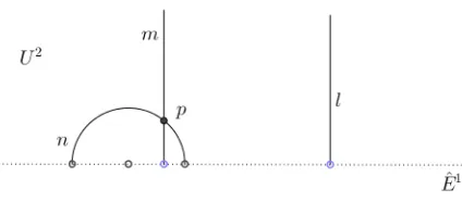
Euclid’s Parallel Postulate is historically one of the most researched and studied writings of mathematics. Mathematicians tried proving this particular postulate and have failed over the years. Euclid himself used it very sparingly in proving various theorems in his book, Elements. This is because, unlike Euclid’s other postulates, the Parallel Postulate cannot be proved using his other axioms. Of all the equivalent statements of the Parallel Postulate, Playfair’s axiom, named after the Scottish mathematician John Playfair, is probably the most well-known. It essentially states that given any straight line land a point p not onl, there exists a unique straight line m which passes through

p and never intersectsl, no matter how far they are extended. As shown in Figure 1.1. Let us analyze Playfair’s version of Euclid’s Parallel Postulate. The postulate gives two

Figure 1.1: Euclid’s Parallel Postulate: Playfair’s Axiom

interesting claims: one is that parallel lines exist and the other is that the parallel line is unique. These two claims are crucial to Euclidean geometry and Euclidean n-space,

(10)

one line, say nand m, throughp that do not intersectl. Implying that the parallel line through p is no longer unique.

Figure 1.2: Hyperbolic Parallel Axiom

The subject of hyperbolic geometry was fine-tuned in the 19th _{century and expanded on}

(11)

Chapter 2

Models of Hyperbolic Space

In this chapter, we will look at hyperbolic geometry and how it can be studied using two common models: the open upper-half-space, Un_{, and open ball,}_Bn_{. A model}

for hyperbolic geometry is a definition of points, lines, and distances that satisfies the axioms. In particular, the hyperbolic parallel axiom is satisfied in each of these models. (Throughout this chapter we cite [Bon09], [Bra99], and [Rat94].)

2.1

Open Upper-Half-Space Model,

U

n

In this section we describe the open upper-half-space,Un, and how its Euclidean properties can be used to describe hyperbolic geometry. We will be looking at points, metric, ideal points, lines, planes,andspheres ofUn. Examples inU2andU3and familiar subsets of Euclidean space will help us describe these properties of Un. Points inUn can be described using real or complex numbers. Upper half-space is generally defined in the following way:

Un={(x1, x2, . . . , xn)∈En|xn>0}.

We can identify the upper half-plane, U2, as the set

{z∈C|Imz >0}.

The upper half-space,U3, can be defined as the set of quaternions

(12)

or more commonly

{q=a+bi+cj|a, b, c∈Rand c >0}

where i2 =j2 =−1.

Example 2.1.1. In U2_,_a₌_i_.

Figure 2.1: Point of U2

N

Example 2.1.2. In U3_,_a₌_i₊_j_.

(13)

Now lets look at some of representations of the metric for Un,dU. One metric

is given by

coshdU(x, y) = 1 +

|x−y|2

2xnyn

,

where |x−y| is the standard Euclidean distance, dE. It is known that hyperbolic arc

length of a curveγ is different from Euclidean arc length. ForUn_{, it is are given by the}

formula

|dx| xn

.

In U2, this definition implies arc length can be calculated as follows. Let γ be the differentiable vector valued function

t7→ x(t), y(t), such thata≤t≤b.

Then

l_U2(γ) =

Z b

a

p

x0(t)2₊_y0₍_t₎2 y(t) dt.

This metric provides a way to measure lengths of curves. We will illustrate this with an example.

Example 2.1.3. Suppose γ is parametrized by

t7→(0, t), such that a≤t≤b,

as shown in the following figure.

(14)

Then

l_U2(γ) =

Z b

a

p

(0)2_{+ (1)}2

t dt=

Z b

a

1

tdt= ln(b)−ln(a) = ln

b a . N

Before we talk about what lines look like in Un, we will first look what what it means to be an ideal point. Generally, ideal points are points at infinity that are not included in the space but may be included in its Euclidean closure. We can think of these ideal points as ˆEn−1 = En−1∪ {∞}, where ˆEn =En∪ {∞} is the extended Euclidean plane. These points have special properties that may effect points in the space. In U2,

ideal points are the real line (or the x-axis) and the point at infinity. Now we will look athyperbolic lines inUn and how they differ from Euclidean lines.

Definition 2.1.4. Hyperbolic lines ofUn are geodesics of Un.

The following examples show hyperbolic lines, geodesics, inU2 and U3. There are two types: Euclidean semicircles (semispheres) centered on the real line (plane) or Euclidean vertical rays (planes) originating on the real line (plane). If we think of vertial rays (planes) as semicircles (semispheres) centered at ∞, then all hyperbolic lines are in fact semicircles (semispheres) centered at an ideal point.

Example 2.1.5. In U2, let l1={z=eiθ |0< θ < π} and l2={x= 4|y >0}.

(15)

Note, with this definition of a hyperbolic line, that the hyperbolic parallel axiom is satisfied. Both lines nand m through p do not intersect to the linel.

Figure 2.5: Hyperbolic Parallele Axiom in U2

Example 2.1.6. Planes in U3, let l1 = {(1, θ, φ) | 0 < θ ≤ 2π and 0 ≤ φ < π

2} and

l2 ={(x1,4, x3)|x1∈Rand x3 >0}. See figure 2.5 below.

Figure 2.6: Hyperbolic Planes/Geodesics of U3

N

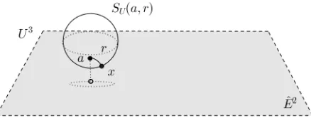
Now that we have looked at hyperbolic lines in Un, lets take a look at spheres (circles) inUn.

Definition 2.1.7. Thehyperbolic sphere ofUn, with centeraand radiusr >0, is defined to be the set

(16)

This is shown inU2 in the following example. Take note that every hyperbolic sphere of U2 is a Euclidean circle in U2, though the hyperbolic radius and hyperbolic center are different from the Euclidean radius and the Euclidean center of the circle.

Example 2.1.8. In U2, let SU(2 + 2i,1) ={x∈U2:dU(2 + 2i, x) = 1}.

Figure 2.7: Hyperbolic Sphere ofU2

N

Example 2.1.9. In U3, let SU(2i+ 2j,1) ={x∈U3:dU(2i+ 2j, x) = 1}.

(17)

Lastly we will look athorospheres ofUn and look at what they may look like in

U2 and U3.

Definition 2.1.10. Let b be an ideal point of U2. Horospheres are Euclidean spheres tangent, at b, to ˆEn−1 or horizontal planes (whenbis at∞) in Un. The point bis called the “center” of thehorosphere.

In U2 and U3, horospheres are shown as Euclidean circles (spheres) tangent to the real axis (plane) and Euclidean lines (planes) parallel to the real axis (plane), this is actually a sphere centered at∞, respectively. It is important to note that the pointb, as described in the definition, is not in the open half-space but is in the set of ideal points of the open half-space. In the Eucliden sense, b is on the sphere. So the hyperbolic center of a horosphere is very different from the Euclidean center.

Example 2.1.11. InU2_,_S

1 =x+ 3i(a circle with center at ∞) and S2= (i,1) ={x∈ U2 :dE(i, x) = 1}.

Figure 2.9: Horosphere ofU2

N

Example 2.1.12. InU3,S1 = 2j (a sphere with center at∞) andS2 = (i+j,1) ={x∈ U3 :dE(i+j, x) = 1}.See Figure 2.10.

(18)

Figure 2.10: Horosphere ofU2

2.2

Open-Ball Model,

B

n

This subsection will focus on our second representation ofHyperbolic Geometry, the open-ballBn. Similar toUn,Bn, can be described using familiar Euclidean properties. We will again look at points, metrics, ideal points, lines, planes, and spheres of Bn. Examples of these properties will be shown using B2 and familiar subsets of Euclidean space. Let us first look at points in Bn. Let Bn be the unit open-ball in Euclidean n-space, so that

Bn={x∈En| |x|<1}.

We will look at B2 for our examples. We can define B2 to be the unit disk. The unit disk can be represented in two ways, both having their advantages:

{z| |z|<1}

or

{(x, y)|x2+y2<1}.

Example 2.2.1. In B2,a= i

2. See Figure 2.11.

N

(19)

Figure 2.11: Point ofB2

where |x−y| again is the standard Euclidean distance. Similar to Un, hyperbolic arc length of a curve γ in Bn _{is different from Euclidean arc length. For} _Bn_{, it is are given}

by the formula

2|dx|

1− |x|2.

In B2, the hyperbolic distance between two pointsz1 andz2 is defined by

dB(z1, z2) = tanh−1

z2−z1

1−z¯1z2

.

Example 2.2.2. Let a= 1

3iand b= 1

2. Then

Figure 2.12: Non-Euclidean Distance ofB2

d(b, a) =d 1

2, 1 3i

= tanh−1

1 2− 1 3i

1−1₃i·1₂

≈0.6819.

(20)

It is worth mentioning that above metric and the spaceBncreates theconformal ball model ofHn. Since the model is conformal, angles inBn are the same as Euclidean angles. In other words, the angle between two geodesic rays is the Euclidean angle between the tangents to the rays. Now for Bn,ideal points are on the boundary of Bn. Next let us take a look at hyperbolic lines ofBn. We have a simililar definition ofhyperbolic lines

of Bn as we do inUn.

Definition 2.2.3. Hyperbolic lines ofBn are geodesics ofBn.

These are either arcs of circles orthogonal to the unit circle or diameters ofB2. If the line is a diameter of B2_{, then this is just an arc of a generalized circle with the}

center at the point of infinity. In this model, each hyperbolic line is part of a Euclidean generalized circle which is orthogonal to the boundary ofBnand are inBn. The following example gives two images of these geodesics inB2.

Example 2.2.4. InB2, Letl1 ={(x, y)TB2 |y=x} and l2={(x, y)TB2 |x2+y2−

4x+ 1 = 0}.

Figure 2.13: Hyperbolic Lines/Geodesics of B2

N

(21)

Figure 2.14: Hyperbolic Parallele Axiom inB2

Next, we will look at hyperbolic spheres of Bn. Similar to how we examined spheres ofUn,hyperbolic spheres ofBnare Euclidean spheres, only with different centers and radii.

Definition 2.2.5. Thehyperbolic sphere ofBnwith centeraand radiusr >0, is defined to be the set

SB(a, r) ={x∈Bn|dB(a, x) =r}.

The following example shows this in B2.

Example 2.2.6. In B2_{, Let}_S ₌ 1 2 +

1 2i,

1 4

= {x ∈B2 _|_d

B 1₂ +1₂i, x

= 1₄}. Observe once again, S is also an Euclidean circle just with different center and radius.

(22)

N

This section will end with the definition and an example of horospheres of Bn. The example will be given in B2.

Definition 2.2.7. Ahorosphere centered atb∈Sn−1 is an Euclidean sphere tangent, at

b, toSn−1 inBn.

Example 2.2.8. A horosphere is sometimes called a horocycle when in two dimensions. Here, in B2, the horocycle S is tanget to the boundary of B2 at

√

2 2 ,

√

2 2 i

.

Figure 2.16: Horocycle ofB2

(23)

Chapter 3

Isometries of

U

n

and

B

n

Christian Felix Klein (1849-1926) was a German mathematician who introduced a new take on geometry and how different geometries could be classified. His work in the 1870’s allows us to approach a geometry not as a set of axioms, and their consequences, but as a space together with a group of transformations acting on the space. Any properties remaining invariant by the group transformations would become the geometric properties of that space. If a transformation is not changing the properties of the shapes in the space, then we might be looking at the group of isometries of that space. It was Kleins view that connected the mathematics of group theory and geometry. This is the approach we will take while studying the metric spaces Un andBn. In this section we will investigate

inversions, the group of M¨obius transformations, and their relationship to hyperbolic geometry by looking at examples inU2andB2. (Throughout this chapter we cite [Bon09], [Bra99], and [Rat94].)

3.1

Inversion

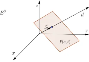
Before talking aboutM¨obius transformations, it is important to learn about the type of transformation known asinversion. In summary,inversion is areflection in a line or a circle. These inversions map points from one side of a sphere of ˆEn to the other. Let us first look at hyperplanes of En defined as (n−1)-planes ofEn such that

(24)

In this definition,~ais a unit vector inEn, which is normal toP(a, t). Moreover, tis the scalar multiple of a that lies on P(a, t). The following two examples give us a visual of hyperplanes of E2 _and _E3_{, respectively.}

Example 3.1.1. LetP be the hyperplaneP(h1,0i,2) ={(x, y)∈E2 | h1,0i · hx, yi= 2}

inE2.

Figure 3.1: Hyperplane of E2

N

Example 3.1.2. Let P be the general hyperplaneP(a, t) in E3.

(25)

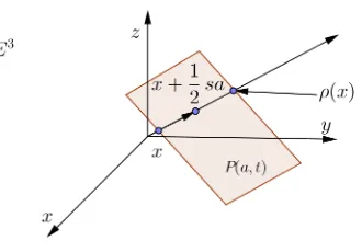
Now that we know what a hyperplane is, lets look at areflection in a hyperplane. These reflections turn out to be Euclidean reflections as we all know them! These next two examples are reflections in hyperplanes ofE2 _and _E3_{, respectively.}

Example 3.1.3. Let P be the hyperplaneP(h1,0i,2) in E2 and ρ(x) be the reflection of x inP(h1,0i,2).

Figure 3.3: Reflection in a Hyperplane

N

Example 3.1.4. Let P be the general hyperplane P(a, t) inE3 and ρ be the reflection of x inP(a, t)

Figure 3.4: Reflection in a General Hyperplane ofE3

(26)

Generally, we will define areflection ρ ofEnin the planeP(a, t) by the formula

ρ(x) =x+ (t−a·x)a.

As mentioned above, inversions are reflections in lines or circles. Up until now we have only taken a look at reflections in a line (or hyperplane). Now let us take a look at

inversions in a Euclidean circle. Let C be a circle with center O and radius r, and let A be any point other than O. If A0 is on the ray −→OA and satisfies the equation

OA·OA0 =r2, then we call A0 the inverse of A with respect to the circle C where C is the circle of inversion. The transformation

σ(A) =A0

is known as inversion inC.

Figure 3.5: Inversion in a circleC

Suppose we have the sphereS(a, r) ofEnsuch thatS(a, r) ={x∈En| |x−a|=

r}, then we will use the following formula for inversion in a sphere:

σ(x) =a+ r

|x−a|

!2

(x−a).

The term inversion will now mean either reflection in a hyperplane or inversion in a sphere. We will now give an example showing two inversions in U2.

Example 3.1.5. Letσ1 be the inversion inl1 and σ2 be the inversion inl2. See Figure

3.6. Notice that the inversion in l1 sends points within the arc to points outside the arc

(27)

Figure 3.6: Inversions of U2

3.2

M¨

obius Transformations of

U

n

In this section we will investigate Möbius transformations of Un by looking at examples in U2_{. We will also look at the algebraic properties of these} _M¨_obius transfor-maitons in this space. First let us define a sphere of Σ of Ên to be either a Euclidean sphere S(a, r) or an extended plane ˆP(a, t) =P(a, t)∪ ∞. Note that ˆP(a, t) is topologi-cally a sphere. We will first define a Möbius transformation.

Definition 3.2.1. A M¨obius transformation of ˆEn is a finite composition ofinversions

of ˆEn _{in spheres.}

It turns out Möbius transformations of Un are Möbius transformations of Ên

that leave Un unchanged. If we use the complex definition ofU2, these M¨obius transfor-mations turn out to be isometries of U2 known as linear fractional transformations.

Theorem 3.2.2. The isometries of the U2 _{are linear fractional transformations of the} form:

1. φ(z) = az+b

cz+d with a, b, c, d∈R andad−bc= 1,

2. and φ(z) = cz¯+d

az¯+b with a, b, c, d∈Rand ad−bc= 1.

(28)

written as a composition of inversions. Rather than provide a proof, we will illustrate with an example that the composition of two particular inversions result in a linear fractional transformation. Let us take a look at the inversions in Example 3.1.5 and find a M¨obius transformation,φ, such thatφ=σ2◦σ1. First we will assign some values. Let l1 ={z=x+yi | |z|= 1 and y >0}. Then the inversion in l1 is defined as σ1(z) =

1 ¯

z.

Also let l2 ={z= 4 +yi|y >0}. Then the inversion inl2 is defined asσ2(z) =−z¯+ 8.

Now since φ = σ2 ◦σ1, this implies φ(z) =

8z−1

z . Notice that this transformation

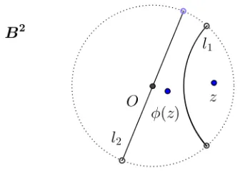
satisfies the definition of linear fractional transformations,ad−bc= (8)(0)−(−1)(1) = 1. The M¨obius tranformation,φ, is shown in the following image.

Figure 3.7: M¨obius Transformation,φ, of U2

3.3

M¨

obius Transformations of

B

n

The linear fractional transformation φ(z) = −z+i

z+i induces an isometry from U2 to B2. This mapping, known as the standard transformation, is useful to take what we know about U2 and find out what it looks like in B2. We will now look at M¨obius transformations of Bn. In this subsection we will investigate M¨obius transformations of

(29)

Example 3.3.1. Let σ1 be the inversion inl1 and σ2 be the inversion in l2.

Figure 3.8: Inversions of B2

N

Now it turns out M¨obius transformations of Bn are M¨obius transformations

of ˆEn that leave Bn unchanged. If we use the complex definition of B2, these M¨obius transformations are also isometries.

Theorem 3.3.2. The isometries of the B2 are linear fractional transformations of the form:

1. φ(z) =_¯az+b

bz+ ¯a with a, b∈C and|a|

2_{− |b|}2 _{= 1}_,

2. and φ(z) =_¯az¯+b

bz¯+ ¯a with a, b∈Cand |a|

2_{− |b|}2 _{= 1}_.

These can be derived by using the mapping φ(z) = −z+i

z+i on the linear

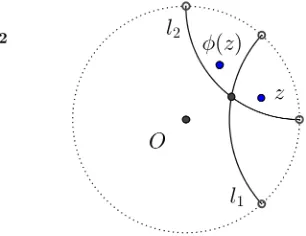
frac-tional transformations of U2. Let us now take a look at the inversions in Example 20 and find a M¨obius transformation, φ, such that φ = σ2 ◦σ1. We will do this in

the same fashion as finding φ in the previous subsection. Let l1 = {(x, y) ∩B2 | −1 < x < 1 and y = 0}. Then the inversion in l1 is defined as σ1(z) = ¯z. Now

let l2 = {(x, y)∩B2 | x2 +y2 −2 √

2 + 1 = 0}. Then the inversion in l2 is defined

as σ2(z) = √

2¯z−1 ¯

z−√2 . Now since φ = σ2 ◦σ1, this implies φ(z) =

√

2z−1

(30)

that this transformation satisfies the definition of linear fractional transformations ofB2,

|√2|2_{− | −}₁_|2_{= 1. The M¨}_{obius tranformation,} _φ_{, is shown in the following image.}

Figure 3.9: M¨obius Transformation,φ, of B2

There are different types of M¨obius transformations. In the next section, we will classify these transformations and explain their properties with examples in U2 and B2.

3.4

Parabolic, Hyperbolic, and Elliptic Transformations

Here, we will look at different M¨obius transformations and the behavior they may have. There are three types of M¨obius transformations: parabolic, hyperbolic, and

elliptic. The difference bewteen these transformations are the number of fixed points and their locations. To help explain, we will observe the M¨obius transformations ofU2. First of all, it is obvious that the identity mapφ(z) =zfixes all the points, but there are other maps that fix other particular points. To find these fixed points we will have to solve the equation

φ(z) = az+b

cz+d =z.

Using the Quadratic Formula, we get the resulting solution:

z= a−d±

p

(d−a)2_{+ 4}_bc

(31)

substition, we have a new form for our determinant: (a+d)2−4. Now we will describe the difference between the three transformations mentioned above. If (a+d)2 = 4 we have a parabolic transformation which gives a unique fixed real number z = a−d

2c . If

(a+d)2 > 4 then we have a hyperbolic transformation giving two real fixed points. If 0 <(a+d)2 < 4 then we have an elliptic transformation which has two complex fixed points. Generally, a transformation is said to be

(1) parabolicifφfixes no points ofUnorBnand fixes a unique point in their boundaries; (2) hyperbolic if φ fixes no points of Un or Bn and fixes two unique points in their

boundaries;

(3) elliptic ifφfixes at least one point of Un orBn.

The rest of this section will demonstrate various M¨obius transformations of bothU2 and

B2.

Example 3.4.1. Letφ(z) =z−4 andz∈R such thatR={z=x+iy|1< x <2, y >

0}. Then φ(z) is as shown below. The transformation φ is parabolic in U2 because it

Figure 3.10: Parabolic Transformation of U2

only fixes the point at infinity.

N

Example 3.4.2. Letφ(z) = (122 + 45i)z+ (−88−60i)

(−88 + 60i)z+ (122−45i). Thenφ(z) is a composition of inversions in l1 and l2 as shown below in Figure 3.11. The transformation φis parabolic

(32)

Figure 3.11: Parabolic Transformation of B2

N

Example 3.4.3. Letφ(z) = 1

2z and z∈R such thatR={re

iθ _|₁_{< r <}₂_,₀_{< θ < π}}_.

Then φ(z) is as shown below in Figure 3.12. The transformation φ is hyperbolic in U2

because it only fixes the point at infinity and the origin.

Figure 3.12: Hyperbolic Transformation of U2

N

Example 3.4.4. Let φ(z)(z) = (91 + 9i)z+ (−63−12i)

(−63 + 12i)z+ (91−9i). Then φ(z) is as shown in Figure 3.13. The transformation φ is hyperbolic in B2 because it fixes two points on the boundary of B2_{. These points turn out to be the end points,} _a_and _b_{, of the unique}

(33)

Figure 3.13: Hyperbolic Transformation ofB2

Figure 3.14: Fixed Points of a Hyperbolic Transformation of B2

Example 3.4.5. Let φ(z) = 1 ¯

z and z ∈R such that R ={re

iθ _|₀_{< r <}₁_,₀ _{< θ < π}}_.

Then φ(z) is as shown in Figure 3.15. The transformation φ is elliptic inU2 because it only fixes fixes the arc of the circle-of-inversion.

Figure 3.15: Elliptic Transformation ofU2

(34)

Example 3.4.6. Let φ(z) = (247 + 174i)z+ (−100−232i)

(−100 + 232i) + (247−174i) . Then φ(z) is as shown below in Figure 3.16. The transformation φ is elliptic in B2 because it only fixes the point at which l1 and l2 intersect.

Figure 3.16: Elliptic Transformation ofB2

(35)

Chapter 4

Topogical Groups

In this chapter we will study a bit abouttopological groups and their structures related to hyperbolic n-space. We will also look into discrete groups and discontinuous groups. This chapter will definitely prepare us to think about geometry in the same way Klein did, a group acting on a space. In Chapter 1 we described two models of hyperbolic

n-space while Chapter 2 talked about isometries of hyperbolic n-space. We will begin to look at the set of isometries ofHnas a group.( Throughout this chapter we cite [Rat94].)

4.1

Topological Groups

In this section, we will define transformational groups, topological groups, and

quotient topological groups. First let us define a transformational group.

Definition 4.1.1. A transformational group on a set X is a family Γ of bijections γ :

X →X such that

(1) ifγ and γ0 are in Γ, their compostion is also in Γ;

(2) the group Γ contains the identity map IdX;

(3) ifγ is in Γ, its inverse mapγ−1 is also in Γ.

Generally, a set of isometries from a metric space X to itself, together with multiplication defined by composition, froms a groupI(X), called thegroup of isometries

(36)

Definition 4.1.2. A topological group is a groupGthat is also a tolopogical space such that the multiplication (g, h)7→ghand inversiong7→g−1 inGare continuous functions.

Example 4.1.3. The realn-spaceRnwith the operation of vector addition is atopological

group.

N

Example 4.1.4. The complex n-space Cn with the operation of vector addition is a

topological group.

N

Example 4.1.5. The projective special linear group P SL(2,R) is a topological group.

N

It is worth mentioning a few things about quotient topological groups. Suppose

H is a subgroup ofG, a topolocial group. Then the coset spaceG/H ={gH |g∈G} is equiped with the quotient topology. We will define the quotient map by π:G→G/H.

Theorem 4.1.6. If N is a normal subgroup of a topological group G, then G/N, with the quotient topology is a topogical group.

Example 4.1.7. The projective general linear group P GL(n,C) = GL(n,C)/N, where

N is the normal subgroup{kI |k∈_R∗_} _{is a}_{quotient topological group}_.

N

4.2

Discrete Subgroups

The next group that we willl investigate is thediscrete group. We will also define agroup action and a give an example of anorbit inU2. Discrete subgroups of continuous groups will be of particular interest. After defining the discrete group we will provide some examples of discrete subgroups.

(37)

N

Example 4.2.3. Z[i] ={m+ni:m, n∈Z} is a discrete subgroup of C.

N

Example 4.2.4. The modular group P SL(2n,Z) = SL(2n,Z)/{±I} is a descrete sub-group ofP SL(2n,R).

N

Let us now define what it means for a group toact on a set. With this definition we move closer to Klein’s view of geometry as explained in his work.

Definition 4.2.5. A group G acts on a set X if and only if there is a function from

G×X toX, written (g, x)7→gx, such that for allg, h∈Gand x∈X, we have

(1) 1·x=x and

(2) g(hx) = (gh)x.

A function from G×X toX satisfying (1) and (2) is called an aciton of Gon X.

We now essentially have what we need to study Klein’s program: knowledge of groups and actions. Let G be a group acting on a set X and letx ∈ X. We define the following terms:

(1) the subgroup Gx ={g∈G|gx=x} ofG is called thestabalizer ofx∈G;

(2) the subset Gx={gx|g∈G}of X is called theG-orbit through x;

(3) if φ :G/Gx → Gx by φ(gGx) = gx, then φ is a bijection and therefore the index

Gx in G is the cardinality of the orbit Gx. This is in reference to the familiar

Orbit-Stabalizer Theorem.

(38)

Figure 4.1: Orbit of U2

4.3

Discontinuous Groups

Finally we take a look at another interesting type of group: the discontinuous groups. Let us first define a discontinuous action and a homeomorphism.

Definition 4.3.1. A group Γ actsdiscontinuously on a topological space X if and only if Γ acts onX and for each compact subsetK ofX, the setK∩gK is nonempty for only finitely many g in Γ.

The previous action in the last example is discontinuous. In the previous exam-ple, the group hφi acts discontinuously on U2 because we can take a compact subsetK

of U2_{, and there will only be a finite amount of points from the orbit of}_p _in_K_∩_gK_{, for} g ∈ Γ. Any compact subset K of U2 will be closed and bounded. Therefore there will be a maximum and minimum distance from K to (0,0). Let M=maximum distance and

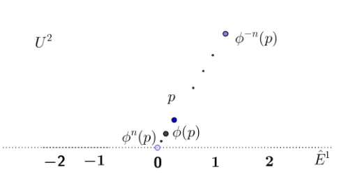
m=minumum distance. As long as 2Nm > M,φN(K) will be farther from (0,0) than K, soφN(K)∩K=φ. Similarly, as long as 2nM < m, we will haveφn(K)∩K=φ. Hence only finitely many elements g inhφihave gK∩K 6=φ. The following example, however, is not of a discontinuous aciton.

Example 4.3.2. Letφ(z) =rz for all r ∈_Rand Γ =hφi be the cyclic group generated by φ. In this case, the orbit of a point p is the ray orginating from the origin throught

(39)

be used again in the next chapter. N

Figure 4.2: Discontinuous Group Action

Definition 4.3.3. Let X and Y be topological spaces; let f :X → Y be bijection. If both the function f and the inverse function f−1 : Y → X are continuous, then f is called ahomeomorphism.

We will can now define what it means to be a discontinuous group.

Definition 4.3.4. A group Gof homeomorphisms of a topological spaceX is discontin-uous if and only if Gacts discontinuously on X.

(40)

Chapter 5

Geometry: Fundamental Regions

We have now come to our final chapter. We will define fundamental regions,

fundamental domains, andDirichlet domains and make relationships between these con-cepts. To help visualize these concepts, examples inU2will be given using familiar points, lines, regions, and actions. We will end by seeing how fundamental domains characterize discrete subgroups of I(U2) and how they can help us visualize group actions of I(U2). Throughout this chapter we cite [Bon09] and [Rat94].

5.1

Fundamental Regions and Fundamental Domains

Let us start by first defining afundamental region.

Definition 5.1.1. A subset R of a metric space X is a fundamental region for a group Γ of isometries of X if and only if

(1) the set R is open inX;

(2) the members of{gR:g∈Γ}are mutually disjoint; and

(3) X =∪{gR¯ :g∈Γ}. Here, ¯R is the closure ofR.

Definition 5.1.2. A subsetDof a metric spaceX is a fundamental domain for a group Γ of isometries of X if and only if Dis a connected fundamental region for Γ.

(41)

Similar to Example 1, we can derive φn₍_z_{) =} 1 2 n z.

Figure 5.1: Fundamental Domain, R

(1) R is open inU2 by the wayR is defined above.

(2) All the members of {gR : g ∈ Γ} are mutually disjoint. This is true since the

boundaries ofRare not inRand Φn(R) is between circles with radius

1 2

n−1

and

1 2

n

We can see this in the following figure.

Figure 5.2: Mutually DisjointgR for all g∈Γ

(3) U2 =∪{gR¯ :g∈Γ}. This is true since the only pieces missing are circles with radii

1 2

n

(42)

Figure 5.3: U2=∪gR¯ for all g∈Γ

2zand Γ = hφi be the group action generated byφin U

2_.

Let R1 ={z =reiθ |1< r < 2, π

2 < θ < π} and R2 ={z=x+iy |1< x < 2, y >0}. Then the region R = R1∪R2 is a fundamental region for Γ. We can derive Φn(z) =

1 2

n

z.

Figure 5.4: Fundamental Region,R

(1) R is open inU2 _{by the way}_R _{is defined above.}

(43)

this in Figure 5.6. N

Figure 5.5: Mutually DisjointgR for all g∈Γ,R as a Fundamental Region

Figure 5.6: U2=∪gR¯ for all g∈Γ,R as a Fundamental Region

Theorem 5.1.5. If a group Γ of isometries of a metric space X has a fundamental region, then Γ is a discrete subgroup of the groups of isometries ofX, I(X).

Proof:Let x be a point of a fundamental region R for a group of isometries Γ of a metric space X. Then the evaluation map

ε: Γ→Γx,

(44)

Γx is trivial, again by the definition of a fundamental region. Now suppose that {1} is

open. Let g be in Γ. Then left multiplication by g is a homeomorphism of Γ. Since homeomorphism’s map open sets to open sets, g{1} = {g} is open in Γ. This implies 1 =ε−1(x) is open in Γ by howεis defined above. Therefore Γ is discrete.

5.2

Dirichlet Domains

Now that we have looked at fundamental regions and fundamental domains, we will study what it means to be a Dirichlet domain. Let Γ be a discontinuous group of isometries of the metric space Hn, and let u be a point of Hn whose stabalizer Γu is

trivial. For each g6= 1∈Γ, define

Hg(u) ={x∈X |d(x, u)< d(x, gu)}.

It turns out, Hg(u) is the open half-space of Hn containing u whose boundary is the

perpendicular bisector of the geodesic segment joining u to gu. The Dirichlet domain D(u) for Γ, withcenter u, is either Hn if Γ is trivial or

D(u) =∩{Hg(u)|g6= 1∈Γ}

if Γ is nontrivial.

Example 5.2.1. Let X be the ideal hyperbolic square below in Figure 5.7. If Γ =

hφ₁(z) = z+ 1

z+ 2, φ2(z) =

z−1

−z+ 2i, then the orbit of i ∈ X generated by Γ is as shown in Figure 5.8. Now by finding all the perpendicular bisectors of the segments [i, φ(i)] for

φ∈Γ (Figure 5.9), we derive the Dirichlet domain, D(i), shown below in Figure 5.10.

N

Theorem 5.2.2. LetD(u)be the Dirichlet domain, with center u, for a discrete subgroup

(45)

Figure 5.7: Ideal Hyperbolic Square

Figure 5.8: Orbit of iin the Ideal Hyperbolic Square

(46)

(47)

5.3

Visualizing Quotient Spaces

Now, using what we know about the quotient topology and group acitons, an informal definition of aquotient space will be given. Let Γ be the topological group acting on a space X. If we say points on X are equivalent if and only if they lie in the same orbit, then X/Γ is thequotient space of X under the action of Γ. Fundamental domains are useful because they allow us to intuitively visualize X/Γ. The following examples are of well known fundamental domains: the torus (using E2) and the punctured torus (using U2).

Example 5.3.1. First, letX =E2 _{and Γ be the subgroup of}_I₍_E2_{) consisting of}

trans-lations by vectors with integral components. In other words, let

φm,n :E2→E2

be defined by

φm,n: (x, y)→(x+m, y+n),

then Γ =hφ_m,niwherem, n∈_Z. The orbit of (0,0) under the action of Γ is the “lattice”

{(m, n) |m, n ∈ _R}, shown below in Figure 5.11. Similarly, the orbit of any point will

Figure 5.11: Lattice of points inE2

(48)

with (m, n) as the lower left corner. NowR is open inX andR∩gRis the empty for all

g∈Γ that are not the identity satisfying properties (1) and (2) of fundamental domains, and ¯R is the closed unit square and tesselates X. So x=∪gR¯ satisfying property (3) of fundamental domains. Thus, the quotient space X/Γ can be visualized in the following way:

Figure 5.12: Euclidean Torus, X/Γ

N

Suppose the orbit of (0,0) in X in the above example is not included. Then

X/Γ becomes the punctured torus below in Figure 2.13. Topologically, this is the same as the punctured torus in the next example.

(49)

Example 5.3.2. Let X =U2 and Γ be the subgroup of I(U2) generated byφ1 and φ2

where

φ1,2 :U2→U2

such that

φ1(z) = z+ 1

z+ 2 and φ2(z) =

z−1

−z+ 2.

The orbit ofiunder the action of Γ can be seen in a previous example (Ex. 38). The ideal hyperbolic square is a fundamental domain. Let R ∈ X be the hyperbolic square and Γ =hφ₁, φ2i. Then the quotient spaceX/Γ gives us the hyperbolic punctured torus shown

in Figure 5.14. Note, the “boundary curve” of X/Γ, the punctured point, is represented

Figure 5.14: Hyperbolic Punctured Torus

in the fundamental domain by the four hyperbolic linesl1,l2,l3, andl4 (Figure 5.15). As

they move closer to the ideal points, the total length of thse arcs moves closer to 0. This means the length of the curve around the punctured point in X/Γ tends to zero as you

move towards infinity. N

(50)

Chapter 6

Conclusion

It was Klein who thought of studying a geometry as a space with a group acting on the space. In our past two examples, we looked at the geometry of the Euclidean torus as the set E2 together with the group Γ = hφm,ni acting on it and the geometry

of the hyperbolic punctured torus as the set U2 together with the group Γ = hφ₁, φ2i

(51)

Bibliography

[Bon09] Francis Bonahon. Low-Dimensional Geometry: From Euclidean Surfaces to Hy-perbolic Knots. American Mathematical Society, Providence, Rhode Island, 2009.

[Bra99] Matthew F.; Gray Jeremy J. Brannan, David A.; Esplen. Geometry. Cambirdge University Press, Cambridge University Press, New York, 1999.

[Gre93] Marvin J. Greenberg. Euclidean and Non-Euclidean Geometries: Development and History. W. H. Freeman and Company, San Francisco, California, 1993.

CSUSB ScholarWorks CSUSB ScholarWorks

Electronic Theses, Projects, and Dissertations

Office of Graduate Studies

works at: https://scholarworks.lib.csusb.edu/etd

Algebraic Geometry Commons

, and the Geometry and Topology Commons

https://scholarworks.lib.csusb.edu/etd/35