remote sensing data
Lu Zhou1, Shiming Xu1, Jiping Liu2, and Bin Wang1,3
1Ministry of Education Key Laboratory for Earth System Modeling, Department of Earth System Science,
Tsinghua University, Beijing, China
2Department of Atmospheric and Environmental Sciences, University at Albany, State University of New York,
Albany, NY, USA
3State Key Laboratory of Numerical Modeling for Atmospheric Sciences and Geophysical Fluid Dynamics (LASG),
Institute of Atmospheric Physics, Chinese Academy of Sciences, Beijing, China Correspondence:Shiming Xu ([email protected])
Received: 5 July 2017 – Discussion started: 9 August 2017
Revised: 9 February 2018 – Accepted: 20 February 2018 – Published: 22 March 2018
Abstract.The accurate knowledge of sea ice parameters, in-cluding sea ice thickness and snow depth over the sea ice cover, is key to both climate studies and data assimilation in operational forecasts. Large-scale active and passive remote sensing is the basis for the estimation of these parameters. In traditional altimetry or the retrieval of snow depth with pas-sive microwave remote sensing, although the sea ice thick-ness and the snow depth are closely related, the retrieval of one parameter is usually carried out under assumptions over the other. For example, climatological snow depth data or as derived from reanalyses contain large or unconstrained un-certainty, which result in large uncertainty in the derived sea ice thickness and volume. In this study, we explore the po-tential of combined retrieval of both sea ice thickness and snow depth using the concurrent active altimetry and pas-sive microwave remote sensing of the sea ice cover. Specifi-cally, laser altimetry and L-band passive remote sensing data are combined using two forward models: the L-band radia-tion model and the isostatic relaradia-tionship based on buoyancy model. Since the laser altimetry usually features much higher spatial resolution than L-band data from the Soil Moisture Ocean Salinity (SMOS) satellite, there is potentially covari-ability between the observed snow freeboard by altimetry and the retrieval target of snow depth on the spatial scale of altimetry samples. Statistically significant correlation is discovered based on high-resolution observations from Op-eration IceBridge (OIB), and with a nonlinear fitting the
co-variability is incorporated in the retrieval algorithm. By us-ing fittus-ing parameters derived from large-scale surveys, the retrievability is greatly improved compared with the retrieval that assumes flat snow cover (i.e., no covariability). Verifica-tions with OIB data show good match between the observed and the retrieved parameters, including both sea ice thickness and snow depth. With detailed analysis, we show that the er-ror of the retrieval mainly arises from the difference between the modeled and the observed (SMOS) L-band brightness temperature (TB). The narrow swath and the limited cover-age of the sea ice cover by altimetry is the potential source of error associated with the modeling of L-band TB and re-trieval. The proposed retrieval methodology can be applied to the basin-scale retrieval of sea ice thickness and snow depth, using concurrent passive remote sensing and active laser al-timetry based on satellites such as ICESat-2 and WCOM.
1 Introduction
In the last decades, there has been rapid shrinkage of Arctic sea ice cover (Rothrock et al., 1999; Comiso et al., 2008; Stroeve et al., 2012; Laxon et al., 2013; Stocker et al., 2013), particularly in summer. In addition, the Arctic sea ice is also experiencing dramatic thinning in recent years (Kwok et al., 2009; Laxon et al., 2013), with the transition to over-all younger sea ice age. Besides, the snow as accumulated over the sea ice cover is important as thermal insulation, which further hinders atmosphere–ocean interaction, and due to its higher albedo as compared with sea ice. With respect to changes in the sea ice cover, there is also significant de-crease of the snow depth over the sea ice cover in the Arctic (Webster et al., 2014) which bears great deviation from cli-matology (Warren et al., 1999), indicating changes in the hy-drological cycles such as late accumulation due to late freeze onset. The accurate knowledge of the sea ice cover and the snow over the sea ice is key to the understanding of related scientific questions in climate change as well as operational usage such as seasonal forecast.
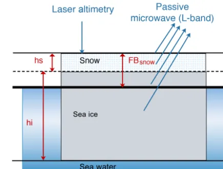
Basin-scale observation of the sea ice cover mainly relies on satellite-based remote sensing. Among the various sea ice parameters retrieved from satellite data, the most established is the sea ice concentration (or coverage). Figure 1 shows the various parameters related to satellite-based laser altime-try and (L-band) passive radiomealtime-try for the sea ice cover. Passive microwave remote sensing of both the Arctic and Antarctic is the basis of the retrieval of sea ice extent, with near-real-time coverage since about 1979 based on satellite campaigns such as Scanning Multichannel Microwave Ra-diometer (SMMR), the Special Sensor Microwave/Imager (SSM/I) (Cavalieri et al., 1999), AMSR-E (Comiso et al., 2003) and AMSR2 (Toudal Pedersen et al., 2017). However, the sea ice thickness is generally not retrievable through pas-sive remote sensing techniques due to the saturation of ra-diative properties especially for high-frequency ranges such as SMMR or SSM/I. In situ measurements of ice thickness through moored upward-looking sonar instruments and elec-tromagnetic induction sounders mounted on sledges, ships or helicopters/airplanes can provide sea ice thickness at specific locations or cross sections (Stroeve et al., 2014), so they are limited in terms of spatial coverage. Active remote sensing of satellite altimetry measures the overall height of the sea surface, serving as the major approach for the thickness re-trieval of the sea ice. For radar altimetry (RA), it is usually as-sumed that the radar signals penetrate the snow cover, and the main reflectance plane is the sea ice–snow interface (Laxon et al., 2003, 2013). Therefore in RA, the sea ice freeboard is measured. The sea ice thickness can be retrieved under cer-tain assumption of the snow loading, such as climatological snow depth data in Warren et al. (1999) for multi-year sea ice (MYI) and halved for the first-year sea ice (FYI). For laser altimetry as in ICESat (Kwok and Cunningham, 2008; Kwok et al., 2009), the main reflectance surface is the snow–air in-terface, and the directly retrieved value is actually the snow (or total) freeboard. The snow loading is also required for
Figure 1.Sea ice parameters in the active and passive remote sens-ing of the sea ice cover, includsens-ing sea ice thickness (hi), snow depth (hs) and snow freeboard (FBs).
the conversion of the snow freeboard to the sea ice thickness. As analyzed in Tilling et al. (2015) and Zygmuntowska et al. (2014), the uncertainty in snow depth is the most important contributor to that of the sea ice thickness and volume.
ous retrieval. It is found that the covariability of snow depth and freeboard at the local scale can greatly affect the well-posedness of the retrieval problem, and it is crucially impor-tant to include such covariability in the retrieval algorithm. Based on both realistic retrieval scenarios and large-scale re-trieval with OIB and SMOS data, we demonstrate that the proposed algorithm can simultaneously retrieve both sea ice thickness and snow depth, and the error in the retrieved pa-rameters mainly arises from the discrepancy between the sea ice area that corresponds to the SMOS measurement and that scanned by OIB. In Sect. 2 we first introduce the data, the models and the protocol of the combined retrieval. Detailed statistics of snow depth and the effects of covariability is cov-ered in Sect. 3. By integrating the covariability information, we propose the retrieval algorithm and carry out evaluation and analysis in Sect. 4. Section 5 summarizes the article and provides discussion of related topics and future work.
2 Data and models 2.1 Data
In order to construct and evaluate the retrieval algorithm, we mainly utilize two datasets, SMOS and OIB. SMOS measures the microwave radiation emitted from the Earth’s surface in L-band (1.4 GHz). In this article, we adopt the L3B TB product from SMOS. The daily gridded SMOS TB data field is generated from multiple snapshots within a day, with each snapshot involving multiple incident angles (rang-ing from 0 to 40◦) and spatially varying gain. The data are provided on the Equal-Area Scalable Earth (EASE) grid with a grid resolution of 12.5 km. However, due to the limitation of the satellite’s antenna size, the effective resolution of L-band radiometer onboard SMOS is about 40 km.
High-resolution airborne remote sensing of sea ice pa-rameters is available from OIB missions, starting in 2009 and covering the western Arctic during winter months (mainly around March). This paper utilizes OIB measure-ments from 2012 to 2015, during which the measuremeasure-ments include surface temperature of the sea ice cover. The prod-uct is organized into tracks and includes along-track
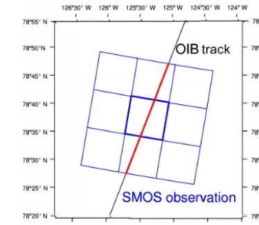
mea-Figure 2.Data match between OIB and SMOS data. SMOS TB product is provided on the 12.5 km EASE grid (shown by blue rect-angular cells). However, the inherent resolution of SMOS TB is of about 40 km. The red and black line represents the OIB track. Therefore, in order to accommodate the resolution differences, OIB samples that reside within the nine cells (red) are considered to be of equal contribution to the TB value at the central EASE grid cell (outlined by the thick blue line).
surements of total (or snow) freeboard, surface temperature and snow depth. Due to the nature of the airborne mea-surements, the observations are limited to a narrow swath on the order of 100 m. Snow freeboard products are pro-duced from Airborne Topographic Mapper (ATM) laser al-timeter (Studinger, 2010). Sea ice thickness is retrieved from snow freeboard (denoted FBs) and snow depth (denotedhs),
which is measured by the University of Kansas’ snow radar (Leuschen, 2014). Surface temperature is determined from the IceBridge KT-19 infrared radiation pyrometer dataset (Shetter et al., 2010). There is also accompanying sea ice type information, which is from EUMETSAT OSI-SAF sys-tem (Aaboe et al., 2016). Therein, the OIB Level-4 product IDCSI4 is adopted (Kurtz et al., 2013) for 2012–2013 and the remaining OIB data for 2014–2015 are from IDCSI2 Quick-look product, which is also available at NSIDC DAAC. Both of these datasets are 40 m in resolution in the along-track di-rection.
2.2 Data usage protocols
the daily gridded field is used in this study, we approximate the correspondence of OIB and SMOS TB by considering OIB measurements in the adjacent 3×3 cells (the red seg-ment in Fig. 2) of equal contribution to the SMOS TB at the central cell (the one bounded by thick blue lines in Fig. 2). In total, the nine cells cover an area of about 37.5 km×37.5 km, which is coherent with the physical resolution of SMOS data. It is worth noting that the area as covered by a single scan of the OIB track consists of less than 5 % of the total area that contributes to the SMOS TB. Therefore, we only treat the OIB data as samples of the underlying sea ice cover. The OIB sample count (denotedM) ranges from several hundreds to over 1000. The mean value ofM is about 700, but there exist certain areas that are scanned more extensively, which correspond to large values ofM. Figure A1 shows the distri-bution ofMfor all available OIB data.
In order to exclude the potential effect of insufficient sam-pling or the inhomogeneity of the sea ice cover, we further exclude the following data for the analysis and evaluation. First, if an area is under-sampled by OIB (M <100), it is not considered for further analysis. Second, we exclude the cases in which a single SMOS TB corresponds to OIB sam-ples with different sea ice types (i.e., mixed MYI and FYI). Third, we also exclude the cases involving sea ice leads as detected by the sea ice lead map in Willmes and Heinemann (2015a) or sea ice concentration lower than 1 according to Cavalieri et al. (1996). The purpose of these treatments is to rule out the factors that may compromise the quality of the OIB samples and allow focus on the discussion of the re-trieval algorithm.
The snow freeboard as measured by OIB and the SMOS TB is used as the input to the retrieval. The mean snow depth (hs) and mean sea ice thickness (hi) among OIB samples are
used for verification of the retrieval. Additionally, since we assume the underlying sea ice cover as homogeneous within the retrieval scale (within nine cells) and treat OIB measure-ments as samples to it, we also use theMmeasurements of snow depth to study the statistics of the snow depth and its covariability with snow freeboard.
2.3 L-band radiation model
The L-band (1.4 GHz) radiative property of the sea ice cover is characterized through numerical modeling based on Burke et al. (1979). The model was originally designed for the mod-eling of radiative transfer of the X- and L-band soil moisture. In Maaß et al. (2013b), this model is applied to sea ice and further used for the retrieval of snow depth over thick sea ice. In these works, a simple one-layer formulation is used for both the sea ice and the snow cover over it. In order to better characterize the radiative properties of the sea ice, in this article we use a multi-layer formulation of the model with sea ice type-dependent vertical salinity and tempera-ture profile (Zhou et al., 2017). The temperatempera-ture profile in the vertical direction is linear in either the snow cover or the
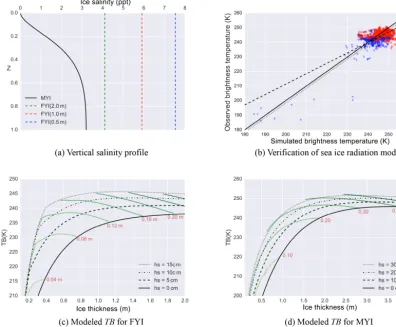
sea ice, assuming homogeneous thermal conductivity within the snow or the sea ice. Therefore the temperature in each sea ice or snow layer can be fully decided given the parame-ters of thermal conductivity, the ice bottom temperature (as-sumed to be−1.8◦C) and the snow surface temperature. The salinity profile of FYI differs from that of MYI. For FYI, the salinity of all layers of the sea ice all equals the bulk salin-ity, which decreases with the sea ice thickness. For MYI, a surface-drained profile is adopted to reflect the effect of sum-mer melt and flushing. Figure 3a shows the sea ice salinity profiles under the different sea ice types or thickness. The di-electric properties, the emissivity of the layers and the overall radiative properties of the sea ice cover are modeled, follow-ing Kaleschke et al. (2010) and Maaß et al. (2013b). The con-vergence of the modeled TB with respect to the layer count is witnessed, which is consistent with the study in Maaß et al. (2013b). In Zhou et al. (2017), it is demonstrated that the multi-layer treatment and the salinity profile MYI yield good fit between the simulated TB and SMOS TB. Appendix A covers details of the model and the verification with OIB and SMOS data. Figure 3c and d show the modeled TB under typ-ical sea ice parameters for FYI and MYI under typtyp-ical win-ter Arctic conditions (surface temperature of−30◦C). The green contour lines are constant FBs lines. With the
thick-ening of sea ice cover, the value of TB increases and satu-rates whenhiis large enough (larger than 2.5 m). The value
of TB is not monotonic with respect to FBs, and two
so-lutions are possible for certain value combinations of snow freeboard and TB. This results in the potential problem of ill-posedness of the retrieval with realistic observational data, as is discussed in Sect. 3.2.
Figure 3.L-band radiation model. Panel(a)shows sea ice salinity profile for FYI (dotted lines) and MYI (solid line). The vertical axis (z) is normalized with respect to the sea ice thickness. The comparison of the simulated TB based on OIB data and the observed SMOS TB is presented in panel(b). Blue triangles represent FYI, while red circles are MYI. The dashed (dotted) line is the least squares fit (least squares fit under the constraint that slope is 1). The root mean square error of TB is 3.1 K. Panels(c)and(d)show the modeled TB under typical sea ice parameters (hiandhs), assuming Arctic winter conditions (surface temperature of−30◦C). The green lines represent constant snow freeboard lines.
and the SMOS observation. Based on the aforementioned RMSE of 1.41 K for well-surveyed regions, we only consider the retrieval for cells with an TB error within 1.5 K for fur-ther studies. In all 412 TB cells are available, containing 35 OIB tracks and 321 168 OIB measurements. They account for about 50 % of all available TB cells. We consider this a limitation of combined usage of OIB and SMOS data, and the retrieval with actual satellite laser altimetry and L-band TB can be free from this limitation through better altimetric scanning and wider swath as compared with OIB.
2.4 Isostatic equilibrium model
Apart from the L-band radiation model, the other model as used by the retrieval is the equilibrium model based on the buoyancy relationship. Under certain assumptions of the sea ice density (denotedρice), seawater density (denotedρwater),
snow density (denotedρsnow) and the equilibrium state, the
sea ice thickness, snow depth and snow freeboard FBs are
constrained according to Eq. (1). The sea ice thickness can
be derived given the snow depth, according to Eq. (2). This model is widely applied for both radar and laser altimetry for the retrieval of sea ice thickness.
ρice·hi+ρsnow·hs=ρwater·(hi+hs−FBs) (1)
hi=
ρwater
ρwater−ρice ·FBs−
ρwater−ρsnow
ρwater−ρice
·hs (2)
In this study, ρwater and ρice are taken to be 1024 and
915 kg m−3, which are derived from field measurements dis-cussed by Wadhams et al. (1992), andρsnowis 320 kg m−3,
derived from Warren et al. (1999).
3 Retrievability analysis
Under the observational constraints of TB and FBs, both
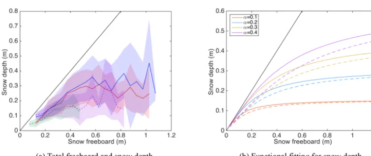
Figure 4.Statistics of snow depth from OIB at the local scale of retrieval. Panel(a)shows the mean and the±1 standard deviation of the snow depth within each snow freeboard bin (from 0 to 1.5 m by an interval of 5 cm), shown by lines and shaded areas for four realistic cases of OIB. Panel(b)shows the nonlinear fitting of snow depth over snow freeboard (Eq. 3) under representativesvalues (0.71 for FYI and 0.95 for MYI) and various values ofα. Solid color lines are for MYI and dashed ones for FYI. The solid black line isy=x.
snow freeboard lines (with freeboard values) are shown. With the observed TB and the corresponding observation of FBs,
the values of sea ice thickness and snow depth can be at-tained through a solving process that involves the two afore-mentioned forward models. The theoretical retrieval problem (shown in Fig. 3) is studied in Xu et al. (2017), with treatment of ill-posed cases which involve two potential solutions.
For the retrieval with actual observational data, the resolu-tion difference between the two types of observaresolu-tions should be accounted for. Previously in Sect. 2.2, we used a high-resolution altimetry scans as samples for L-band passive ra-diometry, which is of relatively coarser resolution. In this section we further analyze the statistical covariability be-tweenhsand FBson the scale of retrieval. Under the context
of retrieval, we base the analysis with the freeboard measure-ments as a priori and focus on how the snow depth changes with freeboard in a statistical sense. For each TB measure-ment, the multiple (M) OIB samples are subjected to statis-tical analysis, which shows that among these samples there exists statistically significant correlation between FBsandhs,
which can be better characterized by a nonlinear fitting. Fur-thermore, the effect of the covariability on retrievability is analyzed in Sect. 3.2.
3.1 Covariability analysis based on OIB data
For the covariability between FBsandhs, we choose the
na-tive resolution of the OIB product (40 m) as the spatial scale for analysis. Each TB corresponds to multiple (M) OIB sam-ples, with each sample containing the measurement for both FBsandhs. We divide these samples into FBsbins, with each
bin covering 5 cm. In total there are 30 bins, covering the range of 0 to 1.5 m. For samples in each bin, we compute the percentiles and the mean value of hs. Figure 4a shows
the meanhs and the±1 standard deviation range and their
relationship with FBs, for four representative TB points.
Fur-thermore, we carry out least squares linear fitting (weighted according to sample count in each bin) between FBs of the
bins and the corresponding meanhs in each bin. Among all
available data, there is statistically significant positive corre-lation betweenhs and FBs for over 90 % of all points. The
values ofR2 are in the range of 0.06 and 0.89 (95 % per-centile), with the mean value ofR2 as 0.53. This indicates that there is consistent covariability between snow depth and snow freeboard across Arctic sea ice cover.
However, for both FYI and MYI ice, there is saturation of the meanhs with respect to FBs. Besides, in the Arctic
in-undation is generally uncommon (i.e.,hs <FBs). In order
to accommodate these characteristics, we propose a nonlin-ear fitting, as shown by Eq. (3). The parametersαandβ are fitted according to observations. According to the equation, the value ofhs saturates toα·π/2 when FBs is large, and
the value ofα·β(denoteds), which is the slope of the func-tion at FBs=0, should be lower than 1 in order to avoid any
inundation.
hs(FBs)=α·arctan(β·FBs) (3)
Using Eq. 3, the overall quality of the fitting for all avail-able local OIB segments is improved, with mean value of
R2rising from 0.53 to 0.67, and the 95 % percentile of R2
Figure 5.Typical distributions of FBsand the range of meanhsfor 0< α <1. Panel(a)shows the four distributions (two for FYI and two for MYI) and the corresponding mean value of FBs. Global values ofsfor FYI and MYI are adopted. For these four distributions, panel(b) shows the meanhsfor the range ofαbetween 0 and 1. Meanhsincreases monotonically withαand saturates whenαis large.
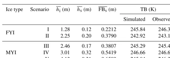
Table 1.Typical scenarios for retrievability studies. The mean sea ice thickness (hi), mean snow depth (hs), mean snow freeboard (FBs), observed TB from SMOS and the simulated TB from forward radiation model are shown. Scenarios I and II are FYI, and scenarios III, IV and V are MYI.
Ice type Scenario hi(m) hs(m) FBs(m) TB (K) Simulated Observed
FYI I 1.28 0.12 0.2212 245.84 246.38
II 2.25 0.20 0.3790 242.92 243.14
MYI
III 2.46 0.17 0.3807 245.29 245.46
IV 3.01 0.32 0.5419 246.66 246.61
V 4.13 0.31 0.6509 245.84 246.38
Furthermore, we consider the value ofsto be stable across either FYI or MYI sea ice and choose these values as univer-sal parameters for the design of the retrieval algorithm. Fig-ure 4b shows fitting function of snow depth over snow free-board based on these representative values ofsunder various values forα.
3.2 Effects of covariability on retrievability
We evaluate the covariability and its effect on retrieval from several aspects. We choose five realistic retrieval scenarios among all the OIB and SMOS data, with two of them repre-senting FYI retrieval and three of them for MYI. As shown in Table 1, they represent typical retrieval problems for Arc-tic sea ice. Besides, the simulated TB values by the radi-ation model is close to the corresponding SMOS TB val-ues (within 1.5 K). Based on these scenarios, we examine whether it is possible to retrieve the actual sea ice thickness and snow depth, with or without the covariability. Firstly we ignore the covariability and assume a flat snow cover: for the
MOIB samples, we assume that the snow depth is uniform. For the retrieval problem, since the directly observed values are freeboard samples (FBs|m, where mis the index of the
samples, and 1≤ m≤ M), we carry out the scanning of the (uniform) snow depthhsfrom 0 m (snow free) to 1 m
(suffi-ciently deep). Under a certain value ofhs, we retrieve the sea
ice thicknesshi|mfor each FBs|mwith Eq. (2), based on the
current value ofhs. Then the TB value for this sample (TB|m)
can be calculated according to the L-band radiation model, withhi|m,hsand surface temperatureTsfc|m. The mean TB
value is then computed as the arithmetic mean of all TB|m’s, for the current value ofhs. For any OIB sample, if the value
of freeboard is smaller than the current value ofhs, in order to
avoid inundation, the snow depth for this sample is assumed to be the same as FBs. If the number of samples that witness
potential of inundation over 50 % ofM, we stop the scanning even ifhshas not reached 1 m.
In order to incorporate the effect of covariability, we adopt either the global value ofs(0.71 for FYI and 0.95 for MYI) or the locally fitted value ofs(specific to each scenario) and carry out the retrieval. Figure 5a shows four typical distri-bution of FBs, and Fig. 5b shows a range of values forα(0
to 1) and the resulting mean value ofhsfor the four typical
distributions. For the range of 0 to 1, the resulting meanhs
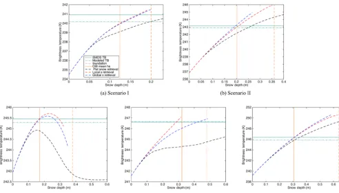
Figure 6.Retrievability study with different retrieval scenarios. The horizontal solid (dotted-dashed) lines are the SMOS (modeled) TB. The vertical solid lines represent the values of the mean snow depth from OIB observation. The black dashed curves denote the values of TB generated by scanning ofhsunder the flat snow cover assumption, and the vertical dashed lines denote the values ofhsthat result in 50 % OIB samples to be inundated. The red (blue) dashed curves (with the corresponding mean snow depth) are the values of TB generated by scanning ofαwith the local (global) values ofsas in Eq. (3).
small for whole range FBs, resulting in a very small value
of meanhs. Furthermore, the value of meanhsapproaches 0
when αapproaches 0, which in effect corresponds to “bare ice”. With the grow ofα, there is a monotonous increase in the mean hs; and whenαis large enough, the meanhs
sat-urates. For all four FBs distributions, we consider that the
resulting mean hs is reasonable for the range of α.
There-fore, the retrieval of snow depth is attained by locating the proper value ofα. Due to the potential of double solution in the retrieval, the solving ofαis attained by a scanning pro-cess that covers the reasonable range forα. The scan starts from 0.001 and steps by 0.01, and it is limited to a large value that yields saturation for meanhs. With each scanned value
ofα, a corresponding value forβ, can be computed ass / α, and the snow depthhs|m for each sample can be computed
with Eq. (3). Then thehi|m, the TB values for each sample
can be computed, as well as the mean snow depth and mean TB.
We record the (mean) snow depth and the corresponding mean TB across the scanning process. Figure 6 shows the results of scanning for the five scenarios in Table 1. Note that for the lines that represent scanning of α(i.e., involv-ing covariability), thex axis is the resulting values of mean
hs, notα. The observed TB and the simulated TB (with OIB
data) are shown by solid and dot-dashed horizontal lines, re-spectively. Besides, the observed mean snow depth and the 50 % inundation with flat snow cover are shown by solid and dashed vertical lines, respectively. The simulated TB with flat snow cover (black dashed curve in each subfigure) is always lower than that with covariability information (blue dashed curves for results with globals and red ones for those with locals). For all the scenarios, the TB values that are attained through scanning can reach the observed TB with the incor-poration of covariability, while the values of TB in two sce-narios (III and IV) fail to reach the observation with the flat snow cover assumption. This implies that with the flat snow cover assumption, there is no solution to the retrieval prob-lem. We further examine the other three scenarios; the so-lutions of the retrieval problem reside at the cross point of the scanned TB curves and the horizontal bars that represent observational TB values. The solutions of mean snow depth under the flat snow cover assumption are always larger than the observed mean snow depth by over 5 cm.
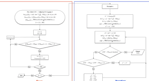
Figure 7.Flow chart for retrieval algorithm. Two phases are marked out. The red box includes the scanning process for the potential solutions to the retrieval problem, and the blue box shows the iterative binary search for the solving process.
observed snow depth. The differences between the solutions produced by scanning and the observed snow depth are 5 cm or larger for scenarios I and V, while the scanning with local
s produces smaller errors. It is worth noting that for the ac-tual retrieval process, the local value ofsis not available, and only the global value ofsis usable. Lastly, for scenario III, two potential solutions exist (two crossing points between the TB scanning curve and the observational TB). Without extra observational data during retrieval, it is not possible to judge which solution is the true (or better) one. Therefore the retrieval algorithm should be able to locate both possible solutions.
The covariability as observed with OIB data plays an im-portant role in the retrievability of the sea ice parameters. Also with OIB data, we extract the statistical relationship (Eq. 3) that characterizes the covariability which can be in-corporated in the retrieval. However, during retrieval, the pa-rameter s is generally not available for the local area, and the global values ofs(for FYI and MYI) as computed from high-resolution OIB data can be adopted.
4 Retrieval algorithm and evaluation
With the statistically significant covariability, we design the retrieval algorithm for sea ice thickness and snow depth that includes two distinctive phases. The overall structure of the algorithm is similar to the theoretical retrieval algorithm in
Xu et al. (2017). The incorporation of covariability is further integrated, based on the nonlinear fitting in Eq. (3) and the fixed value ofs for both FYI and MYI derived from OIB data. The first phase involves the scanning of possible snow depth configurations. This phase is in effect carried out by the scanning of the value ofαfrom 0.001 to 3 (or sufficiently large). A possible solution is detected between two adjacent values ofα, when the TB values as generated with these two values ofαare on different sides of the observed TB. During the second phase, all the possible solutions are then attained with an iterative binary search ofα. All possible solutions are reported by the retrieval algorithm. The outline of the al-gorithm is presented in Fig. 7, with the two phases marked out by red and blue boxes, respectively. We also construct a reference retrieval algorithm based on the flat snow cover assumption, for which the scanning is over the snow depth instead ofα. The details of this reference algorithm is omit-ted for brevity.
For the typical scenarios in Table 1, we carry out the re-trieval for the mean sea ice thickness (hi) and the mean snow
depth (hs) using the standard algorithm with either the global
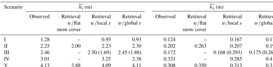
or the local values ofs, as well as the reference algorithm. Table 2 shows the comparison of the retrieval results and observations. The reference algorithm (with flat snow cover assumption) consistently performed worse than the standard algorithm. For scenarios I and IV, it failed to attain any solu-tion. For the standard algorithm, small error in bothhiandhs
Table 2.Retrieved results (hiandhs, in units of meters) for five scenarios under different retrieval algorithms. In scenarios II, IV and V, the retrieval with flat snow cover assumption is unsuccessful. The values in the brackets for scenario V denote the other (possible) solution for sea ice parameters.
Scenario hi(m) hs(m)
Observed Retrieval Retrieval Retrieval Observed Retrieval Retrieval Retrieval
w/flat w/locals w/globals w/flat w/locals w/globals
snow cover snow cover
I 1.28 – 0.95 0.93 0.124 – 0.167 0.171
II 2.25 2.00 2.23 2.30 0.202 0.263 0.207 0.195
III 2.46 – 2.50 (1.69) 2.45 (1.88) 0.172 – 0.168 (0.293) 0.175 (0.263)
IV 3.01 – 3.25 2.38 0.321 – 0.285 0.419
V 4.13 3.88 4.09 4.11 0.308 0.350 0.313 0.310
as compared the retrieval with the global values ofs. Besides, for scenario III for which two solutions are possible, the re-trieval algorithm addresses both of them. The rere-trieval results are consistent with the retrievability analysis in Sect. 3.2.
We further carry out verification of the retrieval algorithm in two aspects. First, by using all available OIB data, we simulate the retrieval problem with laser altimetry measure-ments and verify the retrievedhi andhs against OIB
mea-surements. Section 4.1 covers the retrieval and analysis. Fur-thermore, we construct several representative retrieval sce-narios in Sect. 4.2 and analyze the uncertainty in the retrieved parameters and carry out attribution of the uncertainty to in-put parameters of the retrieval.
4.1 Large-scale retrieval
For the systematic verification of the proposed algorithm, we carry out the retrieval with all the available OIB data (as mentioned in Sect. 2.3) from 35 OIB tracks and 412 SMOS TB measurements, which correspond to 412 retrieval cases. For each SMOS TB, the corresponding samples (snow freeboard, surface temperature and sea ice type) from OIB dataset are used as the input for the retrieval. The retrieval with the flat snow cover assumption (the reference algorithm) is only successful for 50 cases, which accounts for about 12 % of available cases. For comparison, the (standard) algo-rithm achieves retrieval for 391 cases (95 %) with the global
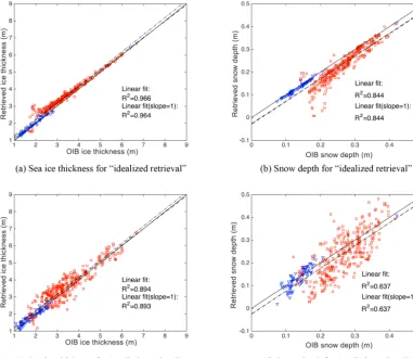
s values and for all the TB values with the locally fits val-ues. Figure 8 shows the comparison of retrieved mean sea ice thickness and snow depth with observations. Figure 8a and b shows the results forhiandhs, based on (1) simulated
TB (as computed from the radiation model) and (2) the local value ofs. This represent the “idealized” retrieval problem in which there exists no extra uncertainty. As shown in Fig. 8a, the LSQ fit for hi (dash line) features aR2value of 0.966,
while the LSQ fit under the extra constraint on slope (dot-ted dash line) features aR2value of 0.964. For snow depth (Fig. 8b), the R2values for the two fittings are both 0.844.
This indicates that the retrieval is in good agreement with the observations.
For the actual retrieval problem for which the local value of s is unknown, and the observational TB values from SMOS are used, Fig. 8c and d show the evaluation for hi
andhs, respectively. The fitting quality (in terms ofR2) for
sea ice thickness is as high as 0.89 and that for snow depth is 0.637. It is worth noting that these results are achieved with only statistical data derived from large-scale OIB sur-veys. Furthermore, if the retrieval is based on (1) observed TB from SMOS and (2) the locally fitted value of s, the
R2values for the fitting are 0.91 and 0.65 for sea ice thick-ness and snow depth, respectively, with virtually no change in the fitting lines (not shown). There is minor increase in quality (0.91 versus 0.89 and 0.65 versus 0.637) and a rela-tively large gap to the “idealized” retrieval. As a comparison, we also carry out retrieval with the TB with forward model and the local values ofs, and theR2for fittings between the retrieved and the observed parameters for sea ice thickness and snow depth are 0.96 and 0.84, respectively. This indi-cates that the difference (or error) of the modeled and the ob-served TB plays an important role in affecting the quality of the retrieval. The discrepancy between the observed TB and the modeled TB may arise from (1) the imperfect radiation model, including its formulation as well as the model param-eters, or (2) the mismatch between the altimetry scans and L-band passive observations, as introduced in Sect. 2.2. The areas with more extensive OIB scans are shown of lower TB error (see Fig. A2), indicating that the error in the retrieved parameters can be potentially reduced with better altimetry coverage.
For comparison, we also carry out the retrieval which only involves TB and the mean value of FBs. This retrieval
problem ignores the resolution difference between altimetry scans and L-band radiometry and generally corresponds to the theoretical retrieval problem analyzed in Xu et al. (2017). Specifically, for the use of OIB data, the mean value ofM
samples of FBs is computed and further combined with TB
Figure 8.Large-scale retrieval of mean sea ice thickness(a, c)and mean snow depth(b, d)and verification with OIB observations. In each panel, blue triangles (red rectangles) denote FYI (MYI), the solid line is the 1:1 line and the dashed (dashed dotted) line represents the linear fitting (linear fitting line with the constraint that the slope be 1). The quality of fittings in terms ofR2are also shown. Panels(a, b) represent the comparison results for the retrieval with modeled TB and the local values ofs. Panels(c, d)represent the results with SMOS TB and the global values ofsas derived from OIB data.
only the mean FBs is involved in the retrieval, covariability
does not play a role in the retrieval. By using the same SMOS and OIB data as the evaluation in Fig. 8, the retrieval yields
R2 of 0.78 and 0.50 for hi and hs (fitting between the
re-trieved and the observed parameter). For comparison, under the realistic retrieval results (Fig. 8c and d), the quality of re-trieval is much improved for bothhi(R2from 0.78 to 0.89)
and hs (R2 from 0.50 to 0.64). This demonstrates that the
high-resolution altimetry samples and the accompanying co-variability information play an important role in improving the quality of the retrieval.
Based on the retrieval with large-scale observational data, the proposed algorithm achieves effective retrieval of both sea ice thickness and snow depth, by using simultaneous re-mote sensing of the sea ice cover, i.e., laser altimetry and L-band passive microwave sensing. The statistics of snow depth and its covariability with snow freeboard on the spa-tial scale of retrieval play an important role in improving the
well-posedness of the retrieval problem as well as the quality of the retrieved parameters.
4.2 Uncertainty analysis
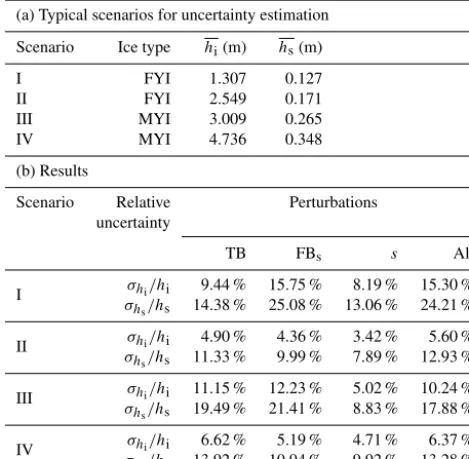
In order to assess the uncertainty of the retrieved parame-ters, we further design four realistic retrieval scenarios from OIB and SMOS data listed in Table 3a. Due to the nonlinear relationship between sea ice parameters and TB, we cannot directly compute the uncertainty inhiorhs. Instead, Monte
Carlo (MC) simulation is adopted. For each scenario in Ta-ble 3a, four sets of MC simulations are constructed, each containing: (1) random perturbations to TB only, (2) random perturbations to FBsonly, (3) random perturbations tosonly,
and (4) random perturbations to TB, FBs ands altogether.
Each set contains 1000 random sampling to these parame-ters.
uncer-Table 3.Uncertainty estimation for typical retrieval scenarios.
(a) Typical scenarios for uncertainty estimation
Scenario Ice type hi(m) hs(m)
I FYI 1.307 0.127
II FYI 2.549 0.171
III MYI 3.009 0.265
IV MYI 4.736 0.348
(b) Results
Scenario Relative Perturbations uncertainty
TB FBs s All
I σhi/hi 9.44 % 15.75 % 8.19 % 15.30 % σhs/hs 14.38 % 25.08 % 13.06 % 24.21 %
II σhi/hi 4.90 % 4.36 % 3.42 % 5.60 % σhs/hs 11.33 % 9.99 % 7.89 % 12.93 %
III σhi/hi 11.15 % 12.23 % 5.02 % 10.24 % σhs/hs 19.49 % 21.41 % 8.83 % 17.88 %
IV σhi/hi 6.62 % 5.19 % 4.71 % 6.37 % σhs/hs 13.92 % 10.94 % 9.92 % 13.28 %
tainty). The perturbations to theM values of FBs are based
on OIB data specification and follow log-normal distribution. The perturbations to s are specific to sea ice type (FYI or MYI) and based on the statistics of s as derived from all OIB data. As shown in Appendix B, the distribution of s
can be well characterized by beta distribution for both FYI and MYI. The fitting to beta distribution is then carried out for both FYI and MYI according to Eq. (4), wherea,band const are fitted parameters by using OIB data at 40 m resolu-tion (see Fig. B3). For FYI,a,band const are 4.31, 2.00 and 1.00, respectively, and for MYI are 4.25, 2.06 and 1.2.
f (x|a, b,constant)= const
B(a, b)x
(a−1)(1−x)(b−1) (4)
The perturbations to sfollow the fitted beta distribution. Furthermore, the perturbations to TB, FBs andsare treated
as independent. Each MC simulation (of 1000 simulations) contains a set of perturbed input parameters and corresponds to a retrieval problem. Based on the results from the 1000 simulations, the uncertainty of the retrieved hi and hs are
computed by biased standard deviation estimation with re-spect to the original retrieval which involves no perturbation. Table 3b shows the relative uncertainty ofhiandhsfor each
experiments for all scenarios. First, the relative uncertainty for hiorhs is at most about 25 %. Also, all scenarios show
thatsplays a minor role in terms of uncertainty, as compared with TB or FBs. TB and FBs play a comparable role in the
uncertainty of the retrieved parameters. Moreover, for both FYI and MYI, the uncertainty in the retrieved hi andhs is
relatively lower for thicker ice and deeper snow cover. The uncertainty of TB (or FBs) is not correlated spatially and that
of sis based on basin-scale statistics from OIB. Therefore,
the uncertainty of the retrievedhi(orhs) is not spatially
cor-related, resulting in effective reduction of the uncertainty in the sea ice volume (or snow volume).
5 Summary and discussion
In this study, we introduce a new algorithm for retrieving multiple Arctic sea ice parameters based on a combination of L-band passive microwave remote sensing and active laser altimetry. Two physical models, the L-band radiation model and the buoyancy relationship, are adopted to constrain the sea ice thickness and snow depth. They are used as forward models during an iterative retrieval process that solves the sea ice parameters that satisfy the observed L-band TB and snow freeboard values. Specifically, according to high-resolution observations, there is statistically significant covariability be-tween the snow depth and the snow freeboard. This informa-tion of covariability is further incorporated in the retrieval algorithm, and it is demonstrated that the covariability plays a key role in the retrievability. Specifically, a nonlinear fit-ting that characterizes the covariability is derived from OIB data, and a parameter (initial slope of the fitting function) is considered invariant for FYI and MYI and further adopted by the retrieval algorithm. Verification with available OIB data shows that both sea ice thickness and snow depth are retrieved, with the error in both parameters mainly arising from the mismatch between modeled and observed TB val-ues. This algorithm can be applied to the large-scale retrieval of sea ice thickness and snow depth using concurrent L-band satellite remote sensing and satellite altimetry of the sea ice cover such as Abdalati et al. (2010).
5.1 Difference with existing retrieval algorithms
the analysis in Kwok et al. (2011) is carried out on coarser spatial scales, our work focuses on the spatial scale that is rel-evant to the retrieval of sea ice parameters. We demonstrate that on this relatively small spatial scale, there still exists co-variability between snow depth and snow freeboard. 5.3 Uncertainty estimation related to model
parameters
Besides the input parameters to the retrieval (TB, FBsands),
model parameters also play an important role in modulating the uncertainty for retrieval (Zygmuntowska et al., 2014; Xu et al., 2017). For this study, we adopt constant parameters for density values following protocols of OIB, mainly for the di-rect comparison with OIB dataset. However, their effect on the uncertainty of retrieved parameters should be accounted for in a systematic approach, similar to Xu et al. (2017). MC simulations can be adopted for the quantification of the un-certainty through perturbations to both input and model pa-rameters.
5.4 Outlook of satellite-based retrieval
The proposed retrieval method is the basis for the retrieval of sea ice parameters with data from concurrent satellite cam-paigns. Although there was no concurrent L-band satellite observation with the ICESat campaign, there are candidate satellite campaigns such as WCOM (Shi et al., 2016), which provides concurrent L-band observation with the planned ICESat-2 campaign. For the study with satellite data, there are several practical issues. First, the snow surface tempera-ture is provided by airborne sensors in OIB but is not gener-ally available with laser altimetry. Several data sources serve as candidate data for the concurrent surface temperature field, such as reanalysis data (Dee et al., 2011), a MODIS-based product (Hall et al., 2004). Second, there is small-scale variability of the sea ice cover such as leads, which were not considered for the analysis and verification in this study. As shown in Zhou et al. (2017), the presence of sea ice leads has a profound effect in lowering the overall TB on the scale of SMOS observations. Leads can be treated as small-scale heterogeneity of the sea ice cover, and the incorporation of
cific resolution of the satellite altimetry. By using 70 m as the typical resolution of ICESat-2, we deduce the value of
sat this resolution by manual coarsening OIB’s data by av-eraging adjacent points. In effect, the value ofs at 80 m is computed, which shows a slight decrease ofs for both FYI and MYI. Figure B3 shows the general scaling ofsfor the resolution range from 40 to 240 m. Fourth, in order to esti-mate the uncertainty of the retrieved parameters, the effects of surface temperature, as well as other data sources (includ-ing TB, freeboard measurements and the value ofs), should be evaluated in a systematic way. Due to the nonlinear re-lationship between TB and the sea ice parameters, MC sim-ulations can be carried out for the quantification of the un-certainty. Besides, for the historical data from ICESat (Kwok and Cunningham, 2008) during the first decade of the 21st century, due to the lack of basin-scale L-band observation for the Arctic, other passive remote sensing data such as C-band data from AMSR-E can be exploited in a similar manner for the retrieval of these historical data.
The native spatial resolution of AMSR-E based C-band remote sensing product is over 60 km, which is coarser than that of SMOS L-band data but provides similar, daily cov-erage for the Arctic. Therefore, the resolution difference be-tween AMSR-E based C-band data products and ICESat data should be accounted for in a similar approach as in Sect. 2.2. Besides, due to the relatively shorter wavelength of C-band as compared with L-band, the penetration depth of C-band signal in sea ice cover is potentially shallower, resulting in more premature saturation of C-band signal to sea ice thick-ness. Under the assumption of a uniform and dry snow cover, the relatively long wavelength of C-band and L-band ensures that the snow cover is “transparent” to the L- or C-band sig-nal. For L-band and C-band, there is good potential for re-trieval through the thermodynamical modulation of the sea ice thickness by the snow cover, as indicated by Maaß et al. (2013a).
passive campaigns, including SMOS, SMAP and AMSR2. According to the theoretical study by Xu et al. (2017), the retrieval that combines RA with L-band data is potentially free of the ambiguous solutions present in this study. Be-sides, there also exists resolution differences between RA (e.g., 300 m for CryoSat-2) and L-band data such as SMOS. Measurements from RA can be treated as high-resolution sampling of the sea ice area that corresponds to a single L-band TB. Furthermore, based on the analysis and methods proposed in this article, the covariability between snow depth and sea ice freeboard can be further incorporated in the com-bined retrieval with RA and L-band passive remote sensing data.
Data availability. SMOS data are provided by the Integrated
The modeling of the radiative properties of the sea ice cover includes four types of media in the vertical direction: seawa-ter beneath the sea ice, sea ice, snow cover over the sea ice and air. The seawater (air) is considered to be semi-infinite beneath (above) the sea ice cover. The sea ice is further di-vided intoN layers in the vertical direction, with each layer of the same height. For the snow cover, a homogeneous struc-ture is assumed, with prescribed parameters such as thermal conductivity and permittivity. Also, a dry snow cover is as-sumed, and snow morphology features (such as differentia-tion between wind slab and depth hoar) and other vertical structures are not considered. The (SMOS) observed bright-ness temperature (TB) is assumed to be the multi-angle mean (0–40◦) TB as radiated from the aforementioned multi-layer media.
A2 Temperature and salinity structure
The radiation model characterizes the vertical structure of the sea ice cover by specifying the temperature and salinity of each layer based on the sea ice type and the snow surface temperature (Tsurf). The vertical temperature profile is
deter-mined by the overall thermal condition as defined by Tsurf
and the thermal conductivity for sea ice (kice) and that of
snow (ksnow). The bottom of the sea ice is assumed to be at
freezing temperature of−1.8◦C (denotedTwater). Based on
observation-based fittings in Untersteiner (1964) and Yu and Rothrock (1996),kiceandksnoware defined as follows.
kice=2.034 W m−1K−1+0.13 W kg−1m−2
Sice
Tice−273.15
ksnow=0.31 W m−1K−1
In this study, we consider the change of kice within the
sea ice of minor effects and use a bulk value for kice,
re-sulting in a linear temperature profile within the sea ice. This bulk value is determined by the bulk value ofSice. The
temperature profile is assumed to be continuous through the media interfaces, and ice temperature is assumed to equal the snow temperature at the snow–ice interface. GivenTsurf
based on other observations (such as MODIS), the bulk ice
Figure A1.Distribution of OIB sample count (M).
and snow temperaturesTiceandTsnowcan be written as
fol-lows (K=(ksnowhi+kicehs)−1).
Tice=Twater+
1
2K (Tsurf−Twater) ksnowhi
Tsnow=
1
2(Twater+Tsurf+K (Tsurf−Twater) kicehs)
Since a bulk value is adopted for bothkiceandksnow, given
any Tsurf, the temperature profile is linear within the snow
cover, as well as the sea ice. Then, the temperature of each layer of the sea ice cover can be computed.
For the salinity, sea ice type is considered with differentia-tion between MYI and FYI. For FYI, the salinity is assumed to be homogeneous in the vertical direction and equals the bulk salinity as prescribed by the sea ice thickness. The bulk salinity for FYI is in turn adapted from the multi-linear struc-ture in Cox and Weeks (1974) and defined as follows (where the ice salinity, denotedSice, is in ppt).
Sice=6.08·e(−5.81·hi)+7.409·e(−0.5228·hi)
With the deepening of the FYI sea ice cover, the bulk salin-ity decreases, and its minimum value is kept above 1.5 ppt. In contrast, for MYI, in order to reflect the effect of brine drainage and flushing during the melt season, a vertical salin-ity profile is adopted following Schwarzacher (1959). For the
kth sea ice layer (k=0 for the surface layer of the sea ice), the mean salinity (Si,k) is prescribed as
Si,k=
1 2Smax
h
1−cosπ za/(z+b)i.
A normalized vertical coordinate (z) is adopted with re-spect to sea ice thickness, starting from z=0 for the ice surface to z=1 for the bottom of the ice. For layer k,
z=(k−1/2)/N and the corresponding salinity of the layer can be computed. N is the total number of ice layers, and
Smax=3.2 ppt,a=0.407 andb=0.573, which are the fitted
parameters from in situ observations of MYI salinity. There-fore, for MYI, the sea ice salinity ranges from 0 at the top of the surface (z=0) toSmaxat the bottom (z=1). The
Figure A2.The relationship of RMSE of TB to OIB sample count (M). The statistics of RMSE of TB are computed for each sample count bin (each of 100). Shaded area covers the 5th and 95th per-centile of the absolute TB error.
A3 Radiative properties
The radiation model describes the radiation emitted from snow cover, sea ice and seawater; the brightness temperature at the top of atmospheric (TBTOA) can be described as (Maaß
et al., 2013b)
TBTOA=(1−c)·(TBwater+(1−ewater)·TBcosm)
+c·(TBice+(1−eice)·TBcosm)+1TBatm. (A1)
In Eq. (A1),cis sea ice concentration,eice and TBice are
the emissivity and TB of sea ice,ewaterand TBwater are the
emissivity and TB of seawater, and TBcosm is cosmic
mi-crowave background radiation, which can be considered as uniform and constant (2.7 K). 1TBatm is TB from
atmo-spheric contribution ranging from−0.36 to+5.67 K. Emis-sivity parameters are computed as follows:ewateris based on
the Fresnel equations in different directions of polarization (Ulaby et al., 1986) andeiceis a function of parameters such
as polarization, incidence angle, sea ice thickness, temper-ature, density, salinity, surface roughness, snow depth and temperature. Based on Maaß et al. (2013b), the permittivity of snow (snow) is determined by a polynomial fit obtained
from measurements at microwave frequencies ranging be-tween 840 MHz and 12.6 GHz (Tiuri et al., 1984) as follows.
snow=
1+0.7ρsnow+0.7ρsnow2
+i·
1.59×106×
0.52ρsnow+0.62ρsnow2
·
f−1+1.23×10⁻¹⁴pfe0.036T,
whereρsnowis the relative density of snow (compared to
wa-ter),T the temperature of snow in degrees Celsius andf the microwave frequency. It should be noted thatsnowdepends
on the snow wetness, which is not considered by the current model. Permittivity of sea ice (ice) is confirmed by brine
vol-ume fraction (Vb) using empirical relationship in Vant et al.
(1978).
ice=a1+a2Vb+i·(a3+a4Vb)
Vbis given in ‰, and the values ofa1,a2,a3anda4follow
Kaleschke et al. (2010). Similar to Maaß et al. (2013b), for the permittivity of seawater (water), the empirical
relation-ship from Klein and Swift (1977) is adopted, and the permit-tivity of air (air) is assumed to be 1. The brine volume
frac-tionVbcan be expressed in the following (Cox and Weeks,
1983).
Vb=
ρiceSice
ρbrineSbrine(1+k)
Sice is the ice salinity, ρice the ice density, Sbrine the brine
salinity andρbrine the brine density.ρbrine can be fitted with
Sbrine(in ‰) according to Cox and Weeks (1983).
ρbrine=1+0.0008·Sbrine
Then the following equation is adopted to relateSbrinewith
Tice(Vant et al., 1978):
Sbrine=a+b·Tice+c·Tice2 +d·Tice3,
whereTiceis in◦C anda,b,candd are fitted parameters in
Vant et al. (1978). These polynomial approximations agreed well with the experimental data in Zubov (1963). Also,ρice
can be expressed by ice temperature (Tice: ◦C) in Pounder
(1966):
ρice=0.917−1.403×10⁻⁴Tice
Therefore,Vbcan be expressed as a function ofρice,Sice
andTice.
As derived model from Burke et al. (1979), the radiation model is a coherent model. However, the effect of non-coherency is considered to be mitigated by several factors. First, with the SMOS observations, there is large variability of both sea ice thickness and snow depth within the typical resolution of 40 km. There usually exists large variability of the sea ice cover within the spatial scale of 40 km (variabil-ity ofhi larger than one-quarter of the L-band wavelength),
which effectively mitigates the effect of non-coherency, as indicated in Kaleschke et al. (2010). Furthermore, multi-angle mean of SMOS TB further introduces a range of in-tegration path of radiations. The multi-layer treatment of the sea ice is also explored in Maaß et al. (2013b). According to the study in Zhou et al. (2017), with treatment of the salinity profile in MYI (i.e., salinity drainage in the top layers), the modeled TB is more consistent with the SMOS TB.
Under typical winter Arctic conditions (Tsurf=−30◦C),
eled vs. observed by SMOS) is 3.1 K for all available OIB data (see also Fig. 3c). If we further limit the computation of RMSE to the points with large values ofM(95th percentile forM, corresponding to areas with good OIB coverage), the RMSE drops to 1.41 K. Figure A2 shows the relationship of TB error and M. As shown, there is a drop in both RMSE and the maximum error of TB with better spatial coverage of OIB. The lead information can be further incorporated in the radiation model (Zhou et al., 2017), which effectively re-duces the overestimation of TB as caused by refrozen leads or open water.
Figure B1.Distribution ofα,βandsfor FYI. Data of 40 m resolution (OIB) are used for computing the value of each parameter on the scale of 37.5 km (i.e., approximately the native resolution of SMOS TB).
Figure B2.Same as Fig. B1 but for MYI.
Reviewed by: four anonymous referees
References
Aaboe, S., Breivik, L.-A., Eastwood, S., and Sorensen, A.: Sea Ice Edge and Type Products, http://osisaf.met.no/p/ice/edge_type_ long_description.html, last access: 30 December 2016.
Abdalati, B., Zwally, H., Bindschadler, R., Csatho, B., Farrell, S., Fricker, H., Harding, D., Kwok, R., Lefsky, M., Markus, T., Mar-shak, A., Neumann, T., Palm, S., Schutz, B., Smith, B., Spin-hirne, J., and Webb, C.: The ICESat-2 laser altimetry mission, in: Proceedings of the IEEE, 98, 735–751, 2010.
Brucker, L. and Markus, T.: Arctic-scale assessment of satellite pas-sive microwave-derived snow depth on sea ice using Operation IceBridge airborne data, J. Geophys. Res.-Oceans, 118, 2892– 2905, 2013.
Burke, W. J., Schmugge, T., and Paris, J. F.: Comparison of 2.8- and 21-cm microwave radiometer observations over soils with emis-sion model calculations, J. Geophys. Res., 84, 287–294, 1979. Cavalieri, D., Parkinson, C., Gloersen, P., and Zwally, H.: Sea
Ice Concentrations from Nimbus-7 SMMR and DMSP SSM/I-SSMIS Passive Microwave Data, Boulder, Colorado USA. NASA National Snow and Ice Data Center Distributed Ac-tive Archive Center, https://doi.org/10.5067/8GQ8LZQVL0VL, 1996.
Cavalieri, D. J., Parkinson, C. L., Gloersen, P., Comiso, J. C., and Zwally, H. J.: Deriving long-term time series of sea ice cover from satellite passive-microwave multisensor data sets, J. Geo-phys. Res., 104, 15803–15814, 1999.
Comiso, J., Cavalieri, D., and Markus, T.: Sea ice concentration, ice temperature, and snow depth using AMSR-E data, IEEE T. Geosci. Remote, 41, 243–252, 2003.
Comiso, J. C., Parkinson, C. L., Gersten, R., and Stock, L.: Acceler-ated decline in the Arctic sea ice cover, Geophys. Res. Lett., 35, L01703, https://doi.org/10.1029/2007GL031972, 2008. Cox, G. F. and Weeks, W. F.: Salinity variations in sea ice, J. Glaciol,
13, 109–120, 1974.
Cox, G. F. and Weeks, W. F.: Equations for determining the gas and brine volumes in sea-ice samples, J. Glaciology, 29, 306–316, 1983.
Dee, D., Uppalaa, S., Simmonsa, A., Berrisforda, P., Polia, P., Kobayashib, S., Andraec, U., Balmasedaa, M., Balsamoa, G., Bauera, P., Bechtolda, P., Beljaarsa, A., van de Berg, L., Bidlota, J., Bormanna, N., Delsola, C., Dragania, R., Fuentesa, M., Geera,
https://doi.org/10.5194/tc-4-583-2010, 2010.
Klein, L. and Swift, C.: An improved model for the dielectric con-stant of sea water at microwave frequencies, IEEE T. Antenn. Propag., 25, 104–111, 1977.
Kurtz, N., Markus, T., Farrell, S., Worthen, D., and Boisvert, L.: Observations of recent Arctic sea ice volume loss and its impact on ocean-atmosphere energy exchange and ice production, J. Geophys. Res., 116, C04015, https://doi.org/10.1029/2010JC006235, 2011.
Kurtz, N. T. and Farrell, S. L.: Large-scale surveys of snow depth on Arctic sea ice from Operation IceBridge, Geophys. Res. Lett., 38, L20505, https://doi.org/10.1029/2011GL049216, 2011. Kurtz, N., Studinger, M., Harbeck, J., Onana, V., and Farrell, S.: .
IceBridge Sea Ice Freeboard, Snow Depth, and Thickness, Ver-sion 1. [Indicate subset used], Boulder, Colorado USA, NASA National Snow and Ice Data Center Distributed Active Archive Center, https://doi.org/10.5067/7XJ9HRV50O57, 2012 (updated 2015).
Kurtz, N. T., Farrell, S. L., Studinger, M., Galin, N., Harbeck, J. P., Lindsay, R., Onana, V. D., Panzer, B., and Sonntag, J. G.: Sea ice thickness, freeboard, and snow depth products from Oper-ation IceBridge airborne data, The Cryosphere, 7, 1035–1056, https://doi.org/10.5194/tc-7-1035-2013, 2013.
Kwok, R. and Cunningham, G. F.: ICESat over Arctic sea ice: Es-timation of snow depth and ice thickness, J. Geophys. Res., 113, C08010, https://doi.org/10.1029/2008JC004753, 2008.
Kwok, R., Cunningham, G. F., Wensnahan, M., Rigor, I., Zwally, H. J., and Yi, D.: Thinning and volume loss of the Arctic Ocean sea ice cover: 2003–2008, J. Geophys. Res., 114, C07005, https://doi.org/10.1029/2009JC005312, 2009.
Kwok, R., Panzer, B., Leuschen, C., Pang, S., Markus, T., Holt, B., and Gogineni, S.: Airborne surveys of snow depth over Arctic sea ice, J. Geophys. Res., 116, C11018, https://doi.org/10.1029/2011JC007371, 2011.
Laxon, S., Peacock, N., and Smith, D.: High interannual variability of sea ice thickness in the Arctic region, Nature, 425, 947–950, https://doi.org/10.1038/nature02050, 2003.
Laxon, S. W., Giles, K. A., Ridout, A. L., Wingham, D. J., Willatt, R., Cullen, R., Kwok, R., Schweiger, A., Zhang, J., Haas, C., Hendricks, S., Krishfield, R., Kurtz, N., Farrell, S., and Davidson, M.: CryoSat-2 estimates of Arctic sea ice thickness and volume, Geophys. Res. Lett., 40, 732–737, 2013.
and Ice Data Center Distributed Active Archive Center, https://doi.org/10.5067/FAZTWP500V70, updated 2017, 2014. Maaß, N., Kaleschke, L., and Stammer, D.: Remote sensing of sea
ice thickness using SMOS data, PhD thesis, University of Ham-burg, HamHam-burg, Germany, 2013a.
Maaß, N., Kaleschke, L., Tian-Kunze, X., and Drusch, M.: Snow thickness retrieval over thick Arctic sea ice using SMOS satellite data, The Cryosphere, 7, 1971–1989, https://doi.org/10.5194/tc-7-1971-2013, 2013b.
McPhee, M., Proshutinsky, A., Morison, J. H., Steele, M., and Alkire, M.: Rapid change in freshwater content of the Arctic Ocean, Geophys. Res. Lett., 36, L10602, https://doi.org/10.1029/2009GL037525, 2009.
Perovich, D., Jones, K., Light, B., Eicken, H., Markus, T., Stroeve, J., and Lindsay, R.: Solar partitioning in a changing Arctic sea-ice cover, Ann. Glaciol., 52, 192–196, 2011.
Pounder, E. R.: The Physics of Ice, Am. J. Phys., 34, 827–827, 1966. Rothrock, D. A., Yu, Y., and Maykut, G. A.: Thinning of the Arctic
sea-ice cover, Geophys. Res. Lett., 26, 3469–3472, 1999. Schwarzacher, W.: Pack-ice studies in the Arctic Ocean, J. Geophys.
Res., 64, 2357–2367, 1959.
Screen, J. A. and Simmonds, I.: The central role of diminishing sea ice in recent Arctic temperature amplification, Nature, 464, 1334–1337, https://doi.org/10.1038/nature09051, 2010. Shetter, R., Buzay, E., and Gilst, D. V.: IceBridge NSERC L1B
Ge-olocated Meteorologic and Surface Temperature Data, Version 1. [Indicate subset used], Boulder, Colorado USA, NASA Na-tional Snow and Ice Data Center Distributed Active Archive Cen-ter, https://doi.org/10.5067/Y6SQDAAAOEQU, updated 2013, 2010.
Shi, J., Dong, X., Zhao, T., Du, Y., Liu, H., Wang, Z., Zhu, D., Ji, D., Xiong, C., and Jiang, L.: The water cycle observa-tion mission (WCOM): Overview, in: 2016 IEEE Internaobserva-tional Geoscience and Remote Sensing Symposium (IGARSS), 3430– 3433, https://doi.org/10.1109/IGARSS.2016.7729886, 2016. Stocker, T. F., Qin, D., Plattner, G.-K., Tignor, M., Allen, S. K.,
Boschung, J., Nauels, A., Xia, Y., Bex, V., Midgley, P. M.: Cli-mate change 2013: The physical science basis, Intergovernmen-tal Panel on Climate Change, Working Group I Contribution to the IPCC Fifth Assessment Report (AR5)(Cambridge Univ Press, New York), 2013.
Stroeve, J., Barrett, A., Serreze, M., and Schweiger, A.: Using records from submarine, aircraft and satellites to evaluate climate model simulations of Arctic sea ice thickness, The Cryosphere, 8, 1839–1854, https://doi.org/10.5194/tc-8-1839-2014, 2014. Stroeve, J. C., Serreze, M. C., Holland, M. M., Kay, J. E., Malanik,
J., and Barrett, A. P.: The Arctic’s rapidly shrinking sea ice cover: a research synthesis, Climatic Change, 110, 1005–1027, 2012. Studinger, M.: IceBridge ATM L1B Qfit Elevation and Return
Strength, Version 1. [Indicate subset used], Boulder, Colorado USA. NASA National Snow and Ice Data Center Distributed Active Archive Center, available at: https://doi.org/10.5067/ DZYN0SKIG6FB (last access: 25 November 2017), 2010 (up-dated 2013).
Tian-Kunze, X., Kaleschke, L., Maaß, N., Mäkynen, M., Serra, N., Drusch, M., and Krumpen, T.: SMOS-derived thin sea ice thick-ness: algorithm baseline, product specifications and initial verifi-cation, The Cryosphere, 8, 997–1018, https://doi.org/10.5194/tc-8-997-2014, 2014.
Tilling, R. L., Ridout, A., Shepherd, A., and Wingham, D. J.: In-creased Arctic sea ice volume after anomalously low melting in 2013, Nat. Geosci., 8, 643–646, 2015.
Tiuri, M., Sihvola, A., Nyfors, E., and Hallikaiken, M.: The com-plex dielectric constant of snow at microwave frequencies, IEEE J. Oceanic Eng., 9, 377–382, 1984.
Toudal Pedersen, L., Dybkjær, G., Eastwood, S., Heygster, G., Ivanova, N., Kern, S., Lavergne, T., Saldo, R., Sandven, S., Sørensen, A., and Tonboe, R.: ESA Sea Ice Climate Change Ini-tiative(Sea_Ice_cci): Sea Ice Concentration Climate Data Record from the AMSR-E and AMSR-2 instruments at 25 km grid spacing, version 2.0, Centre for Environmental Data Analysis, 28 February 2017, https://doi.org/10.5285/c61bfe88-873b-44d8-9b0e-6a0ee884ad95, last access: 30 May 2017.
Ulaby, F. T., Moore, R. K., and Fung, A. K.: Microwave Remote Sensing, Active and Passive, Volume I, Microwave Remote Sens-ing Fundamentals and Radiometry, ReadSens-ing, Addison-Wesley, MA, 1986.
Untersteiner, N.: Calculations of temperature regime and heat bud-get of sea ice in the central Arctic, J. Geophys. Res., 69, 4755– 4766, 1964.
Vant, M., Ramseier, R., and Makios, V.: The complex-dielectric constant of sea ice at frequencies in the range 0.1–40 GHz, J. Appl. Phys., 49, 1264–1280, 1978.
Wadhams, P., Tucker III, W. B., Krabill, W. B., Swift, R. N., Comiso, J. C., and Davis, N. R.: Relationship between sea ice freeboard and draft in the Arctic basin, and implications for ice thickness monitoring, J. Geophys. Res., 97, 20325–20334, 1992. Warren, S. G., Rigor, I. G., Untersteiner, N., Radionov, V. F., Bryaz-gin, N. N., Aleksandrov, Y. I., and Colony, R.: Snow Depth on Arctic Sea Ice, J. Climate, 12, 1814–1829, 1999.
Webster, M. A., Rigor, I. G., Nghiem, S. V., Kurtz, N. T., Farrell, S. L., Perovich, D. K., and Sturm, M.: Interdecadal changes in snow depth on Arctic sea ice, J. Geophys. Res.-Oceans, 119, 5395–5406, https://doi.org/10.1002/2014JC009985, 2014. Willmes, S. and Heinemann, G.: Pan-Arctic lead detection from
MODIS thermal infrared imagery, Ann. Glaciol., 56, 29–37, 2015a.
Willmes, S. and Heinemann, G.: Sea-ice wintertime lead frequen-cies and regional characteristics in the Arctic, 2003–2015, Re-mote Sensing, 8, 4, https://doi.org/10.3390/rs8010004, 2015b. Xu, S., Zhou, L., Liu, J., Lu, H., and Wang, B.: Data
Syn-ergy between Altimetry and L-Band Passive Microwave Re-mote Sensing for the Retrieval of Sea Ice Parameters – A Theoretical Study of Methodology, Remote Sensing, 9, 1079, https://doi.org/10.3390/rs9101079, 2017.
Yu, Y. and Rothrock, D.: Thin ice thickness from satellite thermal imagery, J. Geophys. Res., 101, 25753–25766, 1996.
Zhou, L., Xu, S., Liu, J., Lu, H., and Wang, B.: Im-proving L-band radiation model and representation of small-scale variability to simulate brightness tempera-ture of sea ice, Int. J. Remote Sens., 38, 7070–7084, https://doi.org/10.1080/01431161.2017.1371862, 2017. Zubov, N. N.: Arctic ice, Chapter 5, Naval Oceanographic Office
Washington DC, Tech. rep., 139–148, 1963.