https://doi.org/10.5194/tc-12-3511-2018
© Author(s) 2018. This work is distributed under the Creative Commons Attribution 4.0 License.
Exploration of Antarctic Ice Sheet 100-year contribution to sea level
rise and associated model uncertainties using the ISSM framework
Nicole-Jeanne Schlegel1, Helene Seroussi1, Michael P. Schodlok1, Eric Y. Larour1, Carmen Boening1, Daniel Limonadi1, Michael M. Watkins1, Mathieu Morlighem2, and Michiel R. van den Broeke3 1Jet Propulsion Laboratory, California Institute of Technology, Pasadena, CA, USA
2University of California, Irvine, Department of Earth System Science, Irvine, CA, USA
3Institute for Marine and Atmospheric research Utrecht (IMAU), Utrecht University, Utrecht, the Netherlands
Correspondence:Nicole-Jeanne Schlegel ([email protected]) Received: 16 May 2018 – Discussion started: 1 June 2018
Revised: 18 October 2018 – Accepted: 26 October 2018 – Published: 12 November 2018
Abstract. Estimating the future evolution of the Antarctic Ice Sheet (AIS) is critical for improving future sea level rise (SLR) projections. Numerical ice sheet models are in-valuable tools for bounding Antarctic vulnerability; yet, few continental-scale projections of century-scale AIS SLR con-tribution exist, and those that do vary by up to an order of magnitude. This is partly because model projections of fu-ture sea level are inherently uncertain and depend largely on the model’s boundary conditions and climate forcing, which themselves are unknown due to the uncertainty in the projec-tions of future anthropogenic emissions and subsequent cli-mate response. Here, we aim to improve the understanding of how uncertainties in model forcing and boundary conditions affect ice sheet model simulations. With use of sampling techniques embedded within the Ice Sheet System Model (ISSM) framework, we assess how uncertainties in snow ac-cumulation, ocean-induced melting, ice viscosity, basal fric-tion, bedrock elevafric-tion, and the presence of ice shelves im-pact continental-scale 100-year model simulations of AIS fu-ture sea level contribution. Overall, we find that AIS sea level contribution is strongly affected by grounding line retreat, which is driven by the magnitude of ice shelf basal melt rates and by variations in bedrock topography. In addition, we find that over 1.2 m of AIS global mean sea level contribution over the next century is achievable, but not likely, as it is ten-able only in response to unrealistically large melt rates and continental ice shelf collapse. Regionally, we find that under our most extreme 100-year warming experiment generalized for the entire ice sheet, the Amundsen Sea sector is the most significant source of model uncertainty (1032 mm 6σspread)
and the region with the largest potential for future sea level contribution (297 mm). In contrast, under a more plausible forcing informed regionally by literature and model sensitiv-ity studies, the Ronne basin has a greater potential for local increases in ice shelf basal melt rates. As a result, under this more likely realization, where warm waters reach the conti-nental shelf under the Ronne ice shelf, it is the Ronne basin, particularly the Evans and Rutford ice streams, that are the greatest contributors to potential SLR (161 mm) and to sim-ulation uncertainty (420 mm 6σ spread).
1 Introduction
equiva-lent (SLE) contribution by the end of the 21st century (e.g., Ritz et al., 2015) for a midrange emissions scenario to over 1 m of SLE (e.g., DeConto and Pollard, 2016) for a high-end warming scenario. Model-based estimates of ice sheet mass balance are associated with large uncertainties that are difficult to quantify. Even the most state-of-the-art ice sheet models have limitations related to poorly characterized or re-solved physical processes, and they also include large uncer-tainties in external forcing, low-resolution continental-scale simulations, poorly known initial and boundary conditions, or uncertainties in external forcing. All of these contribute to the large spread amongst current ice sheet projections (e.g., Nowicki et al., 2013).
Community efforts like the Sea-level Response to Ice Sheet Evolution (SeaRISE) initiative have adopted multi-model ensemble approaches in order to leverage the strengths and limitations of several ice flow models (Bindschadler et al., 2013; Nowicki et al., 2013) and to quantify uncer-tainties associated with ice sheet model projections. How-ever, the participating models relied on different initializa-tion procedures, included varying physical processes, and also applied external forcing in different ways, such that the sources of model uncertainties could not be confidently dis-tinguished. Assessing the uncertainty caused by input errors is a major challenge being faced by the ice sheet model com-munity, and previous modeling-based studies mainly relied on ensemble simulations (e.g., Winkelmann et al., 2012; Ritz et al., 2015; DeConto and Pollard, 2016; Bakker et al., 2017) to estimate the impact of some unknown model parameters and forcing. Recent developments and improvements in ice flow model efficiency now allow the modeling community to utilize uncertainty quantification (UQ) to explore how errors in various model boundary conditions and forcing propagate in ice flow models (Larour et al., 2012b, a; Schlegel et al., 2013, 2015).
In this study, we use the UQ tools from the DAKOTA (De-sign Analysis Kit for Optimization and Terascale Applica-tions) framework (Eldred et al., 2008), embedded within the Ice Sheet System Model (ISSM), to study the impact of un-certainties in surface mass balance, ocean-induced melting, ice viscosity, basal friction, bedrock geometry, and the pres-ence of ice shelves, on global mean sea level (GMSL) projec-tions over the next century. Understanding the impact of the initial conditions is being extensively investigated as part of the Ice Sheet Model Intercomparison Project for the Coupled Model Intercomparison Project Phase 6 (ISMIP6; Nowicki et al., 2016; Goelzer et al., 2018) and therefore is not consid-ered in this study; instead we focus on the other sources of model uncertainty.
We first describe the Antarctic ice flow model, the method-ology applied, and the datasets used. We then detail the ex-periments performed and present the results of the UQ sam-pling simulations. Finally, we discuss the results and their implications for sea level projections over the next century.
2 Methods and data
2.1 Model description and initialization
ISSM is a thermomechanical finite-element ice flow model. It relies upon the conservation laws of momentum, mass, and energy, combined with constitutive material laws and bound-ary conditions. The implementation of these laws and treat-ment of model boundary conditions are described by Larour et al. (2012c). For the experiments described here, the choice of ice flow stress balance approximation is described below. The rheology law is based on Glen’s flow law (Glen, 1955) (for which Glen’s flow law exponent has a value of 3), with the ice viscosity depending on the ice temperature (Cuffey and Paterson, 2010), after Larour et al. (2012c) and Seroussi et al. (2017b). The basal friction is based on a Budd-type friction law (Budd et al., 1984) such that the basal velocity vector tangential to the glacier base plane (vb) and the tan-gential component of the external force (σ·n) follow the re-lationτb= −α2Nvb, where αis defined as our basal drag coefficient (Cuffey and Paterson, 2010). Here, in the ab-sence of a hydrological model, assuming a perfect connec-tion with the ocean and no hydrological flow, we approxi-mateN, the effective pressure of water at the glacier base, asN=g(ρiH+ρwzb)(Cuffey and Paterson, 2010), where gis gravity,H is ice thickness,ρiis the density of ice,ρw is the density of water, andzb is bedrock elevation relative to sea level. Note that at sea level,zbis zero and that below sea level, it is negative. The grounding line evolves assum-ing hydrostatic equilibrium and followassum-ing a sub-element grid scheme (SEP2 in Seroussi et al., 2014b). The ice front re-mains fixed in time during all simulations performed, and we impose a minimum ice thickness of 1 m everywhere in the domain.
The model domain covers the entire AIS as observed to-day, and its geometry is interpolated from the Bedmap2 dataset (Fretwell et al., 2013), with specific exception to the Amundsen Sea sector, Recovery Ice Stream, and Totten Glacier. In these areas, bed topography is mapped at 150 m spatial resolution using the mass conservation (MC) tech-nique described by Morlighem et al. (2011) and published in Rignot et al. (2014) for the Amundsen Sea sector (here-after referred to as Bedmap2/MC). The simulations rely on a mesh resolution varying between 1 km at the domain bound-ary and within the shear margins and 50 km in the interior, with a resolution of 8 km or finer within the boundary of all initial ice shelves, leading to a 187 445-element anisotropic triangular mesh (Fig. S1 in the Supplement).
con-ditions of the thermal model are geothermal heat flux and surface temperatures from Maule et al. (2005) and Lenaerts et al. (2012), respectively. The resulting ice temperatures are vertically averaged, used as inputs in the ice flow law, and held constant over time, after Schlegel et al. (2015). While this assumption of a steady-state thermal regime is not exact (as the ice sheet is not in thermal equilibrium), it has been proven to have a limited impact on century-scale ice flow simulations (Seroussi et al., 2013).
To infer the unknown basal friction coefficient over grounded ice and the ice viscosity of the floating ice, we use data assimilation (MacAyeal, 1993; Morlighem et al., 2010) to reproduce observed surface velocities from Rignot et al. (2011). Then, we run the model forward for 2 years, allow-ing the groundallow-ing line position and ice geometry to relax (Seroussi et al., 2011; Gillet-Chaulet et al., 2012). These re-sults define the initial state of our control run and all sensi-tivity and sampling experiments, unless otherwise stated (see Sect. 2.3.1).
With the exception of the thermal steady state, the ISSM AIS initialization steps described above are modeled using a two-layer thin-film stress balance approximation (L1L2 Schoof and Hindmarsh, 2010; Hindmarsh, 2004). The L1L2 formulation is based on the Stokes equations, includes effects of longitudinal stresses, considers the contribution of vertical gradients to vertical shear, and assumes that bridging effects are negligible.
For the UQ experiments presented below, the continental-scale simulation must run efficiently because it is resource limited; therefore, the computationally intensive L1L2 for-mulation is not feasible. Alternatively, we utilize the 2-D Shelfy stream approximation (SSA; MacAyeal, 1989) as a surrogate stress balance model. SSA is highly efficient and computationally affordable and proves to be a viable ap-proximation for sampling UQ methods (Larour et al., 2012b; Schlegel et al., 2015). Additionally, it allows our simulations to run 10 times faster while contributing less than 5 % of uncertainty to our results (Fig. S2). More specifically, the SSA model is more efficient because it is run in 2-D and therefore requires half the number of vertices. In addition, to prevent random numerical drift in UQ results, our stress balance equation must converge down to a relative toler-ance of at least 10−5, which in practice executes much faster with SSA. Like L1L2, SSA takes into account longitudinal stresses, making it a reasonable choice for the simulation of ice flow in areas susceptible to century-scale change, i.e., ice shelves and fast-flowing regions with low driving stresses.
2.2 Ocean forcing
To estimate ice shelf basal melt rates, we apply the Massachusetts Institute of Technology General Circulation Model (MITgcm; Marshall and Clarke, 1997) run with high horizontal (∼9 km) and vertical (150 levels) grid spacing in a circumpolar model domain. For specific details about the
method, optimization procedure, and validation strategies we refer the reader to Schodlok et al. (2016). The ocean com-ponent is coupled to a sea ice model (Losch et al., 2010) and an ice shelf module (Losch, 2008). Freezing–melting processes in the sub-ice-shelf cavity are represented by the three-equation thermodynamics of Hellmer and Olber (1989) with modifications by Jenkins et al. (2001) implemented in the MITgcm by Losch (2008). In the ocean model, we use the steady-state assumption that basal melting or freezing is balanced by glacier flow, so ice shelves are treated as rigid slabs of ice with no flexural response or change of shape. Ex-changes of heat and freshwater at the base of the ice shelf are parameterized as diffusive fluxes of temperature and salin-ity using a constant friction velocsalin-ity and the turbulent ex-change coefficients of Holland and Jenkins (1999). We op-timize the turbulent exchange parameters in each ice shelf cavity for the period of 2004–2008 using satellite-derived es-timates from Rignot et al. (2013) to minimize model–data differences (Schodlok et al., 2016) (see Table S1). Initial and boundary conditions are provided by the adjoint solution of the Estimating the Circulation and Climate of the Ocean, Phase II (ECCO2) project (Menemenlis et al., 2008), and the model is run for the period from 2004 to 2013 to derive a mean present-day ice shelf basal melt rate forcing.
2.3 ISSM forward simulations
All ISSM AIS forward simulations consist of a 100-year transient run forced by surface mass balance (SMB) from the RACMO2.1 1979–2010 mean (Lenaerts et al., 2012) and by ice shelf basal melt rates from the mean 2004–2013 MIT-gcm simulation (see Sect. 2.2). SMB is held constant through time. Melt rates, however, are applied under the floating ice only and are updated using a nearest-neighbor scheme as the modeled grounding line position evolves through time. Note that since we assume a simplified relationship for the upstream propagation melt rates, our results likely over-estimate interior melt rates, leading to overly aggressive grounding line retreat, especially in the ice sheet interior. A single 100-year SSA control simulation launched on the NASA Advanced Supercomputing (NAS) Pleiades cluster, on 32 cpu’s, runs for approximately 1.5 h. The model time step is 15.2 days, or 24 time steps per year.
2.3.1 Control simulation
mismatches in initial boundary conditions and forcing, i.e., bedrock and ice surface elevation maps, surface ice veloci-ties, ice shelf basal melt rates, and SMB. These errors man-ifest differently for any given initial condition but have lim-ited impact on model response to anomalies in model forc-ing. Hence, we present each SLE result as its simulated value minus that of its respective control simulation. This means that SLE results reflect only the model response to perturba-tions prescribed by the sampling experiment and neglect any present-day transient trends in AIS sea level contribution.
2.3.2 Complementary experiments
As the model ice front position is fixed, our results neglect changes to ice shelf back stress that would result from loss of buttressing due to ice shelf collapse. To quantify this effect, we run a collapsed ice shelf simulation. This experiment is identical to the control simulation, except that before the start of the simulation, we remove all floating ice from the do-main, such that the new ice front positions coincide with the grounding lines. Like the control run, grounding lines evolve freely, while the ice fronts are fixed.
In addition, to quantify how the bedrock affects simula-tion results, we repeat the initializasimula-tion procedure described in Sect. 2.1, but replace the Bedmap2/MC bedrock with the Bedmap1 (Lythe and Vaughan, 2001) dataset instead.
2.4 Uncertainty quantification
We use UQ analysis to investigate how uncertainties in model boundary conditions and forcing impact the Antarctic SLE contribution over 100 years, relying on the ISSM–DAKOTA framework to perform sampling experiments (Larour et al., 2012b, a; Schlegel et al., 2013, 2015; Larour and Schlegel, 2016). We focus on the forward propagation of uncertainties in ocean-induced melt rates, accumulation, ice viscosity, and basal friction and how they impact estimates of future sea level. The model domain is divided into a number of tions, or spatial groupings of mesh vertices, and each parti-tion is perturbed by a single constant value randomly and in-dependently for each 100-year simulation and for each vari-able being sampled. This means that each perturbation repre-sents an instantaneous change in forcing (i.e., a step function) that persists for a century.
Values are sampled given a specified uniform distribution of uncertainty and are generated using a binned Latin hy-percube sampling (LHS) algorithm (Swiler and Wyss, 2004), after Schlegel et al. (2015). We choose both a uniform distri-bution and LHS in order to emphasize sampling within the tails of the prescribed bounds, ensuring that the most ex-treme cases are realized by DAKOTA. In this way LHS is, in particular, an efficient tool to accomplish more statistical accuracy while running fewer samples (Larour et al., 2012b). Such an advantage is particularly important since, due to the computational demands of these runs, we are restricted in the
number of samples we can run per experiment. The use of a uniform distribution gives no preference to any set of forcing and assumes any value within the set bounds is equally as likely to occur. Here, our goal is to simulate plausible warm-ing over the AIS, and due to uncertainties about the future, the forcing distribution is not straightforward to character-ize; therefore, a uniform distribution is preferable to other types of sampling (i.e., a normal distribution). A normal dis-tribution gives more weight to a forcing’s mean than to its tails and may restrict our sample space under current limita-tions. Still, it is important to note that we do not expect our choice of sampling distribution type to greatly affect our to-tal AIS SLE contribution results, as past forward simulation sampling experiments have yielded similar diagnostic output distributions for both uniform and normal sampling (Schlegel et al., 2013).
Partitions can be determined by the user, or randomly de-termined using a partitioning software. For this study, we utilize both types. For the determination of random parti-tions, we calculate our partitions to be continuous regions of equal area, using the Chaco software for partitioning graphs (Hendrickson and Leland, 1995). This allows forcing uncer-tainties to be weighted equally on our anisotropic mesh, as discussed by Larour et al. (2012b). We also utilize a user-defined partition configuration that is based on geographic regions (ice sheet basins) for the purpose of constraining more plausible estimates of possible AIS SLE contribution. For instance, in a plausible realization of AIS warming, cli-mate is not expected to change independently within small, randomly generated regions. Instead, it is likely to change on a larger more regional scale. While the use of smaller ran-dom partitions is beneficial for sampling forcing errors that are quantified spatially (i.e., with a well-defined map), such a method may underrepresent climatological-scale spatial un-certainties or proximal correlations in forcing associated with general trends in warming. In this case, the use of many small partitions may underestimate uncertainty in model out-put by artificially placing constraints on ice flow and reduc-ing the probability of occurrence of plausible end-members. Conversely, during realistic climate warming, forcing is not likely to change uniformly over the entire ice sheet as at-mospheric and ocean circulation is dynamic and complex. Therefore, choosing a single partition will likely overempha-size the output distribution’s tails and overestimate its uncer-tainty.
0 750 1500 km
Grounding line Islands
Observed velocity (m y )-1
>1 250 375 500 1000
E
I M S
Re J
T MU W F L
Sh R
PI Th
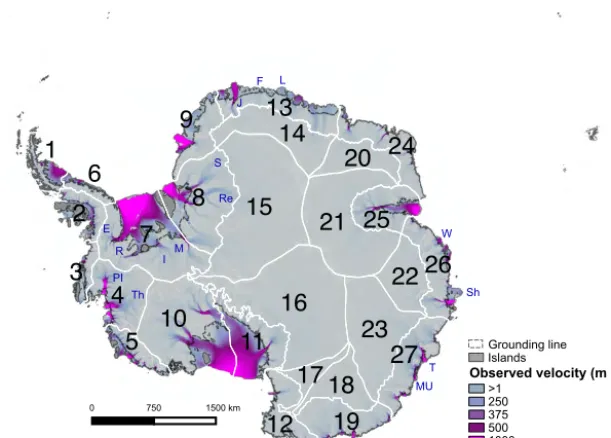
Figure 1.Observed surface velocity (m yr−1) in Antarctica, with geographic partitions in white, labeled with their corresponding numerical value (1–27). We indicate the observed grounding line with a dark gray dashed line and additional features of interest in blue: Th – Thwaites Glacier; PI – Pine Island Glacier; E – Evans Ice Stream; R – Rutford Ice Stream; I – Institute Ice Stream; M – Möller Ice Stream; Re – Recovery Ice Stream; S – Slessor Ice Stream; J – Jutulstraumen Glacier; F – Fimbul Ice Shelf; L – Lazarev Ice Shelf; W – West Ice Shelf; Sh – Shackleton Ice Shelf; T – Totten Glacier; MU – Moscow University Ice Shelf.
warming for all four sampling variables. For this purpose, we define geographic partitions (GPs), shown in white and num-bered 1 through 27 in Fig. 1. These partition boundaries are informed by analysis of various high-end warming scenar-ios and sensitivity studies (described below in Sect. 3.2) and represent a reconciliation of inferred spatial variability for all four sampled variables. More specifically, we first separate our partitions according to ice drainage basins. This choice respects the spatial correlation of ice flow and reflects general accumulation patterns over the ice sheet (Fyke et al., 2017). Finally, in order to distinguish among areas that may be af-fected by the presence of liquid water, we split the basins into regions above (plateau) and below (marine) the mean ice surface elevation of 2250 m. This is the elevation line be-low which we assume surface melt may be present by the end of the 21st century (i.e., Supplement figure in DeConto and Pollard, 2016). Such a division is also appropriate for ice shelf melt forcing, as extreme sensitivity experiments reveal that the grounding line rarely retreats beyond the present-day 2250 m surface elevation contour within the 100-year period investigated here (e.g., Fig. S5). Note that the above assump-tions, which we apply to the derivation of our partiassump-tions, are informed by past studies and general expert opinion; however for subsequent studies a different partition configuration may be deemed more appropriate. As the framework allows for various strategies, the choice of partitions should be an im-portant part of any future investigation, and the user should
specifically design his or her experiment based on the scien-tific questions being investigated.
For this study, every UQ sampling experiment is an en-semble of 800 forward simulations in total. With each exper-iment, every simulation is run for 100 years with a differ-ent combination of perturbed forcing in each partition. For repeatability, we seed all experiments identically, and there-fore any experiments with the same variable bounds and the same number of partitions impose identical sampling pertur-bations. Two-tailed statistics of output results, including dis-tributions of total and regional SLE contribution, are com-puted when all samples are completed. Note that for the stud-ies presented here, only sea level diagnostics at the end of the simulations are available. Therefore, we are restricted to the use of simulation final results and do not conduct any tempo-rally based analyses.
We launch each ensemble on the NAS Pleiades clus-ter, taking advantage of the parallelized ISSM core soft-ware as well as DAKOTA’s parallel management of ISSM sample simulations. Utilizing 1700 cpu’s, each ensemble of 800 ISSM simulations completes in less than 40 h.
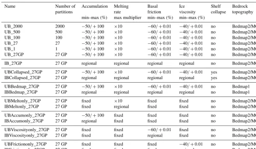
end-Table 1.List of sampling experiments and associated ranges of sampled variables for the UB and IB experiments. Here, we report all UB simulations. IB is marked as “regional” and is displayed in Table 2. Partitions are randomly generated, unless noted by GP, in which case they are geographically based. For ice shelf basal melt, the maximum bounds are given as melt multipliers, while all other variable bounds are given in percentage change. Minimum melt bounds within a partition are not represented here because they are not represented by a uniform value (see Table 2 and Sect. 3.1).
Name Number of Accumulation Melting Basal Ice Shelf Bedrock
partitions rate friction viscosity collapse topography
min–max (%) max multiplier min–max (%) min–max (%)
UB_2000 2000 −50/+100 ×10 −60/+0.01 −40/+0.01 no Bedmap2/MC
UB_500 500 −50/+100 ×10 −60/+0.01 −40/+0.01 no Bedmap2/MC
UB_100 100 −50/+100 ×10 −60/+0.01 −40/+0.01 no Bedmap2/MC
UB_27 27 −50/+100 ×10 −60/+0.01 −40/+0.01 no Bedmap2/MC
UB_1 1 −50/+100 ×10 −60/+0.01 −40/+0.01 no Bedmap2/MC
UB_27GP 27 GP −50/+100 ×10 −60/+0.01 −40/+0.01 no Bedmap2/MC
IB_27GP 27 GP regional regional regional regional no Bedmap2/MC
UBCollapsed_27GP 27 GP −50/+100 ×10 −60/+0.01 −40/+0.01 yes Bedmap2/MC
IBCollapsed_27GP 27 GP regional regional regional regional yes Bedmap2/MC
UBBedmap_27GP 27 GP −50/+100 ×10 −60/+0.01 −40/+0.01 no Bedmap1
IBBedmap_27GP 27 GP regional regional regional regional no Bedmap1
UBMeltonly_27GP 27 GP fixed ×10 fixed fixed no Bedmap2/MC
IBMeltonly_27GP 27 GP fixed regional fixed fixed no Bedmap2/MC
UBAccumonly_27GP 27 GP −50/+100 fixed fixed fixed no Bedmap2/MC
IBAccumonly_27GP 27 GP regional fixed fixed fixed no Bedmap2/MC
UBViscosityonly_27GP 27 GP fixed fixed −60/+0.01 fixed no Bedmap2/MC
IBViscosityonly_27GP 27 GP fixed fixed regional fixed no Bedmap2/MC
UBFrictiononly_27GP 27 GP fixed fixed fixed −40/+0.01 no Bedmap2/MC
IBFrictiononly_27GP 27 GP fixed fixed fixed regional no Bedmap2/MC
member, generalized for the entire AIS. In the second ap-proach, informed bounds (IB), variable bounds are specified for each GP. These regionally based bounds are informed by past sensitivity experiments or future emission scenario model runs, such that they represent a more realistic bound for future warming for each variable. We describe the UB and IB approaches and the strategy taken for determining the bounds for each sampling variable below, in Sect. 3.1 and 3.2, respectively.
In Table 1, we list all the UB and IB UQ experiments completed for this study. This table summarizes the partition scheme (number and type) used for each experiment as well as the range of values set for each forcing (ice shelf melt rate, accumulation, ice viscosity, and basal friction) or the geom-etry used (bedrock topography and ice shelves collapsed) in the experiment.
The first suite of UB experiments presented in Table 1 vary only by partition configuration. We conduct these first five experiments (UB_2000, UB_500, UB_100, UB_27, and UB_1; see Fig. S3) in order to illustrate how different num-bers of randomly generated equal-area partitions may affect the statistical distribution of the 100-year AIS SLE contribu-tion. Note that we run all of these experiments using the
con-trol simulation setup described in Sect. 2.3.1. In addition, we run a UB and an IB sampling experiment using the control simulation setup and the GP configuration (UB_27GP and IB_27GP, respectively) for comparison against the randomly generated partition experiments.
IBFrictiononly_27GP). This allows us to assess how each variable individually contributes to the total SLE distribution for the UB_27GP and IB_27GP sampling experiments.
3.1 Uniform bounds
For the UB experiment, we follow a typical sensitivity ap-proach to ice sheet model projections. Variable bounds do not vary regionally and are chosen largely to reflect changes in forcing that could result from large-scale warming of the climate over the next century. Here, we focus on exposing the system to a large range of plausible climate realizations to evaluate the model stability and feedbacks.
For accumulation, we set the minimum bound to a−50 % change and the upper bound to a+100 % change in the con-trol run accumulation forcing. The accumulation minimum bound represents the historical maximum annual variabil-ity in SMB over the last 200 years, as estimated from ice cores (Frezzotti et al., 2013). The upper bound is equivalent to the precipitation change expected due to an increase in surface temperature of about 10◦C, in accordance with the Clausius–Clapeyron relation (for current mean temperatures over the AIS). This value is representative of estimated accu-mulation changes in high-elevation areas of East Antarctica, but is likely an overestimate in the West AIS (Frieler et al., 2015).
For ice viscosity, we set the minimum bound to a−40 % change in ice viscosity used in the control run to account for an extreme decrease in ice viscosity due to cryo-hydrologic warming from increases in surface temperature and surface liquid water (rain and/or surface melt) (Schlegel et al., 2015). In the most extreme case, this assumes that surface ice tem-peratures reach the melting point of ice during the summer (from 5◦C warming along the margins to a 30◦C warming in the deep interior of the continent). In this case, surface water could percolate through the ice column and refreeze at depth, rapidly altering the ice thermal regime (Phillips et al., 2010, 2013). Where required, minimum bounds are restricted in order to ensure that all values remain above the viscosity of ice at melting point (Cuffey and Paterson, 2010). On float-ing ice, this bound also represents a change to the ice shelf rheology (i.e., damage) due to the percolation of surface melt into the floating ice and structural weakening (Borstad et al., 2012). As we do not consider increases to ice viscosity to be realistic, we set the maximum bound to the control run value plus 0.01 %.
For basal friction, we set the lower bound to a −60 % change in the values used in the control run, which is equiv-alent to the SeaRISE experiment S2 (Nowicki et al., 2013), i.e., a 2.5 times increase in sliding. We set the basal friction upper bound to the control run value plus 0.01 %.
For ice shelf basal melt rates, we do not set the lower bounds as a uniform change, but instead consider the in-terannual variability within each partition by setting it to the regional area-averaged percent difference between the
mean annual melt rate and the minimum annual melt rate. This change is generally small; i.e., for the GP configuration, the largest melt rate reduction is 0.1 m yr−1. For the upper bounds, we choose a multiplication factor of 10 times the control run melt rate, which for Pine Island Glacier repre-sents a grounding line potential temperature increase larger than 10◦C (considering the temperature dependency of Rig-not and Jacobs, 2002). While this factor represents a most extreme ocean forcing for warm ice shelves (e.g., Amundsen Sea), it is important to note that it also underestimates poten-tial warming in others (e.g., cold shelves like Filchner–Ronne Ice Shelf; Hellmer et al., 2012). This dichotomy illustrates the difficulty in designing an appropriate ice shelf melt rate perturbation experiment for Antarctica, as typically a single offset or multiplier value is chosen to represent a generalized warming experiment.
3.2 Informed bounds
In the IB experiment, we refine GMSL projections over the coming century by defining sampling bounds that are region-ally informed by model projections or targeted model sensi-tivity studies. All IB experiments are conducted on 27 GPs, and sampling variable bound ranges are determined sepa-rately for each partition.
IB lower bounds for ice shelf melt rates are the same as for UB. Upper bounds for ice shelf melt rates are deter-mined from MITgcm idealized sensitivity experiments (see Appendix Sect. A). All bounds for IB ice shelf melt rates are expressed as multiplication factors of the control run melt rate values (Table 2).
We base accumulation bounds on results from the Coupled Model Intercomparison Project Phase 5 (CMIP5) (Pachauri et al., 2014; Church et al., 2013), using results from the 80 publicly available RCP8.5 emissions scenario (Taylor et al., 2012) atmospheric simulations to characterize possi-ble future spread in AIS precipitation change over the next century due to high greenhouse gas emission warming. The upper and lower IB are set respectively as the maximum and minimum percent simulated accumulation change, with con-sideration to output from the 80 CMIP5 models, between the mean of the years 2006–2010 and 2096–2100.
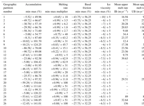
Table 2.For the IB experiments, the associated range of sampled variables for each GP is shown (Fig. 1). The last two columns list the mean upper-bound ice shelf melt rates forced for each marginal partition during the sampling experiments, for IB and UB. The mean upper-bound melt rate is equal to the maximum melt rate multiplier times the control ice shelf melt rate values, with area averaged over the initialization ice shelf area within each margin partition.
Geographic Accumulation Melting Basal Ice Mean upper Mean upper
partition rate friction viscosity melt rate melt rate
number min–max (%) min–max multiplier min–max (%) min–max (%) IB (m yr−1) UB (m yr−1)
1 −5.52/+49.96 ×0.65/×18 −43.75/+56.25 −10/+5 16.94 9.4
2 −49.72/+66.67 ×0.99/×3.5 −43.75/+56.25 −8/+5 9.77 27.7
3 −30.70/+57.19 ×0.99/×6.2 −43.75/+56.25 −7/+5 20.28 32.8
4 −29.50/+66.76 ×0.99/×1.8 −43.75/+56.25 −8/+5 20.83 118.3
5 −58.34/+71.60 ×0.99/×2.7 −43.75/+56.25 −6/+5 9.48 34.8
6 −5.00/+54.77 ×0.75/×40 −43.75/+56.25 −8/+5 34.4 8.6
7 −8.31/+87.60 ×0.35/×63.2 −43.75/+56.25 −6.5/+5 23.37 3.7
8 −10.82/+101.70 ×0.98/×31 −43.75/+56.25 −6.5/+5 12.4 4
9 −10.23/+124.25 ×0.83/×45.7 −43.75/+56.25 −6/+5 17.38 3.8
10 −86.58/+78.68 ×0.41/×15.1 −43.75/+56.25 −8.5/+5 23.56 15.6
11 −90.72/+89.08 ×0.22/×15.1 −43.75/+56.25 −6/+5 23.56 15.6
12 −47.63/+111.00 ×0.93/×5 −27.75/+32.25 −5/+5 9.75 19.5
13 −23.86/+92.58 ×0.94/×62.9 −27.75/+32.25 −7.5/+5 39.63 6.3
14 −5.00/+104.42 ×0.99/×62.9 −27.75/+32.25 −5/+5 – –
15 −5.00/+91.95 ×0.99/×31 −27.75/+32.25 −5/+5 – –
16 −46.15/+107.71 ×0.99/×15.1 −27.75/+32.25 −5/+5 – –
17 −5.00/+105.93 ×0.99/×20 −27.75/+32.25 −5/+5 – –
18 −25.57/+86.78 ×0.99/×11.8 −27.75/+32.25 −5/+5 – –
19 −73.31/+97.52 ×0.96/×11.8 −27.75/+32.25 −6/+5 29.51 25.1
20 −59.29/+154.64 ×0.99/×100 −27.75/+32.25 −5/+5 − –
21 −5.00/+111.61 ×0.99/×51 −27.75/+32.25 −5/+5 – –
22 −8.12/+99.33 ×0.99/×172.2 −27.75/+32.25 −5/+5 – –
23 −5.00/+120.22 ×0.99/×7 −27.75/+32.25 −5/+5 – –
24 −53.61/+122.85 ×0.99/×100 −27.75/+32.25 −6.5/+5 89 8.9
25 −32.24/+146.85 ×0.87/×51 −27.75/+32.25 −6.5/+5 32.64 6.4
26 −12.45/+141.01 ×0.88/×100 −27.75/+32.25 −6.5/+5 156 15.6
27 −19.23/+139.85 ×0.99/×7 −27.75/+32.25 −6.5/+5 26.84 38.4
CMIP5 ice sheet model simulations under the RCP8.5 sce-nario (see, e.g., Supplement figure in DeConto and Pollard, 2016) such that, depending on the amount of meltwater sim-ulated within a specific partition by year 2100, ice viscosity lower bounds range from−10 % to−6 % change.
For basal friction, uncertainties are not well defined, and associated processes are part of an active field of research. For the Greenland Ice Sheet, surface runoff reaches the base of the ice sheet, and basal sliding increases or decreases, depending on the type of subglacial drainage system devel-oped (Bell, 2008; Sundal et al., 2011). In Antarctica, a lim-ited amount of supraglacial water is available to impact basal conditions, as most subglacial water is linked to basal heating (due to geothermal heat flux and frictional heat, i.e., Pattyn, 2010; Seroussi et al., 2017a) and is not directly affected by climate change. Consequentially, model errors in basal slid-ing can be mainly attributed to uncertainties in the inferred basal friction. We characterize this uncertainty by comparing the inferred basal friction from ISSM AIS models initialized
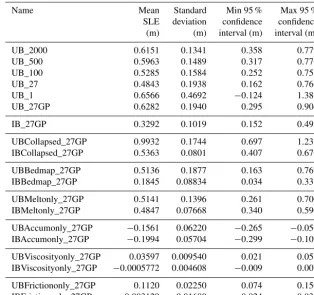
Table 3.SLE (m) and associated statistics resulting from 800 simulations for each of the experiments described in Table 1.
Name Mean Standard Min 95 % Max 95 %
SLE deviation confidence confidence
(m) (m) interval (m) interval (m)
UB_2000 0.6151 0.1341 0.358 0.779
UB_500 0.5963 0.1489 0.317 0.776
UB_100 0.5285 0.1584 0.252 0.758
UB_27 0.4843 0.1938 0.162 0.766
UB_1 0.6566 0.4692 −0.124 1.386
UB_27GP 0.6282 0.1940 0.295 0.904
IB_27GP 0.3292 0.1019 0.152 0.495
UBCollapsed_27GP 0.9932 0.1744 0.697 1.235
IBCollapsed_27GP 0.5363 0.0801 0.407 0.676
UBBedmap_27GP 0.5136 0.1877 0.163 0.767
IBBedmap_27GP 0.1845 0.08834 0.034 0.331
UBMeltonly_27GP 0.5141 0.1396 0.261 0.700
IBMeltonly_27GP 0.4847 0.07668 0.340 0.590
UBAccumonly_27GP −0.1561 0.06220 −0.265 −0.056
IBAccumonly_27GP −0.1994 0.05704 −0.299 −0.109
UBViscosityonly_27GP 0.03597 0.009540 0.021 0.052
IBViscosityonly_27GP −0.0005772 0.004608 −0.009 0.007
UBFrictiononly_27GP 0.1120 0.02250 0.074 0.150
IBFrictiononly_27GP 0.003129 0.01680 −0.024 0.032
4 Results
The goal of this study is to use sampling analysis to quan-tify the uncertainty in simulated SLE contribution from the AIS over a 100-year period. We also investigate how this un-certainty varies regionally. SLE contribution is determined by the change in ice volume above floatation during the 100-year simulation period, compared to the change in ice volume above floatation during the 100-year control run.
Our UQ results are presented in a number of formats. Distribution plots represent the probability density function (PDF) for the frequency of SLE contribution from Antarc-tica for the 800 independent random samples at the end of a 100-year-long forward simulation. In addition, all AIS con-tinental SLE contribution results are summarized in Table 3. To aid in regional analysis, bar plots represent the mean and standard deviation of SLE contribution from the sample sim-ulations for every GP.
4.1 Impact of partition choice
For this type of resource-limited UQ study, experimental de-sign is likely to impact the distribution and magnitude of the AIS SLE contribution, particularly the choice of parti-tion configuraparti-tion. To investigate this effect, we run a suite of UB experiments (such that for each of the four variables synchronously sampled, the sampling bounds are the same
for every partition), altering only the partition configurations (see Fig. S3). The experiments consist of a single-partition sampling, plus four experiments that are run with various numbers of randomly generated partitions (Table 1). Addi-tionally, we include an experiment with GP partitioning (see Sect. 2.4).
in-−1 −0.5 0 0.5 1 1.5 2 2.5 3 0
0.5 1 1.5 2 2.5 3 3.5 4
m SLE
Frequency
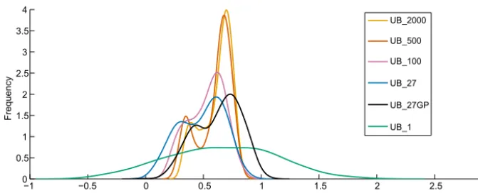
UB_2000 UB_500 UB_100 UB_27 UB_27GP UB_1
Figure 2.PDF of Antarctica SLE (m) contribution after 100 years, for 800 individual simulations sampled with UB and various partition configurations. The distribution results are from sampling experiments in which we vary the number and configuration of the sampling regions (partitions) (comparing experiments UB_2000, UB_500, UB_100, UB_27, UB_1, and UB_27GP). See Fig. S3 for plots of the spatial configuration of partitions for these experiments. See Table 3 for statistics relating to each curve.
creased numbers of samples (not shown) suggests that with LHS uniform sampling, 800 samples are adequate and that the resulting PDF curves shown here are robust. That is, our UB and IB PDF curves converge within 800 samples, with PDF means and spreads varying by less than 0.6 % beyond 800 samples. Indeed, the resulting spread is partly dictated by the fact that, while the number of partitions increases, the PDF curves for the total mass forcing (specifically the total continental SMB and total basal melt) tend to become more normally distributed and begin to narrow (a phenomenon dic-tated by the law of large numbers and the central limit theo-rem). After further analysis, we also find that such variations in spread can be contributed to dynamic feedbacks among the partitions. For instance, while UB_1 assumes that forcing of climatically driven parameters would change uniformly over the entire ice sheet, UB_2000 assumes minimal spatially proximate correlation. That means that with many partitions it is less likely that all partitions of the ice sheet will change together to promote mass gain or mass loss. Specifically, for a particular sample simulation, it is more likely that at least one partition within a drainage basin is promoting ice gain while the rest of the basin partitions are promoting ice loss. In this case, the one partition promoting ice gain may stall or counteract mass loss within the entire basin, making the occurrence of an end-member sample result even more rare as the number of sampling partitions increases.
Table 3 and Fig. 2 illustrate the effect of choosing parti-tions that promote spatial correlation (i.e., correlation within ice flow basin and by surface elevation), in contrast to the randomly generated partition distributions. The distributions of UB_27GP and UB_27GP are almost equivalent in stan-dard deviation and frequency, but the UB_27GP is shifted ap-proximately 0.14 m SLE to the right, indicating that the GP run is more likely to lose mass than the run with randomly generated partitions. The GP configuration respects ice flow boundaries on the 100-year timescale considered here and
therefore does not bisect large glaciers or ice streams, as the randomly generated partitions are likely to do (e.g., Pine Is-land Glacier; Fig. S3). Within the GP configuration, large glaciers and ice streams in the same basin change syn-chronously (uniformly with respect to each independently sampled variable), which is likely to promote glacier insta-bility and ice mass loss. Consequently, we choose to utilize the GP configuration for all other UQ experiments presented in this paper, as sampling with this configuration is represen-tative of physically based correlations within the ice sheet system not captured by randomly generated partitions.
One important characteristic of the partition experiment distributions is that, for the random (equal area) experiments, the distribution mean shifts to the left with the use of fewer partitions (Fig. 2). This phenomenon occurs in response to the sampling of accumulation, which is directly responsible for dictating the amount of mass that is added to the ice sheet (Fig. 3). The lower the number of partitions, the larger the partition regions, and the more likely increases in accumu-lation will affect a significant portion of the AIS. Forcing a larger ice sheet area with significant increases in accumula-tion (up to 100 %) results in mass storage, encouraging the ice sheet to grow and negatively affecting SLE contribution. Therefore, when running with a smaller number of larger sized partitions, the simulations are more likely to gain mass, resulting in a SLE PDF shift to the left.
4.2 Uniform bounds experiments
(UB-−0.4 −0.2 0 0.2 0.4 0.6 0.8 1 1.2 1.4 0
5 10 15 20 25 30 35 40 45
m SLE
Frequency
UB_27GP UBMeltonly_27GP UBAccumonly_27GP UBViscosityonly_27GP UBFrictiononly_27GP
UB individual variable PDFs summed
(a)
a
−0.4 −0.2 0 0.2 0.4 0.6 0.8 1 1.2 1.4
0 5 10 15 20 25 30 35 40 45
m SLE
Frequency
(b)
a
IB_27GPIBMeltonly_27GP IBAccumonly_27GP IBViscosityonly_27GP IBFrictiononly_27GP
IB individual variable PDFs summed
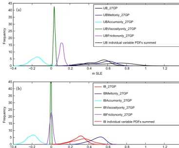
Figure 3.PDF of SLE from ensemble runs with 800 simulations using GP partitioning for sampling variables in combination and
individ-ually. Both the(a)UB (solid black line) and(b)IB (solid red line) experiments are included. Variables ice shelf basal melt, accumulation,
ice viscosity, and basal friction are sampled together randomly (UB_27GP, IB_27GP). Curves of other colors represent the sampling of each variable individually: ice shelf basal melt (UBMeltonly_27GP, IBMeltonly_27GP: dark blue), accumulation (UBAccumonly_27GP, IBAccu-monly_27GP: cyan), ice viscosity (UBViscosityonly_27GP, IBViscosityonly_27GP: dark green), and basal friction (UBFrictiononly_27GP,
IBFrictiononly_27GP: purple). Hash-marked curves represent the sums of the individual variable curves, for(a)UB (black) and(b)IB (red).
See Table 3 for statistics relating to each curve.
Meltonly_27GP) isolates this variable as the only source with a bimodal distribution (Figs. 3a and S4). By sampling ice shelf melt rates alone, we remove the feedbacks from the other sampled variables. This feedback is nontrivial, as evidenced by the difference between the variable summed and the combined sampling curve in Fig. 3a. It is clear that for our UB runs, ice shelf melt is responsible for the majority of the spread (Table 3 and Fig. 3a) as well as for the bimodal behavior of the UB distributions (Fig. S4).
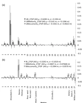
Additional regional analysis pinpoints the Amundsen Sea (GP 4) as the dominant source of the AIS uncertainty (Fig. 4), suggesting that the large ice shelf melt rates forced in this area are almost entirely responsible for the spread of the to-tal AIS PDF (Fig. 4). These results agree with those from past model sensitivity experiments and projection-based AIS warming scenario simulations that have reported complex grounding line and ice dynamic responses within the Amund-sen Sea (e.g., Cornford et al., 2015; Ritz et al., 2015). Un-der the UB experiment, we find that the mean SLE
con-tribution from the Amundsen Sea is 297 mm, accounting for about 47 % of the continental AIS mean SLE contribu-tion and about 89 % of its uncertainty (difference between the maximum and minimum 95 % confidence intervals). The forcing of ice shelf melt rates alone accounts for 82 % of the Amundsen Sea’s mean SLE response and about 72 % of its uncertainty (Fig. 4).
Other regions responsible for SLE contribution are GP 27 (Wilkes Land coast, including Totten Glacier and Moscow University Ice Shelf) and GP 7 (the Ronne Ice Shelf basin, particularly Institute and Möller ice streams) (Fig. 4). Single sensitivity runs forced with end-member warming bounds in-dicate that western Ross Ice Shelf–Siple Coast (GP 10) is also expected to be a larger contributor to SLE on timescales longer than considered here (∼200 years, Fig. S6).
4.3 Informed bounds experiments
-‐0.1 -‐0.05 0 0.05 0.1 0.15 0.2
1 2 3
Amu
nd
sen
S
. -‐
4 5 6
Ro
nn
e
-‐
7
Filc
hne
r -‐ 8
9
R
o
ss
we
st
-
1
0
Ro
ss
ea
st
-‐
1
1 12
Fi
m
bu
l /
L
azar
ev
-‐
1
3 14 15 16 17 18
D'
U
rv
ille
S. -‐ 19
20 21 22 23 24
Amery
-‐
25
D
av
is
S
. -‐
2
6
W
ilk
es
L
an
d
-‐
27
m S
LE
Region
IB_27GP (AIS μ = 0.3292 m, σ = 0.1019 m)
IBMeltonly_27GP (AIS μ = 0.4847 m, σ = 0.07668 m) IBAccumonly_27GP (AIS μ = -‐0.1994 m, σ = 0.0570 m)
-‐0.1 -‐0.05 0 0.05 0.1 0.15 0.2 0.25 0.3 0.35 0.4 0.45 0.5
1 2 3 4 5 6 7 8 9 10 11 12 13 14 15 16 17 18 19 20 21 22 23 24 25 26 27
m S
LE
UB_27GP (AIS μ = 0.6282 m, σ = 0.194 m) UBMeltonly_27GP (AIS μ = 0.5141 m, σ = 0.1396 m) UBAccumonly_27GP (AIS μ = -‐0.1561 m, σ = 0.0622 m) (a)
(b)
Figure 4.Mean SLE (m) and standard deviation bounds for ensemble runs with 800 simulations using GP partitioning, presented regionally,
comparing results from the sampling of a combination of variables, of only ice shelf basal melt rates, and of only surface accumulation (a,
UB;b, IB). Numbers correspond to GP numbers (see Fig. 1). Mean (µ) and standard deviation (σ) SLE for the total ice sheet are indicated
in the legend for each sampling experiment.
sampling bounds compared to the control run vary region-ally for each parameter in the IB experiments. In contrast to the UB experiments, the IB experiments encompass realiza-tions that are foreseeable according to the literature, sensitiv-ity experiments, and CMIP5 ensemble mean projections for the end of the century (see Sect. 3.2). Under these restric-tions, the IB experiment results are still dominated by the ice shelf melt rate forcing (Fig. 3). Also similar to the UB experiments, the effects of increased ice shelf melt rates are mitigated by increases in accumulation (the most important variable after melt rates). Basal friction and ice viscosity play minor roles in the resulting SLE distributions, as over the 100-year period we do not expect surface runoff to increase substantially enough to affect these parameters on a basin
scale. In the UB experiments, in which Amundsen Sea ice shelf melt is the most significant contributor, the maximum bounding melt rate is equivalent to a 10 times multiplier of the control melt rates. Overall, we do not consider this value realistic for the Amundsen Sea sector (GP 4, Fig. 1) over the next century, especially since melt rates in this area are already substantially greater than melt rates for the rest of the AIS (i.e., warm ocean waters currently reach the largest glaciers in the region).
ac-celeration already observed in the West AIS during the last decade (Shepherd et al., 2018). However, the most extreme IB simulations reveal that an addition of 66 mm of SLE con-tribution from the Amundsen Sea is plausible in response to 100 years of perturbed forcing (Fig. 4). This response repre-sents an acceleration of about 3 times the present-day rate of mass loss in this region (Medley et al., 2014). We find that with respect to the total AIS SLE potential contribution un-der the IB experiment, the Amundsen Sea is a relatively mi-nor contributor to future sea level rise (Fig. 4). It is conceiv-able that warm waters reach the continental shelf, heating the ocean waters beneath traditionally cold ice shelves, and sig-nificantly increasing the ice shelf melt potential within these current regions of low melt rates (Hellmer et al., 2012). Our ocean model sensitivity studies (Sects. 3.2 and A) reveal a similar warming potential beneath the Ronne Ice Shelf, re-sulting in relatively large end-member melt rates for our IB experiments (Table 2). As a result, we find that the most sig-nificant potential contributors are ice streams feeding Ronne Ice Shelf (GP 7), particularly the Evans and Rutford ice streams (Fig. S5c) as well as the Institute and Möller ice streams, together resulting in a 161 mm mean SLE contri-bution (∼50 % of the total AIS contribution). The SLE con-tributions from these ice streams are dominated by ground-ing line retreat forced by prescribed ice shelf melt rates, and therefore these results are direct consequences of the large upper-bound multiplier chosen for GP 7 (Table 2). In this case, ice shelf melt alone is responsible for approximately all of the mean response for this region and 82 % of its uncer-tainty (Fig. 4).
Other contributing regions include GP 8 (Filchner Ice Shelf basin: Slessor and Recovery ice streams), GP 10 (west-ern Ross Ice Shelf: Siple Coast), GP 13 (including Jutul-straumen Glacier, Fimbul and Lazarev ice shelves), and GP 25 (Amery Ice Shelf basin) (Fig. 4). Note that results from single-simulation sensitivity runs forced with IB end-member warming bounds indicate that under the IB experi-ment the Amundsen Sea may be a more significant contrib-utor to SLE on a timescale beyond the 100 years considered here (Fig. S6), as suggested by other regionally based AIS modeling experiments (Cornford et al., 2015). Of additional interest are GP 26 and GP 27. Within these regions, ice shelf melt IB simulations allow for potential SLE contributions similar to those listed above; however, accumulation bounds in these regions are substantial enough to counterbalance ice that is potentially lost to elevated ice shelf basal melt rates (Fig. 4) (up to an upper bound of 140 % increase in accumu-lation, Table 2). This leads to large uncertainties within these regions around a lower mean SLE contribution that would be much higher if melt were sampled alone.
4.4 Impact of ice shelf collapse
As our simulations do not include migrating ice fronts, and therefore subsequent reduction in ice shelf buttressing, they
may underestimate future sea level rise. To quantify the effect of back stress provided by the current ice shelves, we conduct sampling experiments on a control run that instantaneously loses all of its current ice shelves at the beginning of the run (see Sect. 2.3.2). While the removal of ice shelves does not affect SLE contribution directly (ice shelves are floating), it eliminates any buttressing of the interior ice that is provided by the current ice shelves.
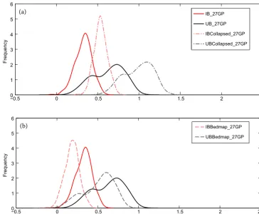
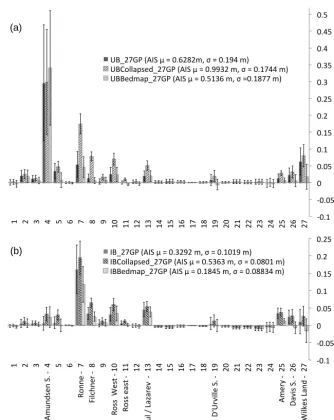
Figure 5a shows the UBCollapsed_27GP and IBCol-lapsed_27GP experiments’ SLE PDFs as well as the UB_27GP and IB_27GP experiments’ SLE PDFs. Generally, we find that the effect of collapsing AIS ice shelves creates an additional SLE contribution of 0.37 and 0.32 m for UB and IB experiments, respectively. In addition, experiments including initial ice shelf collapse show a small narrowing in their uncertainty ranges (Fig. 5a and Table 3). It is clear that the regions most affected are those with the largest ice shelves, and therefore the most buttressing. The areas signif-icantly affected include GP 7 and GP 8 (the Filchner–Ronne basin), GP 10 (western Ross Ice Shelf), and GP 13 (Dronning Maud Land coast, including Fimbul and Lazarev ice shelves). Other sensitive regions of minor note include GP 5, GP 25, and GP 26 (Fig. 6).
For the regions noted above, we find that the standard deviation is reduced for the collapsed ice shelf experiment (Fig. 6). This is indicative of the loss of a number of lower-bound sample runs in which grounding line retreat is mit-igated. Indeed, once the ice shelves are instantaneously re-moved, these areas are already committed to SLE contribu-tion in response to the removal of present-day ice shelf but-tressing. This is particularly pertinent in the case of the large cold Filchner–Ronne and Ross ice shelves, where the col-lapsed ice shelf SLE contribution is comparable between the UB and IB experiments (means within 1σ), even though their melt rate upper bounds have drastically different values (Ta-ble 2). Such results highlight the importance of the role of ice shelf buttressing in the stability of the glaciers that feed into cold ice shelf regions. Indeed, our results represent a lower bound on the effects of future ice shelf collapse since ice margins do not migrate through time.
4.5 Impact of bedrock topography
−0.5 0 0.5 1 1.5 2 2.5 0
1 2 3 4 5 6
Frequency
(a)
−0.5 0 0.5 1 1.5 2 2.5
0 1 2 3 4 5 6
m SLE
Frequency
(b)
IB_27GP UB_27GP IBCollapsed_27GP UBCollapsed_27GP
IBBedmap_27GP UBBedmap_27GP
Figure 5.PDFs of SLE resulting from ensemble runs with 800 simulations using GP partitioning, comparing the effects of using different
boundary forcing.(a)Curves resulting from sampling of UB (UB_27GP, black) and IB (IB_27GP, red) experiments, compared with results
from runs forced with the collapse of all Antarctic ice shelves at the beginning of the simulation (dash-dot) (UBCollapsed_27GP and
IBCollapsed_27GP).(b)Plot similar to(a)but with additional ensemble runs showing the impact of using a bedrock topography (dashed)
derived from Bedmap1 (UBBedmap_27GP and IBBedmap_27GP). See Table 3 for statistics relating to each curve.
while for the IB experiment, the IBBedmap_27GP and IB_27GP means differ beyond a standard deviation (Fig. 5 and Table 3). Overall, the improvement from Bedmap1 to Bedmap2/MC results in a right shift of 0.11 m for the UB experiments and 0.14 m for the IB experiments. Both experi-ments reveal a slight widening of uncertainty bounds with the change from Bedmap1 to Bedmap2/MC (with an increase in uncertainty of 18 % and 1 % for IB and UB, respectively), suggesting that the improved bedrock topography results in an increase in the sample space of possible grounding line re-treat realizations as well as a widening of the tails (Fig. 5b).
Regional analysis reveals that the quality of the bedrock topography affects the rate of retreat of spe-cific glaciers, depending on the forcing. For instance, in the UBBedmap_27GP experiment, the Amundsen Sea con-tributes 15 % (or 44 mm) more SLE than does the UB_27GP experiment (Fig. 6). Yet, for the UB Bedmap1 experiments overall, we find that regional decreases in mass loss (particu-larly in the East AIS) outweigh the Amundsen Sea mass loss increases. The area with the largest mass loss decrease due to the Bedmap1 topography is GP 27 (Wilkes Land coast, including Moscow University Ice Shelf and Totten Glacier;
Fig. 6), contributing a mean of 26 and 46 mm less to GMSL over the 100-year simulation for IB and UB, respectively. For the IB experiment, in all regions IBBedmap_27GP con-tributes less SLE than does IB_27GP (Fig. 6). In particular, GP 26 and GP 27 are affected by the different bedrock topog-raphy maps, as is the largest SLE contributor, GP 7 (Ronne Ice Shelf) (Fig. 6).
-‐0.1 -‐0.05 0 0.05 0.1 0.15 0.2 0.25
1 2 3
Amu
nd
sen
S
. -‐
4 5 6
Ro
nn
e
-‐
7
Filc
hne
r -‐ 8
9
R
o
ss
W
es
t
-
1
0
Ro
ss
ea
st
-‐
1
1 12
Fi
m
bu
l /
L
azar
ev
-‐
1
3 14 15 16 17 18
D'
U
rv
ille
S. -‐ 19
20 21 22 23 24
Amery
-‐
25
D
av
is
S
. -‐
2
6
W
ilk
es
L
an
d
-‐
27
m S
LE
Region
IB_27GP (AIS μ = 0.3292 m, σ = 0.1019 m) IBCollapsed_27GP (AIS μ = 0.5363 m, σ = 0.0801 m) IBBedmap_27GP (AIS μ = 0.1845 m, σ = 0.08834 m)
-‐0.1 -‐0.05 0 0.05 0.1 0.15 0.2 0.25 0.3 0.35 0.4 0.45 0.5
1 2 3 4 5 6 7 8 9 10 11 12 13 14 15 16 17 18 19 20 21 22 23 24 25 26 27
m S
LE
UB_27GP (AIS μ = 0.6282m, σ = 0.194 m)
UBCollapsed_27GP (AIS μ = 0.9932 m, σ = 0.1744 m) UBBedmap_27GP (AIS μ = 0.5136 m, σ =0.1877 m)
(a)
(b)
Figure 6.Same as Fig. 4 but comparing the combined variable GP experiments, the combined variable GP experiments with ice shelves
collapsed, and the combined variable GP Bedmap1 experiments (a, UB;b, IB).
5 Discussion
Model projections of future sea level rise are inherently un-certain and depend largely on the model boundary condi-tions and climate forcing. Ice sheet models are specifically designed to capture the complex dynamic responses to ocean and atmospheric change, compounding the difficulty of pin-pointing the potential sources of model uncertainty. Here, we uniquely take advantage of the ISSM–DAKOTA UQ frame-work, which allows for a relatively high spatial resolution near shear margins and the grounding line, a feature advan-tageous for the physical modeling of ice flow and ground-ing line retreat and an improved representation of bedrock topography. Because ISSM also has the option of running with various stress balance approximations, the experimental
design described here takes advantage of a two-dimensional representation of ice flow that reasonably replicates results from a more complex stress balance model (Fig. S2 and Sect. 2.3.1). Thus, the ISSM–DAKOTA highly parallelized, high-resolution UQ framework allows for continental and re-gional statistical assessment of AIS dynamic mass change.
complexity of grounding line response. Furthermore, we find grounding line retreat is locally enhanced when the simula-tion is forced by a simultaneous reducsimula-tion in basal fricsimula-tion, ice viscosity, or accumulation (i.e., a mean enhancement of 12 % for IB and 19 % for UB experiments when all variables are combined, Fig. 3), which is a source of added complexity in our results. Indeed, the response of the grounding line po-sition to increased ice shelf basal melt rate forcing is strongly dependent on the applied melt rate as well as the local condi-tions, particularly bedrock geometry and ice shelf buttress-ing, which determine grounding line stability. This means that the resulting SLE PDFs are not only a ramification of forcing, boundary conditions, and input parameters, but also a combined consequence of various regional responses of many individual glaciers.
These results suggest that, in particular, it is most impor-tant to reduce uncertainty in the representation of grounding line migration and in ice shelf basal melt rate forcing. In the experiments presented here, we utilize an optimized recon-struction of historical melt rates from an ocean model run at a horizontal grid spacing of 9 km, and for the ice sheet model areas of floating ice are restricted to a horizontal reso-lution of 8 km or finer with coarser grid spacing upstream of the grounding line. For the ocean model, the resulting grid is an improvement over past studies in terms of resolv-ing the circulation beneath key ice shelves (Schodlok et al., 2016), but those areas with smaller outlet glaciers and ice shelves still require finer grid spacing. These areas include Enderby Land (GP 24) and the George V Land–Davis Sea sector (GP 26), whose melt rates remain highly uncertain (Tables 2 and S1 and Appendix Sect. A). For the ice sheet model, the resolution used here is also improved over previ-ous continental-scale studies (Ritz et al., 2015; DeConto and Pollard, 2016; Pattyn, 2017); yet in order to properly model grounding line migration, the ice sheet model should still be run with a horizontal resolution finer than 8 km near the present-day grounding line (Durand et al., 2009; Gladstone et al., 2010; Seroussi et al., 2014a). Due to computational re-strictions, the horizontal mesh resolution of both the ocean and ice sheet model used here are restricted to values coarser than desired, especially in the interior, where the grounding line migrates into regions with resolutions even lower than 8 km (Figs. S1 and S5). Currently, finer resolutions can be accomplished with the use of regional-scale models; but ide-ally, future improvements would include coupling of highly resolved continental-scale ocean and ice sheet models, in lieu of parameterizations, in order to best represent the evolu-tion of melt rates as grounding lines migrate in the future. A coupled ocean–ice sheet model capable of resolving im-portant topographical features may improve the estimates of melt rates beneath ice shelves as grounding lines retreat by simulating the evolution of the shape of the cavity between the ice shelves and the bedrock topography. Indeed, by rep-resenting the physical changes in ocean circulation patterns beneath new ice shelves, the models are expected to produce
more credible estimates of ice shelf melt rates (De Rydt and Gudmundsson, 2016; Seroussi et al., 2017b).
In order to better assess the impact of mesh resolution on the uncoupled ice sheet model simulations used here, we conducted sensitivity experiments on a regional model of Thwaites Glacier (Seroussi et al., 2017b). Results suggest that the ISSM mesh resolutions are sufficient to capture the general behavior that the same model would produce with a 4 times finer spatial resolution. Additional experiments con-ducted on a lower-resolution ISSM AIS (in which the finest model spatial resolution is 3 km instead of the 1 km used in this study) illustrate how model resolution can affect the con-tinental AIS model response in a complex way (Fig. S4). More specifically, we find that the lower-resolution model results reveal a slight decrease in SLE AIS contribution for the IB experiments and an increase for the UB experiments. For the UB experiment, this increase is a direct consequence of how mesh resolution affects the model response to ice shelf melt rates (Fig. S4), in agreement with results from Pat-tyn (2017) on a 100-year timescale using coarser simulation meshes. Results on the basin scale (not shown) reveal that the difference between the higher- and lower-mesh-resolution models are distinctively attributed to the dynamic behavior of the ice streams feeding the Filchner–Ronne ice shelves, the Amundsen Sea sector, and Wilkes Land. More specifically, higher resolution promotes grounding line stability in all of these regions for the UB experiments and particularly pro-motes instability in Pine Island Glacier, Moscow University Ice Shelf, and Totten Glacier for the IB experiments. Since the IB upper-bound ice shelf melt forcing is less extreme than that of the UB forcing for Pine Island and Wilkes Land, the final grounding line position after 100 years falls within re-gions of locally complex topography (Fig. S5). As a result, the IB experiments emphasize more complicated feedbacks between bedrock geometry and grounding line dynamics. These findings suggest that improved resolution within these basins generally affects model results by refining the bedrock topography, altering stability, and changing the threshold for collapse. Thus, sea level projections are highly dependent on the accuracy of the bedrock topography beneath both the cur-rent and any new ice shelf areas.
re-treat. For example, we find that the largest regional impact of bed topography is in the Amundsen Sea sector under the UB experiment (GP 4, Fig. 6). In this region, the use of Bedmap1 promotes greater regional SLE contribution, yet on a continental scale the Bedmap1 topography results in a re-duced total AIS SLE contribution. Such findings highlight the need for continual improvement of high-resolution maps of bedrock topography, prioritization of long-term measure-ments of melt rates and ocean temperatures, and the ability for models to capture increased details of the bedrock (partic-ularly in areas near the present and potential future ground-ing line positions, includground-ing the Amundsen Sea sector, the Filchner–Ronne Ice Shelf basin, and coastal Wilkes Land).
While ice shelf melt rates are an important source of uncer-tainty in the SLE contribution from the AIS, regional results for the IB experiments also highlight the potential for accu-mulation changes to significantly affect results, particularly in the East AIS. Notably, we find that the Davis Sea sector and Wilkes Land coast (Fig. 4, GP 26 and GP 27, including Moscow University Ice Shelf, Totten Glacier, West Ice Shelf, and Shackleton Ice Shelf) are subject to potential increases in accumulation that can be large enough to mitigate the mass loss resulting from grounding line retreat forced by greater ice shelf melt rates. In these regions, enhanced accumulation can counteract any melt-induced SLE contribution and also widens the simulation uncertainty (Fig. 4). These results sug-gest that in these coastal areas of the East AIS, the modeling of future ice mass change may be too uncertain to even de-termine its sign. As a result, it will be necessary to properly model atmospheric forcing and its response to warming (in-cluding refinement of ice sheet and ocean model resolution), particularly within the Wilkes Land (GP 27), Queen Mary Land, and Wilhelm II Land regions (GP 26), in order to re-duce uncertainty in future sea level projections.
As the results illustrate, simulations are highly sensitive to oceanic and atmospheric forcing; thus care must be taken to understand how experimental design affects uncertainty. For instance, for the UQ sampling experiments, uncertainty is sensitive to the partitioning methods used (Fig. 2 and Ta-ble 3), so our results are a function of our partition boundaries and their chosen bounds. While we consider our adoption of the GP configuration a reasonable approach, this assump-tion is a model limitaassump-tion. More specifically, our results sug-gest that the design of partition configuration requires knowl-edge about proximal correlations in model forcing associated with changes in climate. For instance, if we underestimate regional correlation by using multiple partitions, this choice may, for accumulation, overestimate the mean of the SLE response distribution and, for ice shelf melt rates, underes-timate the SLE uncertainty (or probability of end-member occurrence). Our method also assumes that our sampling variables can be sampled independently, though in actuality there are physical relationships that dictate these variables may vary together in response to warming. For example, cli-mate warming is generally associated with increased ice shelf
basal melt rates, increases in accumulation, and decreases in ice viscosity and basal friction. Ideally, our UQ experi-ments would consider these relationships; however we can-not adequately accommodate them into our present experi-mental design, especially since the quantification of such re-lationships is highly uncertain in itself. Therefore, in order to characterize and bound how spatial and variable correlation could affect our results, we conduct additional UQ sensitiv-ity experiments that assume definitive correlations between all variables and within all partitions for all samples. Ulti-mately, these experiments reveal the magnitude of this effect is dependent on the experiment being conducted and partic-ularly on the sampling bounds of the forcing variables. For instance, results suggest that for the IB GP experiment, im-posed continental-wide spatial and variable correlations can decrease the maximum 95 % confidence interval by up to 120 mm. Yet, for the UB GP experiment, imposed correla-tions can widen the SLE PDF uncertainty bounds, increas-ing the maximum 95 % confidence interval by up to 172 mm. Such results illustrate the sensitivity and complexity of the system being assessed. Indeed, it is important to note that in the future, the precise quantification of SLR bounds will likely require analysis of a fully coupled atmosphere–ocean– ice model that can physically represent relationships between all ice sheet model forcing.
Additional limitations of our approach include the appli-cation of model forcing and control model drift. That is, all model forcing is applied abruptly as a step function at the beginning of each simulation, which will result in a general overestimation of plausible warming scenarios and a larger AIS SLE contribution. Though for the study presented here we investigate simple perturbations on a control run, this framework can be used to quantify uncertainties in projec-tions using transient forcing. In subsequent studies, users can apply sampling to forward simulations of future projec-tions in order to specifically isolate regional forcing, bound-ary conditions, and processes that contribute to simulation uncertainty. As noted previously, our simulations also expe-rience model drift due to general mismatch in model forc-ing. In many regions, this mismatch outweighs committed changes captured in our instantaneous spin-up procedure. We address this issue by subtracting a respective control from all results. Note that because we are simulating a dynamically sensitive system, this approach will not account for commit-ted changes or associacommit-ted transient feedbacks. Model sen-sitivity experiments run with varying mesh resolution and stress balance approximations (e.g., Fig. S2) suggest, how-ever, that such feedbacks are negligible on the timescales ad-dressed here.