https://doi.org/10.5194/tc-13-2751-2019
© Author(s) 2019. This work is distributed under the Creative Commons Attribution 4.0 License.
Laboratory study of the properties of frazil ice particles and flocs in
water of different salinities
Christopher C. Schneck, Tadros R. Ghobrial, and Mark R. Loewen
Department of Civil and Environmental Engineering, University of Alberta, Edmonton, T6G 1H9, Canada Correspondence:Tadros R. Ghobrial ([email protected])
Received: 10 May 2019 – Discussion started: 29 May 2019
Revised: 14 August 2019 – Accepted: 4 September 2019 – Published: 18 October 2019
Abstract. Measurements of the size and shape of frazil ice particles and flocs in saline water and of frazil ice flocs in freshwater are limited. This study consisted of a series of laboratory experiments producing frazil ice at salinities of 0 ‰, 15 ‰, 25 ‰ and 35 ‰ to address this lack of data. The experiments were conducted in a large tank in a cold room with bottom-mounted propellers to create turbulence. A high-resolution camera system was used to capture im-ages of frazil ice particles and flocs passing through cross-polarizing lenses. The high-resolution images of the frazil ice were processed using a computer algorithm to differen-tiate particles from flocs and determine key properties in-cluding size, concentration and volume. The size and volume distributions of particles and flocs at all four salinities were found to fit log-normal distributions closely. The concentra-tion, mean size, and standard deviation of flocs and parti-cles were assessed at different times during the supercooling process to determine how these properties evolve with time. Comparisons were made to determine the effect of salinity on the properties of frazil ice particles and flocs. The overall mean size of frazil ice particles in saline water and freshwater was found to range between 0.52 and 0.45 mm, with particles sizes in freshwater ∼13 % larger than in saline water. How-ever, qualitative observations showed that frazil ice particles in saline water tend to be more irregularly shaped. The over-all mean size of flocs in freshwater was 2.57 mm compared to a mean size of 1.47 mm for flocs in saline water. The average growth rate of frazil particles was found to be 0.174, 0.070, 0.033, and 0.024 mm min−1and the average floc growth rate was 0.408, 0.118, 0.089, and 0.072 mm min−1 for the 0 ‰, 15 ‰, 25 ‰, and 35 ‰, respectively. Estimates for the poros-ity of frazil ice flocs were made by equating the estimated volume of ice produced based on thermodynamic conditions
to the estimated volume of ice determined from the digital images. The estimated porosities of frazil ice flocs were de-termined to be 0.86, 0.82, 0.8 and 0.75 for 0 ‰, 15 ‰, 25 ‰ and 35 ‰ saline water, respectively.
1 Introduction
from upstream will continue to be arrested at the bridging location as the solid ice cover propagates upstream (Beltaos, 2013). Once the solid ice cover has been formed, the layer of ice provides insulation from the cold air to the water flowing beneath, thereby preventing supercooling of the water col-umn and preventing frazil ice production for the remainder of the winter (Beltaos, 2013).
In oceans (i.e. saline water), similar conditions of super-cooling and turbulence are necessary for frazil ice produc-tion to begin. In polar regions, there are two common sets of conditions that produce different types of ice cover in the ocean (Weeks, 2010). The first is calm winds, cold air tem-peratures, and little swell and, in this case, frazil ice starts to form and freeze together into continuous skim ice on the sea surface. The second set of conditions that produce frazil ice are cold air temperatures with appreciable swell, waves, wind and blowing snow (Weeks, 2010). As ice production begins, frazil ice forms a slurry layer on the surface and as more ice is added to the layer, the viscosity of the layer continually in-creases. This layer of soupy, viscous ice that forms is called grease ice. Grease ice is very flexible and weak and would not hold its shape if removed from the water. Under conditions of heavy snow, a snow–water mixture can form on the sur-face of the ocean, which is indistinguishable from grease ice. Pancake ice, similar to rivers, has also been observed in the ocean (Weeks, 2010). Frazil ice particles have been observed to deposit under sea ice, grow in situ and contribute to its thickness (Langhorne et al., 2015). These crystals, known as platelet ice, are characterized as fragile and dendritic in shape (Weeks, 2010). Frazil ice is also observed to form in gaps in the ice pack, called leads, and in extensive areas of open wa-ter, called polynyas (Skogseth et al., 2009). At the mouths of rivers, the salinity difference between the ocean and the river can lead to frazil ice production (Ohshima et al., 2016). The temperature difference between the saline water and freshwa-ter can lead to supercooling of the freshwafreshwa-ter resulting in the production of frazil ice. Polynyas play an important role in ice production and brine production in the ocean (Ohshima et al., 2016; Tamura et al., 2012; Nihashi and Ohshima, 2015). As frazil ice forms in a polynya, the salt is rejected by the ice, resulting in higher salinity, which depresses the freezing point even further and results in colder water in the vicin-ity of the polynya. Cavalieri and Martin (1994) found that the rejection of salt during frazil ice production in polynyas in the Canadian Arctic contributes to the cold salty water in the Arctic halocline. Nihashi and Ohshima (2015) stud-ied the Antarctic coastal polynya systems and suggested that wind-driven landfast sea ice (fast ice) plays an important role in the formation and variability of these polynyas. Frazil ice can also form under the ice shelf layer. This process begins when buoyant plumes of water move upward and the result-ing decrease in pressure increases the freezresult-ing point of the water, and thus the water becomes supercooled in situ. Frazil ice crystals start to form in supercooled water and rise to
form a sub-ice platelet layer (Smedsrud and Jenkins, 2004; Langhorne et al., 2015; Rees Jones and Wells, 2018).
Several laboratory and field studies have reported mea-surements of the size and shape of individual frazil ice par-ticles in freshwater. The reported frazil parpar-ticles were pre-dominantly disc-shaped with a range of diameters between 23 µm and 5 mm and particle sizes fitting a log-normal par-ticle size distribution in laboratory (Gosink and Osterkamp, 1983; Daly and Colbeck, 1986; Ye et al., 2004; Clark and Doering, 2006; Ghobrial et al., 2012; McFarlane et al., 2015) and field studies (Gosink and Osterkamp, 1983; Richard et al., 2011; Ghobrial et al., 2013; Marko et al., 2015; McFar-lane et al., 2017). A limited number of measurements of the shape and size of individual frazil ice particles in saline wa-ter have been performed, and, to the best of the authors’ knowledge, no studies have reported particle size distribu-tions. Laboratory experiments performed by Kempema et al. (1993) reported disc diameters of 1 to 5 mm in fresh water and 1 to 3 mm in water at salinities of 29.14 ‰ and 32.00 ‰. In lab experiments with salinities between 36 ‰ and 38 ‰, Smedsrud (2001) reported an average diameter of irregularly shaped frazil ice particles of 2 mm. Disc-shaped particles measuring approximately 1 mm in diameter were reported in laboratory experiments at a salinity of 35.5 ‰ by Martin and Kauffman (1981). Ushio and Wakatsuchi (1993) performed laboratory experiments investigating the effect of wind con-ditions and salinity on the properties of frazil ice particles. In these experiments, the wind speed varied between 2 and 6 m s−1, and water salinity varied between 0 ‰ and 35 ‰. They found that under strong wind and high-salinity (above 25 ‰) conditions, dendritic crystals having diameters of 2 to 3 mm were produced, and under calm air and lower salinity (below 25 ‰) conditions, disc-shaped crystals with diame-ters of approximately 5 mm were produced. In summary, in saline water, the individual frazil ice particle sizes reported are comparable to freshwater observations, and there is a consensus that individual frazil ice particles are more irregu-larly shaped in saline water.
freez-ing point of the saline water around the particle will then be slightly reduced, and this inhibits the ability of the ice to grow and adhere to neighbouring particles and flocs. Kem-pema et al. (1993) created flocs in a racetrack flume powered by propellers in a walk-in freezer. The study described the flocs as a group of particles aligned with their flat surfaces in contact. The flocs in saline water were also observed to be smaller on average and more dendritic in appearance when compared to freshwater flocs (Kempema et al., 1993). Saline water flocs were observed to stay suspended in the flow and did not rise to the surface until the experiment was stopped and the turbulence subsided. Park and Gerard (1984) con-ducted laboratory experiments on artificial frazil flocs fabri-cated from plastic discs (diameter of∼10 mm and thickness between 0.16 and 0.41 mm) to assess the hydraulic charac-teristics of frazil flocs. They fabricated artificial flocs rang-ing in size between 10 and 100 mm, with porosities between 0.01 and 0.89 and estimated drag coefficients from fall ve-locities measured in a tank. It was found that the drag coef-ficient of flocs of disc-like particles was significantly higher than that for a sphere of the same bulk density. In Clark and Doering’s (2009) freshwater experiments in a counter rotat-ing flume, measurements of the size of frazil ice flocs were made. In this study, a floc was defined as a group of particles that have sintered together; however, only objects with a ma-jor axis larger than 17 mm were considered flocs. They found that higher levels of turbulence intensity tended to constrain the formation of large frazil flocs.
In summary, in freshwater there have been a number of laboratory studies investigating frazil ice particles but very few focused on frazil flocs. However, in saline water, there have been very few studies of frazil ice particles or frazil flocs. In this study, laboratory measurements of frazil ice particles and flocs in water at salinities 0 ‰, 15 ‰, 25 ‰ and 35 ‰ were conducted. Time series of frazil ice particle and floc mean sizes and concentrations along with simulta-neously measured supercooling temperatures observed at dif-ferent salinities are presented for the first time. The effects of different salinities on the characteristics of particles and flocs is highlighted, and estimates of floc porosities are presented. Measurements of the size and shape of individual frazil ice particles and frazil ice flocs in saline water and freshwater can be used to improve river ice models (e.g. Shen, 2010) and sea ice formation models (e.g. Rees Jones and Wells, 2018; De Santi and Olla, 2017).
2 Experimental set-up and methods
Experiments were performed in the frazil ice production tank in the University of Alberta’s Cold Room Facility, as de-scribed in Ghobrial et al. (2012). An image of the tank and the experimental set-up is presented in Fig. 1. The tank has a base dimension of 0.8 m by 1.2 m and was filled to a depth of 1.2 m. The four bottom-mounted propellers used to
gener-Figure 1.Frazil ice tank experimental set-up.
ate turbulence in the tank are driven by four NEMA 34 DC variable speed electric motors (278 W, 1.514 N m of torque, max speed of 1750 rpm). The turbulence intensity was held constant by keeping the propeller speed constant at 325 rpm for all experiments. The speed of each motor was verified using a laser tachometer. In a similar series of experiments in the same tank, McFarlane et al. (2015) found that the tank-averaged turbulent kinetic energy dissipation rate was ∼3.4×10⁻²m2s−3 at a propeller speed of 325 rpm, and this fell within the range of dissipation rates estimated for rivers in Alberta. Dissipation rates in the ocean range from ∼10−2 to 10−9m2s−3(Banner and Morrison, 2018; Wang and Liao, 2016), with a reported lower range in the polar re-gions ranging from∼10−3to 10−10m2s−3(Chanona et al., 2018; Scheifele et al., 2018). Therefore, the dissipation rate generated in these experiments falls within the upper limits of values observed in the ocean. Future experiments would be needed to investigate the behaviour of frazil formation at lower dissipation rates.
prevent any distortion of the images caused by suspended frazil ice getting between the sidewall and the polarizers. Digital images of frazil ice and flocs were captured using a Nikon D800 camera (36 megapixel resolution) equipped with an AF Micro-Nikkor 60 mm f/2.8D lens. The camera was po-sitioned outside of the tank and focused on the polarizers (see Fig. 1). A space heater was used to blow hot air against the outside of the glass sidewall to prevent frost formation.
Based on some preliminary experiments, three different camera and polarizer set-ups that provided the best quality images with regards to brightness and clarity were deter-mined and these are summarized in Table 1. For Set-up 1, it was found that in freshwater the 2.2 cm spacing between the polarizers was appropriate to capture individual frazil parti-cles but prevented many flocs from advecting between the polarizers and the flocs were also sometimes too large for the 47.5 by 31.7 mm field of view. For Set-up 2, the flocs in saline water were observed to be small enough that a 2.2 cm spacing between the polarizers did not restrict their move-ment and the flocs were small enough to fit in the slightly larger field of view of 61.3 by 40.9 mm. In the case of Set-up 3, a 3.5 cm spacing between the polarizers and a larger field of view of 162.9 by 141.3 mm were needed to accommodate the larger freshwater flocs. The three different set-ups were used during the five series of experiments listed in Table 2.
The temperature of the water in the tank during the exper-iments was recorded at a rate of 0.62 Hz using a Sea-Bird SBE 39 temperature recorder (accuracy of±0.002◦C). The temperature sensor was mounted in the tank and placed at the approximate centre of the tank. Temporal variations in air temperature in the cold room were measured using RBR Solo Temperature Loggers (accuracy of±0.002◦C) at a frequency of 1 Hz. A series of experiments were performed in freshwa-ter to defreshwa-termine if the wafreshwa-ter in the tank was well mixed and if the water temperature was uniform in the tank at a propeller speed of 325 rpm. In addition to the Sea-Bird temperature sensor placed approximately in the middle of the tank, six RBR Solo temperature loggers were placed at different loca-tions throughout the tank. During each experiment, the water in the tank was cooled until frazil ice particles were gener-ated and then the experiment was stopped. The temperature difference between each RBR Solo and the Seabird was com-puted at each time step throughout the experiment and these differences were then averaged over the entire event duration. The mean differences ranged from−0.003 to 0.005◦C indi-cating that the temperature was approximately uniform. It is noteworthy that the average temperature difference between the Sea-Bird at the centre of the tank and the RBR Solo at the location of the polarizers is 0.0007◦C, which is less than the accuracy of the RBR Solos and Sea-Bird (±0.002◦C). This indicated that the temperature measurements taken at the centre of the tank using the Sea-Bird are reflective of the conditions at the location where the frazil ice images were taken. It is also important to note that the observed temper-ature differences are approximately an order of magnitude
smaller than the maximum supercooling temperatures ob-served in this study.
The tank was filled with fresh, filtered tap water to a depth of 1.2 m for all freshwater and saline water experi-ments. Saline water experiments were performed at salini-ties of 15 ‰, 25 ‰ and 35 ‰. A salinity of 35 ‰ was chosen because it is near the upper limit of salinities found in the ocean. Intermediate salinities of 15 ‰ and 25 ‰ were cho-sen as they could be reprecho-sentative of salinities at saltwater– freshwater interfaces such as in estuaries. Furthermore, by choosing intermediate salinities, the change in frazil ice properties as a function of salinity could be assessed. The required mass of salt to attain each salinity concentration was calculated and measured using a digital scale with ac-curacy of 0.2 g. Sifto Hy-Grade food-grade salt was used and is specified to be predominately sodium chloride (99.77 % to 99.91 % NaCl). Due to evaporation, filtered tap water was periodically added to the tank to maintain the 1.2 m depth.
At the start of an experiment the propellers were turned on, the Sea-Bird temperature logger was started and the polariz-ers were placed in the tank at the specified spacing. Images of a ruler positioned at the front, back and midpoint between the polarizers were captured prior to each experiment to measure the field of view. A total of 10 background images of the wa-ter in the tank prior to any ice formation were also captured for each experiment. Next, the cold room was programmed to reduce the air temperature from approximately +2.0 to −8.0◦C±0.2. The camera was then programmed to capture images at a rate of 1 Hz, starting at approximately the time when the water had cooled to the freezing point. Images were captured for a total duration of 999 and 1998 s in freshwater and saline water, respectively.
3 Freezing point experiments
Table 1.Summary of camera and polarizer set-ups used in the experiments.
Set-up number Set-up 1 Set-up 2 Set-up 3
Experimental conditions Particles in freshwater Particles and flocs in saline water Flocs in freshwater
Polarizer size (cm) 10 by 10 10 by 10 16 by 16
Space between polarizers (cm) 2.2 2.2 3.5
ISO 6400 8000 6400
Shutter speed (s) 1/2000 1/2000 1/2000
Aperture f/25 f/29 f/25
Image frequency (Hz) 1 1 1
Camera distance (cm) 5.7 8.7 30
Average pixel size (µm) 6.4 8.3 28.8
Average field of view (width by height, mm) 47.5 by 31.7 61.3 by 40.9 162.9 by 141.3
Measuring volume (cm3) 33.1 55.1 805.7
Lighting system Genaray SpectroLED Genaray SpectroLED Andoer FalconEyes
Table 2.Summary of statistics on the repeatability of experiments at each salinity showing the arithmetic meanµ, the corresponding standard deviationσ, and the coefficient of variation (COV) for the maximum supercooling and the cooling rate.
Salinity Experimental No. of Maximum supercooling Cooling rate (‰) set-up number repeated (minimum temperature−
experiments freezing point)
µ±σ(◦C) COV (%) µ±σ(◦C min−1) COV (%)
0 1 10 −0.085±0.002 2.1 0.012±0.001 2.9
15 2 9 −0.077±0.003 3.7 0.011±0.001 2.9
25 2 9 −0.085±0.003 4.0 0.010±0.001 3.0
35 2 9 −0.092±0.003 2.8 0.009±0.001 7.1
0 3 9 −0.075±0.003 4.6 0.009±0.001 3.7
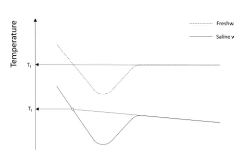
below the freezing temperature until it reaches the residual temperature. In saline water, the supercooling curves follows a slightly different pattern when compared to freshwater, as illustrated in the lower plot in Fig. 2. The shape of the curve and the physics of the process are the same as in freshwater up until the time the residual temperature is reached. In saline water during the residual phase of the supercooling curve, ice continues to form, causing the salinity of the water to contin-uously increase slowly. As a result, the residual temperature does not remain constant but decreases slowly (Brescia et al., 1975).
It was essential to determine the freezing point of water at the different salinities tested in these experiments. For this purpose, experiments were conducted to measure the freez-ing point at the three salinities and it was assumed to be 0◦C in freshwater. The experiment consisted of sampling approx-imately 1000 mL of water from the tank during each experi-ment at a given salinity. This water sample was then placed in the cold room during the experimental run and mixed us-ing a magnetic mixer. The water temperature in the stirred beaker was recorded using an RBR Solo temperature sen-sor. Supercooling curves for each of the freezing point de-pression experiments were plotted, and the linearly sloping portion of the residual was extrapolated back to where it
in-Figure 2.Typical supercooling curves showing the difference be-tween the freezing point temperatureTfin freshwater and saline water in a confined vessel. Adapted from She et al. (2016).
were−0.89±0.02,−1.48±0.02 and−2.09±0.02◦C, re-spectively.
4 Repeatability of experiments
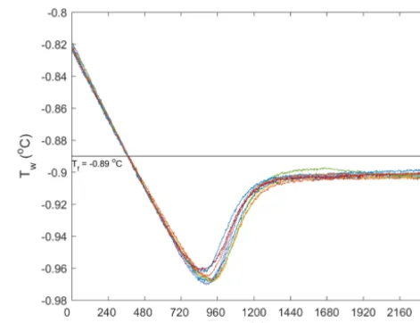
Repeated runs of experiments were conducted during each of the five series of experiments in order to reduce the un-certainty in the results by ensemble-averaging. In total, 62 experiments were conducted. Anomalous (i.e. outlier) runs (typically due to inconsistent air temperatures in the cold room, images out of focus, or frost build-up on the tank glass) were discarded from the analysis. This process eliminated 16 experiments and there were 9 to 10 repeated experiments that could be ensemble-averaged for each series of experiments. In Fig. 3, temperature time series from the 9 repeated runs conducted at a salinity of 15 ‰ are plotted. The supercool-ing curves aligned quite well, indicatsupercool-ing that the experimen-tal conditions in the cold room were adequately controlled and produced repeatable experiments. Note that a negative slope was not observed during the residual of the freezing point depression experiments in saline water, as was illus-trated in Fig. 2. This was because the quantity of ice pro-duced in the tank relative to the total volume of water in the tank was not large enough to reduce the freezing point significantly. A summary of the statistics of the temperature time series during the five series of experiments is presented in Table 2. The maximum supercooling, defined as the min-imum temperature minus the freezing point, and the cool-ing rates ranged between−0.075 and−0.092◦C and 0.009 and 0.012◦C min−1, respectively. The coefficient of varia-tion (standard deviavaria-tion divided by the arithmetic mean) of the maximum supercooling and the cooling rates ranged be-tween 2 % and 5 % and bebe-tween 3 % and 7 %, respectively, confirming the experiments were repeatable within accept-able limits.
5 Data processing 5.1 Raw images
The raw images of the frazil ice particles and flocs from each experiment were visually examined to assess the qualitative characteristics of the freshwater and saline water frazil ice particles. This visual analysis helped guide the development of the image processing algorithm used to compute the prop-erties of frazil ice particles and flocs. In Fig. 4, a pair of rep-resentative raw images a salinity of 35 ‰ and in freshwa-ter are shown to illustrate the qualitative differences between frazil ice particles and flocs in saline water and freshwater. An image at salinity of 35 ‰ is presented but the qualita-tive characteristics of the particles and flocs at this salinity are similar to those observed at salinities of 15 ‰ and 25 ‰. Figure 5 presents a zoomed view of the different particles’ shapes observed in the experiments. In freshwater
experi-Figure 3.Superimposed supercooling curves from repeated exper-iments showing water temperature,Tw(◦C), as a function of time, t(s), for a salinity of 15 ‰. The different curves represent repeated experiments, and the freezing temperatureTf (◦C) is indicated by the horizontal line.
ments, the typical shape of the particles was very consistent with previously reported studies, in that the individual frazil ice particles were predominantly disc-shaped. In saline wa-ter experiments, the shapes of individual frazil ice particles were a combination of disc, dendritic, hexagonal and other irregular shapes as shown in Fig. 5.
The average size of frazil particles appeared to be larger in freshwater than in saline water experiments. Also, in fresh-water frazil ice flocs were remarkably bigger than those in saline water and tended to rise to the surface even when the turbulence created from the propellers was still present, while in saline water flocs remained in suspension until the propellers were turned off. In saline water, there are many smaller flocs, comprised largely of irregularly shaped parti-cles. In stark contrast, in the freshwater image (Fig. 4b), there are fewer smaller flocs present and one very large floc that dominated the image. The very large freshwater floc is an or-der of magnitude larger than the largest floc visible in saline water image, and it is evident that freshwater flocs are com-prised largely of disc-shaped particles. There were no sig-nificant differences observed when visually comparing the particles and flocs sizes at non-zero salinities.
5.2 Image processing
Figure 4. Raw digital images showing frazil particles and flocs for(a)35 ‰ and(b)freshwater. Image dimensions are 3.07 cm by 4.61 cm.
(collected before frazil ice production starts) were subtracted from each image in the series. The raw images from the series were then converted to grayscale by eliminating the hue and saturation information while retaining the luminance. The grayscale images were then converted to a binary image us-ing a simple threshold. The threshold value is specified as a scalar luminance value between 0 and 1. As such any pixel with a scalar luminance value less than the specified thresh-old would be assigned a value of 0 (black) and any pixel with a scalar luminance value greater than the specified threshold would be assigned a value of 1 (white). At this point in the algorithm, the white objects correspond to frazil ice particles and/or flocs and the black pixels correspond to the dark ice-free background. Any objects that were touching the border of the image were eliminated from the binary image to pre-vent properties of portions of individual frazil ice particles and flocs from being computed. Finally, the white objects in the binary images were then dilated and eroded by five pixels to smooth and fill any insignificant holes smaller than five pixels that were generated due to the thresholding of the images. Next, the objects that represent individual frazil ice particles or flocs were analysed for key properties such as the
area, perimeter and the centroid. In addition, the major and minor axis lengths and eccentricity of a fitted ellipse that has the same second moments as the detected object were also computed. The eccentricity,e, of an ellipse is calculated as follows:
e= s
1−b 2
a2, (1)
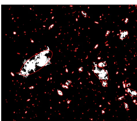
wherea andb are semi-major and semi-minor axis length of the fitted ellipse of a given particle or floc, respectively. Ellipses have eccentricity between zero and one, where an eccentricity of zero corresponds to a circle and an eccentric-ity of one corresponds to a straight line. Figure 6 presents a binary image with superimposed fitted ellipses over detected frazil particles or flocs. It can be seen in Fig. 6 that the ma-jor axes of the ellipses do provide an accurate estimate of ice particle and floc sizes. Therefore, the major axis length of the fitted ellipse is reported as the size of the frazil ice par-ticles and flocs throughout the analysis following Clark and Doering (2009).
Figure 5.Different kinds of shaped particles observed in the experiments:(a)disc-shaped,(b)dendritic,(c)hexagonal and(d)irregular.
Figure 6.Binary image with superimposed fitted ellipses plotted over each detected particle or floc.
that a threshold ratio of 1.1 correctly categorized the objects 95 % of the time. That is, if the ratio of an object’s area-over-perimeter to its fitted ellipse’s area-over-area-over-perimeter is greater than 1.1, then the object was identified as a frazil ice floc. Another benefit of using the properties of a fitted ellipse is that it provides information about the volume of ice particles or flocs from the volume of a fitted ellipsoid,V, calculated as follows:
V =4
3π abc, (2)
wherecis the dimension perpendicular to the plane of the image which is unknown. To estimate floc volume, it was assumed thatcwas equal to the average of aandbbut not greater than the distance between the polarizers when using Eq. (2). Based on the results of the experiments, the com-puted average eccentricity was ∼0.82, which translates to
b≈0.6a. Assumingcto be the average ofaandbresults in a mean volume equal to 4/3π (0.48a3). In the two extreme cases when cis equal to eithera or b (the major or minor axes), the volume would range between 4/3π (0.60a3) and
4/3π(0.36a3), respectively. Therefore, an approximate esti-mate of the error in computing floc volume would be±25 %. Ifcis less thanbor greater thana then the error would in-crease and this likely does occur in extreme cases, but we think the vast majority of flocs fall within these limits. When estimating the volume of an individual particle, it was as-sumed that the particles are approximately disc-shaped and that the diameter to thickness aspect ratio of the individual particles was equal to 37, which was the mean aspect ratio obtained by McFarlane et al. (2014). In all salinities, it was found that the total volume of frazil ice particles was between 0.3 % and 1 % of the total volume of flocs. Therefore, the vol-ume of frazil ice particles was neglected when computing ice volumes.
6 Data analysis
Figure 7.Typical water supercooling curve as a function of time, wheretfis the time of freezing,tmis the time of minimum temper-ature,tcis the time of cooling andTfis the freezing temperature.
therefore the experiment was considered finished at this point in time.
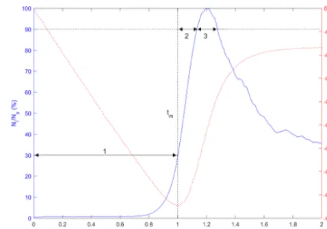
Three time phases were defined to assist in comparing re-sults at different times in the supercooling process for both particles and flocs as illustrated in Fig. 8. Phase 1 is defined as the time from when the water reached the freezing tem-perature (t /tc=0) to the time when the water reached the maximum supercooling temperature (t /tc=1.0). The other two phases were defined relative to when the peak number of particles or flocs were observed in the ensemble-averaged time series following Clark and Doering (2006). Phase 2 is defined as the time from t /tc=1.0 to the time when 90 % of the peak number of particles or flocs is reached (t90a).
Phase 3 is defined as the time from t90a to the time when
90 % of the peak number of particles or flocs is reached on the other side of the peak (t90b). These three phases were well
defined for individual particle experiments at all four salin-ities and for the freshwater floc experiments. For the saline water floc experiments, the number of flocs reached a peak and then remained at a value above 90 % of the peak for the remainder of the time interval, and therefore t90b does not
exist in this case. To consistently compare the results from the freshwater and saline water floc experiment, the Phase 3 dimensionless time interval from the freshwater floc exper-iments was used to estimate the results for Phase 3 for the saline water floc experiments.
The volume of flocs estimated from the image process-ing algorithm was used to estimate the volume concentra-tion of ice produced at the end of the principal supercooling. The volume of the fitted ellipsoid was multiplied by a fac-tor that accounts for the porosity of the ice. Ghobrial (2012) conducted slush layer experiments in the same tank and esti-mated the slush porosity to be between 0.80 and 0.85. Also, Beltaos (2013) suggested a porosity of 0.80 may be a rea-sonable estimate. Therefore, the volume of ice contained in a floc was estimated by multiplying the volume of its fitted el-lipsoid by 0.20. A set of 25 images starting at the end of the principal supercooling were analysed to get an average ice volume at this point in time for each experiment. The
vol-Figure 8.Typical plot illustrating the three time phases (labelled as 1, 2 and 3) with the dimensionless number of particles or flocs per image (in blue) plotted as a function of dimensionless time with a superimposed supercooling curve (in red).Niis the number of particles or flocs per image,Npis the peak number of particles or flocs per image,Twis the water temperature (◦C),tis the time (s),tc is the time of cooling (s) andtmis the time of minimum temperature (s). Note that this plot was generated from a freshwater experiment where the freezing temperatureTfis 0◦C.
ume of the field of view was then calculated based on the determined pixel sizes and space between the polarizers for each set-up (see Table 1). The frazil ice volume concentra-tion was estimated by computing the ratio of the volume of ice to the volume of the field of view. Finally, the shape of a floc (i.e. more elongated or more circular) was quantified by computing the eccentricity of its fitted ellipse.
7 Results 7.1 Time series
Figures 9 and 10 present an example of the synchronized time series generated for the frazil particles and flocs, re-spectively, for the 15 ‰ set of experiments. In these figures, particle and floc concentrations are calculated in terms of the number (N) of particles/flocs per unit volume (cm3). Al-though only time series of the 15 ‰ experiments are shown, the trends in all experiments were similar, in that the time series from all experiments line up together very well, con-firming the repeatability of the experiments. The time se-ries from the different experiments at each salinity were then ensemble-averaged for particles and flocs, as shown in Figs. 11 and 12.
de-Figure 9.Time series of frazil ice particle properties for all 15 ‰ experiments (shown in different colours).(a)Ni, the number of frazil ice particle per unit volume (cm−3),;(b)µi, the mean size of frazil ice particles (mm); and(c)σi, the standard deviation of the size of frazil ice particles (mm). Note that the data were smoothed using a 35 s moving average.
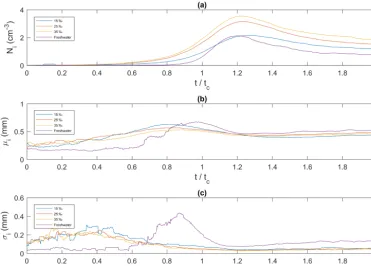
Figure 11.Ensemble-averaged time series of frazil ice particle properties for all four salinities plotted as a function of dimensionless time. (a)Ni, the average frazil ice particle concentration (cm−3);(b)µi, the mean size of frazil ice particles (mm); and(c)σi, the standard deviation of the size of frazil ice particles (mm).t /tc=1 corresponds to the time of the minimum temperature on the supercooling curves.
creased and then asymptotically approached a constant value. In freshwater the peak particle concentration was 2.1 cm−3 at t /tc=1.20, and in saline water the peaks were 2.2, 3.2, and 3.6 cm−3att /tc=1.28, 1.24, and 1.23 at 15 ‰, 25 ‰, and 35 ‰, respectively. The 35 ‰ curve had the highest par-ticle concentration throughout the entire time interval, and the freshwater curves had the lowest particle concentration throughout nearly the entire time interval, except near its peak where the freshwater concentration was briefly greater than the 15 ‰ concentration. In Fig. 11b the mean individ-ual frazil ice particle size initially increased, reached a peak, decreased and then reached an asymptotic value of approxi-mately 0.5 mm in all four cases. The average growth rate of frazil particle was estimated for the initial growth period and was found to be 0.174, 0.070, 0.033 and 0.024 mm min−1 for 0 ‰, 15 ‰, 25 ‰ and 35 ‰, respectively. The maximum mean particle size for the three higher salinities occurred prior to when the maximum size was reached in freshwa-ter. The maximum mean particle size occurred att /tc=0.96, 0.81, 0.79 and 0.88 for 0 ‰, 15 ‰, 25 ‰ and 35 ‰, respec-tively. The maximum mean size in freshwater was the largest at 0.68 mm, followed by 0.63, 0.57 and 0.53 mm for 15 ‰, 25 ‰ and 35 ‰, respectively. Figure 11c shows that the time series of the standard deviation are very similar in saline wa-ter, where it increased from approximately 0.1 to 0.2 mm and reached a constant value of approximately 0.04 mm at
ap-proximately t /tc=1 until the end of the experiment. The standard deviation in freshwater was initially constant at a value of∼0.05 mm, then att /tc=0.6 it started to increase and reached a peak value of∼0.45 mm att /tc=0.87. Af-ter that it decreased quickly to a minimum att /tc=1.23 and then slowly increased.
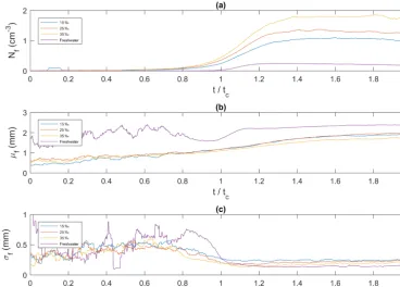
In Fig. 12a, the times series of frazil ice floc concentra-tion, defined as the number of flocs per unit volume (cm3), has a similar shape in the saline water experiments. The floc concentration increased from zero initially, reached a maximum value and then remained approximately constant until the end of the experiments. In freshwater, the trend was slightly different, with the floc concentration reaching a maximum value of 0.25 cm−3att /t
Figure 12.Ensemble-averaged time series of floc properties for all four salinities plotted as a function of dimensionless time.(a)Nf, the average floc concentration (cm−3)(b)µf, the mean size of flocs (mm) and(c)σf, the standard deviation of the size of flocs (mm).t /tc=1 corresponds to the time of the minimum temperature on the supercooling curves.
t /tc∼1.13 and continued increasing very slowly to 2.40 mm until t /tc=2.0. In saline water the mean floc size varied slightly with salinity and was always smaller than the fresh-water floc sizes. In general, the mean floc size in saline fresh-water increased from ∼0.5 mm at the start of the experiments up to∼1.90 mm at the end. The average floc growth rate was 0.408, 0.118, 0.089 and 0.072 mm min−1for the 0 ‰, 15 ‰, 25 ‰ and 35 ‰, respectively. Figure 12c shows that the time series of the standard deviation of floc size att /tc≤1.0 were quite noisy due to the small floc concentration. Att /tc≥1.0 the standard deviation curves in all cases was approximately constant and varied between ∼0.15 to∼0.25 mm with the lowest value being in freshwater.
7.2 Size and volume distributions
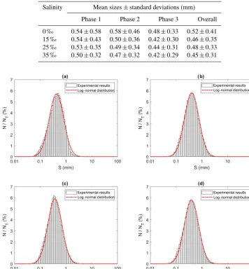
Figures 13 to 15 present the plots of the size distributions of frazil particles and flocs and volume distributions of flocs, re-spectively, for the 35 ‰ experiments during the three phases and the overall average (i.e. averaged over the entire du-ration). Although only distributions from the 35 ‰ experi-ments are presented, plots at the other salinities were very similar. It can be seen in Fig. 13 that the particles’ size dis-tributions during the three phases and the overall average closely follow a log-normal distribution. The log-normal dis-tribution is defined by the mean and standard deviation of the logarithmic of the variable (i.e. size or volume of particles or
flocs). The arithmetic mean and the corresponding standard deviation of particles sizes at all salinities are presented in Table 3. The mean size of frazil ice particles averaged over the entire duration (0≤t /tc≤2), defined as the overall mean size, were 0.52, 0.46, 0.48 and 0.45 mm for salinities of 0 ‰, 15 ‰, 25 ‰ and 35 ‰, respectively. The overall mean par-ticle size in freshwater was 8.3 % to 15.6 % larger than in saline water. The standard deviation decreased as salinity in-creased in all phases and overall. In addition, the standard deviation decreased with time for all salinities (from Phase 1 to Phase 3), with the largest decreases observed in the fresh-water and the smallest decrease observed at 35 ‰. The data in Table 3 show that in saline water the maximum mean par-ticle size occurred during Phase 1 and decreased during the latter two phases 2 and 3. Conversely, for the freshwater ex-periments, the maximum mean particle size occurred during Phase 2.
in-Table 3.Arithmetic mean sizes and corresponding standard deviations of frazil ice particles during different phases at all four salinities.
Salinity Mean sizes±standard deviations (mm)
Phase 1 Phase 2 Phase 3 Overall
0 ‰ 0.54±0.58 0.58±0.46 0.48±0.33 0.52±0.41 15 ‰ 0.54±0.43 0.50±0.36 0.42±0.30 0.46±0.35 25 ‰ 0.53±0.35 0.49±0.34 0.44±0.31 0.48±0.33 35 ‰ 0.50±0.32 0.47±0.32 0.42±0.29 0.45±0.31
Figure 13.Size distributions of individual particles at a salinity of 35 ‰ during(a)Phase 1,(b)Phase 2,(c)Phase 3 and(d)the entire time interval (i.e. averaged over all three phases).N is the number of particles in each bin,NTis the total number of particles (NT≈13 620, 22 430, 105 560 and 141 610 ina,b,candd, respectively), andSis the particle size (mm). Note that the arithmetic mean of particles sizes were 0.50, 0.47, 0.42 and 0.45 mm for(a),(b),(c)and(d), respectively.
creased from 15 ‰ to 35 ‰. The standard deviation of floc sizes in freshwater was significantly larger than in saline wa-ter and it decreased as salinity increased. At all four salinities, as the experiment progressed the mean size and standard de-viation of the flocs increased and reached its maximum dur-ing Phase 3 of the experiment.
As discussed previously it was observed that there were very large flocs present in the freshwater experiments that were not observed in the saline water experiments. In order to assess this observation quantitatively, the 95th percentile of floc sizes, the maximum floc size and the mean size of flocs larger than the 95th percentile were computed, and these re-sults are listed in Table 5. The 95th percentile of floc size was 6.91 mm in freshwater and decreased with increasing
salin-ity to 3.96 mm at 35 ‰. The mean size of the largest 5 % of flocs varied from 11.9 mm in freshwater and decreased with increasing salinity to 5.38 mm at 35 ‰. The maximum floc size in freshwater was 95 mm, compared to 23 to 36 mm in the saline water cases. The data in Table 5 support the qual-itative observation that the flocs were considerably larger in freshwater and that floc size decreased slightly as the salinity increased from 15 ‰ to 35 ‰.
Table 4.Arithmetic mean sizes and corresponding standard deviations of frazil ice flocs during different phases at all four salinities.
Salinity Mean sizes±standard deviations (mm)
Phase 1 Phase 2 Phase 3 Overall
0 ‰ 1.68±1.19 2.28±2.06 2.65±3.09 2.57±2.88 15 ‰ 0.93±0.96 1.45±1.30 1.83±1.81 1.64±1.63 25 ‰ 1.02±0.81 1.39±1.09 1.77±1.57 1.61±1.43 35 ‰ 0.96±0.82 1.30±1.01 1.60±1.40 1.47±1.28
Figure 14.Size distributions of flocs at a salinity of 35 ‰ during(a)Phase 1,(b)Phase 2,(c)Phase 3 and(d)the entire time interval (i.e. averaged over all three phases).N is the number of flocs in each bin,NTis the total number of flocs (NT≈23 880, 136 950, 270 790 and 431 620 ina,b,candd, respectively) andSis the floc size (mm). Note that the arithmetic mean of flocs sizes were 0.96, 1.30, 1.60 and 1.47 mm for(a),(b),(c)and(d), respectively.
35 ‰, respectively. This equates to the average floc volume being 8 to 15 times greater in freshwater than in saline water. 7.3 Floc porosity and eccentricity
The volume concentration of ice at the end of the principal supercooling in 0 ‰, 15 ‰, 25 ‰ and 35 ‰ was estimated to be 0.0028, 0.0031, 0.0028 and 0.0021 m3m−3, respectively. These volume concentrations can be compared to the theo-retical values calculated by considering the thermodynamic conditions of the experiment assuming the tank is fully mixed (Osterkamp, 1978; Ye et al., 2004). The total heat exchanged with the surrounding environment,Qtw in W m−3, is given by
Qtw=ρCp
dT
dt , (3)
whereρis the density of water in kg m−3,Cpis the specific
heat of the water in J (kg◦C)−1and dT /dtis the cooling rate in◦C s−1. Density and specific heat depend on salinity and were calculated following Gill (1982). The cooling rate was obtained by calculating the slope of the supercooling curve over an interval beginning 15 min prior to freezing and end-ing at the freezend-ing point. The volume concentration of frazil ice,Mspin m3m−3, is then given by
Msp=
Qtwtsp
Liρi
, (4)
Table 5.Sizes of the largest frazil ice flocs at all four salinities.
Salinity 95th percentile Mean size of flocs larger than Maximum floc size
(mm) 95th percentile (mm) (mm)
0 ‰ 6.91 11.89 95.10
15 ‰ 4.82 6.77 36.22
25 ‰ 4.38 5.98 23.18
35 ‰ 3.96 5.38 25.19
Table 6.Estimated arithmetic mean volumes and corresponding standard deviations of frazil ice flocs during different phases at all four salinities.
Salinity Mean volumes±standard deviations (mm3)
Phase 1 Phase 2 Phase 3 Overall
0 ‰ 0.40±1.07 3.01±37.68 10.67±141.45 8.79±117.98 15 ‰ 0.21±4.70 0.60±4.36 1.54±7.78 1.14±6.68 25 ‰ 0.15±0.71 0.39±1.49 1.08±4.55 0.82±3.78 35 ‰ 0.16±2.62 0.31±1.05 0.78±3.22 0.60±2.72
the computed volume concentrations of ice formed during the principal supercooling were 0.0019, 0.0027, 0.0028 and 0.0027 m3m−3for 0 ‰, 15 ‰, 25 ‰ and 35 ‰, respectively. This information was also used to estimate the porosity of frazil flocs, by equating the theoretical volume concentration of ice computed thermodynamically using Eq. (4) to the es-timated total floc volume computed from the images. This calculation gave estimated porosities for frazil ice flocs of 0.86, 0.82, 0.80 and 0.75 for 0 ‰, 15 ‰, 25 ‰ and 35 ‰, respectively.
The mean eccentricity of frazil flocs was 0.84, 0.82, 0.81 and 0.81, which corresponds to ratios of major to minor axis length of 1.84, 1.75, 1.71 and 1.71 for 0 ‰, 15 ‰, 25 ‰ and 35 ‰, respectively. These eccentricity values indicate that the average shape of flocs in saline water did not vary signif-icantly and that the average shape of flocs was slightly more elongated in freshwater compared to saline water.
8 Discussion
The ensemble-averaged time series of frazil ice particle con-centration showed that, in general, the higher the salinity, the higher the particle concentration (Fig. 11a). As the salt is re-jected by the ice, this can create a small pocket around the ice particle with a higher salinity and slightly lower freezing point (Rees Jones and Wells, 2015), thus inhibiting the floc-culation process. This would result in fewer particles adher-ing and sinteradher-ing together to form flocs, leavadher-ing more parti-cles in suspension and producing the observed result of more individual particles being present at higher salinities. All of the time series of the particle concentration follow a simi-lar pattern of initially increasing, reaching a maximum and then decreasing with time. This pattern can be explained by
considering particle production and the flocculation process. The flocculation rate, defined as the rate at which particles are sintered to other particles or flocs, is a function of the particle concentration. This is because when there are more particles there is higher likelihood of particle to particle and particle to floc collisions, which present opportunities for sin-tering. Prior to the time when the peaks occur in the time series, particle production exceeds the flocculation rate, but as time progresses a point is reached where particle produc-tion equals the rate of flocculaproduc-tion and the peak occurs at this time. This balance is reached because the flocculation rate is increasing as can be seen in the time series plots of flocs concentration in Fig. 12a. As time progresses both the parti-cle production and the rate of flocculation reach asymptotic values when the water is at the residual temperature.
Figure 15.Size distributions of floc volume at a salinity of 35 ‰ during(a)Phase 1,(b)Phase 2,(c)Phase 3 and(d)the entire time interval (i.e. average over all three phases).Nis the number of flocs in each bin,NTis the total number of flocs (NT≈23 880, 136 950, 270 790 and 431 620 ina,b,candd, respectively) and V is the estimated floc volume (mm3). Note that the arithmetic mean of flocs volumes were 0.16, 0.31, 0.78 and 0.60 mm3for(a),(b),(c)and(d), respectively.
Phase 1 and reach their maximum mean size later in the pro-cess during Phase 2.
The time series plots in Fig. 12a showed that throughout an entire experiment the higher the salinity, the higher the floc concentration. As salinity increases, the strength of par-ticle to parpar-ticle bonds decreases, and therefore flocs remain smaller in size. This is because as flocs grow larger the shear forces that cause them to rupture also increase, and there-fore weaker internal bonds leads to smaller flocs and higher floc concentrations (Hanley and Tsang, 1984). Eventually, at t /tc≈1.4, the floc concentration curves reach a plateau which suggests that particle to floc sintering becomes the dominant process as this process produces a net zero con-tribution to floc concentration. This is logical because at this point the particle production rate has decreased, resulting in low particle concentrations, which reduces the probability of two particles colliding to near zero. However, the concen-tration of flocs is high, making particle floc collisions much more probable. Note that, in freshwater, floc concentration increased, reached a peak and then slowly decreased starting fromt /tc≈1.2. This can be explained by the visual obser-vation that flocs in freshwater tended to rise to the surface before the experiment was completed, whereas saline water flocs tended to remain suspended until the end of the experi-ment. The larger mean size of freshwater flocs increases their
buoyancy, and thus increases their ability to overcome the turbulence of the flow and rise to the surface. This result is similar to observations made by Kempema et al. (1993).
The mean floc size increased as the experiments pro-gressed (Fig. 12b) indicating that the mean volume of flocs also increased. As particle production continues, the prob-ability of collisions of particles to flocs increases, resulting in a continuous increase in the mean floc size, especially in saline water. Later in the process, when the particle produc-tion slows down, most of the collisions would be particle to floc, resulting in the slow steady growth of flocs until the end of the time of the experiments. In freshwater, the rapid increase in floc sizes started att /tc≈1 with a rate that was 4 times faster than in the saline water but over a much shorter time interval.
1993; Smedsrud, 2001). However, these previously reported estimates of size ranges were based on very small sample sizes and used less sophisticated measuring techniques, in-cluding visual observations, which may have influenced the results. The overall mean size of particles in freshwater was on average 1.13 times larger than in saline water. This sug-gests that the nucleation and growth of frazil ice particles are fairly similar in fresh and saline water. The particle size dis-tributions at all salinities were log-normal, which is further evidence that the processes involved are similar.
The overall mean size of flocs in freshwater was signifi-cantly larger than in saline water. Past studies have reported similar qualitative results that freshwater flocs are larger and more adhesive than saline water flocs (Hanley and Tsang, 1984; Kempema et al., 1993). The overall mean size of flocs in freshwater was 2.57 mm, which suggests that Clark and Doering (2009) criterion of defining a floc as any particle larger than 17 mm did not capture the full spectrum of the floc size distribution. Flocs in freshwater were on average 1.64 times larger than in saline water. The maximum floc size observed in the freshwater experiments was approximately 3 times larger than in the saline water experiments. The dif-ference in the flocculation process can be explained by freez-ing point depression in saline water. As the salt is rejected by the ice, it will increase the salinity of the surrounding water and slightly reduce the freezing point. This will inhibit the process of adhering and sintering, thus resulting in the mean size of flocs decreasing with salinity.
The overall mean volume of flocs in freshwater was on average approximately 10 times larger than in saline water. It is interesting to note that there is large difference between the floc sizes when comparing freshwater to saline water, but the variation in saline water is less significant. This is further evidence that the flocculation process is largely dependent on whether the process occurs in saline water or freshwater and less dependent on precise value of the salinity.
The volume concentrations estimated from the image pro-cessing are very close to the theoretical values computed thermodynamically. This indicates that assuming flocs are el-lipsoid and have a porosity of 80 % may provide a reasonable estimate of the ice volume concentration contained in flocs. Also, the deduced floc porosities decreased with decreasing salinities from 0.86 for freshwater to 0.75 at the highest salin-ity. These values are within the range of previously reported freshwater slush porosities (Beltaos, 2013; Ghobrial, 2012) and the porosity of the sub-ice platelet layer in the polar re-gions (Langhorne et al., 2015).
9 Conclusions
A total of 46 laboratory experiments were performed to de-termine the properties of individual frazil ice particles and flocs at salinities of 0 ‰, 15 ‰, 25 ‰ and 35 ‰. Visual ex-amination of the images clearly showed that there were more
irregularly shaped particles in saline water than in freshwater. The average particle and floc growth rates decreased as salin-ity increased and the freshwater growth rates were approxi-mately 4 times larger than the average growth rate in saline water. The mean frazil ice particle sizes ranged between 0.52 and 0.45 mm with particles sizes in freshwater∼13 % larger than in saline water. This indicates that mean particle sizes are only weakly dependent on salinity. The mean floc sizes ranged between 2.57 and 1.47 mm for freshwater and saline water with freshwater flocs being on average 60 % larger than in saline water. A log-normal distribution was observed to fit all the particle and flocs size distributions closely. The esti-mated floc porosities were equal to 0.86, 0.82, 0.80 and 0.75 for salinities of 0 ‰, 15 ‰, 25 ‰, 35 ‰, respectively, which suggests that as salinity increases porosity decreases.
Data availability. Data are available from the authors upon request.
Author contributions. CCS and MRL designed the experiments and CCS carried them out and prepared the figures and first draft. TRG prepared the paper, including the analysis and discussion with re-view and contributions from MRL.
Competing interests. The authors declare that they have no conflict of interest.
Acknowledgements. We would like to thank the Natural Sciences and Engineering Research Council of Canada (NSERC) for sup-porting this project (RGPIN-2015-04670 and RGPAS 477890-2015) and Perry Fedun for his valuable technical assistance. We are grateful for that support.
Financial support. This research has been supported by the Natural Sciences and Engineering Research Council of Canada (NSERC) (grant nos. RGPIN-2015-04670 and RGPAS 477890-2015).
Review statement. This paper was edited by John Yackel and re-viewed by three anonymous referees.
References
Banner, M. L. and Morison, R. P.: On the upper ocean turbulent dissipation rate due to microscale break-ers and small whitecaps, Ocean Model., 126, 63–76, https://doi.org/10.1016/j.ocemod.2018.04.004, 2018.
Beltaos, S.: River Ice Formation, 1st Edn., Committee on River Ice Processes and the Environment, Edmonton, AB, 2013.
Brescia, F., Arents, J., Herbert, M., Turk, A., and Weiner, E.: Funda-mentals of Chemistry: Laboratory Studies, 3rd Edn., Academic Press, Inc., New York, 1975.
Cavalieri, D. J. and Martin, S.: The contribution of Alaskan, Siberian, and Canadian coastal polynyas to the cold halocline layer of the Arctic Ocean, J. Geophys. Res., 99, 18343–18362, 1994.
Chanona, M., Waterman, S., and Gratton, Y.: Variability of internal wave-driven mixing and stratification in Canadian Arctic shelf and shelf-slope waters, J. Geophys. Res.-Oceans, 123, 9178– 9195, https://doi.org/10.1029/2018JC014342, 2018.
Clark, S. and Doering, J.: Laboratory Experiments on Frazil-Size Characteristics in a Counterrotating Flume, J. Hy-draul. Eng., 132, 94–101, https://doi.org/10.1061/(ASCE)0733-9429(2006)132:1(94), 2006.
Clark, S. P. and Doering, J. C.: Frazil flocculation and secondary nucleation in a counter-rotating flume, Cold Reg. Sci. Technol., 55, 221–229, https://doi.org/10.1016/j.coldregions.2008.04.002, 2009.
Daly, S.: Report on frazil ice, US Army Corp of Engineers, Cold Regions Research & Engineering Laboratory, Report 94-23, Hanover, New Hampshire, 50 pp., 1994.
Daly, S. F. and Colbeck, S.: Frazil Ice Measurements in CRREL’s Flume Facility, Proc. Syrup. Ice, Int. Assoc. Hydraul. Res., Iowa City, Iowa, 427–438, 1986.
De Santi, F. and Olla, P.: Limit regimes of ice formation in turbulent supercooled water, Phys. Rev. E, 96, 043106, https://doi.org/10.1103/PhysRevE.96.043106, 2017.
Galton-Fenzi, B. K., Hunter, J. R., Coleman, R., Marsland, S. J., and Warner, R. C.: Modeling the basal melting and marine ice accretion of the Amery Ice Shelf, J. Geophys. Res., 117, 1–19, https://doi.org/10.1029/2012JC008214, 2012.
Ghobrial, T. R.: Characterization of suspended frazil and surface ice in rivers using sonars, PhD thesis, University of Alberta, 2012. Ghobrial, T. R., Loewen, M. R., and Hicks, F. E.: Laboratory
calibration of upward looking sonars for measuring suspended frazil ice concentration, Cold Reg. Sci. Technol., 70, 19–31, https://doi.org/10.1016/j.coldregions.2011.08.010, 2012. Ghobrial, T. R., Loewen, M. R., and Hicks, F. E.:
Char-acterizing suspended frazil ice in rivers using upward looking sonars, Cold Reg. Sci. Technol., 86, 113–126, https://doi.org/10.1016/j.coldregions.2012.10.002, 2013. Gill, A. E.: Atmosphere-Ocean Dynamics, Academic Press, Inc.,
San Diego, California, 1982.
Gosink, J. P. and Osterkamp, T. E.: Measurements and analysis of velocity profiles and frazil ice-crystal rise velocities, Ann. Glaciol., 4, 79–84, 1983.
Hanley, T. O. D. and Tsang, G.: Formation and properties of frazil in saline water, Cold Reg. Sci. Technol., 8, 209–221, https://doi.org/10.1016/0165-232X(84)90052-1, 1984.
Hicks, F. E.: An Overview of River Ice Problems, invited paper, Cold Reg. Sci. Technol., 55, 175–185, 2009.
Hobbs, P. V.: Ice Physics, Oxford University Press, New York City, 1970.
Holland, P. R., Feltham, D. L., and Daly, S. F.: On the Nusselt number for frazil ice growth – a correc-tion to “Frazil evolucorrec-tion in channels” by Lars Ham-mar and Hung-Tao Shen, J. Hydraul. Res., 45, 421–424, https://doi.org/10.1080/00221686.2007.9521775, 2007. Kempema, E. W., Reimnitz, E., Clayton, J. R. J., and Payne,
J. R.: Interactions of frazil and anchor ice with sedimentary particles in a flume, Cold Reg. Sci. Technol., 21, 137–149, https://doi.org/10.1016/0165-232X(93)90003-Q, 1993.
Langhorne, P. J., Hughes, K. G., Gough, A. J., Smith, I. J., Williams, M. J. M., Robinson, N. J., Stevens, C. L., Rack, W., Price, D., Leonard, G. H., Mahoney, A. R., Haas, C., and Haskell, T. G.: Observed platelet ice distributions in Antarctic sea ice: An in-dex for ocean-ice shelf heat flux, Geophys. Res. Lett., 42, 5442– 5451, https://doi.org/10.1002/2015GL064508, 2015.
Mair, B. J., Glasgow, A. R., and Rossini, F. D.: Determination of freezing points and amounts of impurity in hydrocarbons from freezing and melting curves, J. Res. Natl. Bur. Stand., 26, 591– 620, 1941.
Martin, S.: Frazil ice in rivers and oceans,
Annu. Rev. Fluid Mech., 13, 379–397,
https://doi.org/10.1146/annurev.fl.13.010181.002115, 1981. Martin, S. and Kauffman, P.: A field and laboratory study of wave
damping by grease ice, J. Glaciol., 27, 283–313, 1981.
McFarlane, V., Loewen, M., and Hicks, F. E.: Labora-tory measurements of the rise velocity of frazil ice particles, Cold Reg. Sci. Technol., 106–107, 120–130, https://doi.org/10.1016/j.coldregions.2014.06.009, 2014. McFarlane, V., Loewen, M., and Hicks, F. E.:
Mea-surements of the evolution of frazil ice particle size distributions, Cold Reg. Sci. Technol., 120, 45–55, https://doi.org/10.1016/j.coldregions.2015.09.001, 2015. McFarlane, V., Loewen, M., and Hicks, F. E.:
Measure-ments of the size distribution of frazil ice particles in three Alberta rivers, Cold Reg. Sci. Technol., 142, 100–117, https://doi.org/10.1016/j.coldregions.2017.08.001, 2017. Nihashi, S. and Ohshima, K. I.: Circumpolar Mapping of Antarctic
Coastal Polynyas and Landfast Sea Ice: Relationship and Vari-ability, J. Climate, 28, 3650–3669, https://doi.org/10.1175/JCLI-D-14-00369.1, 2015.
Ohshima, K. I., Nihashi, S., and Iwamoto, K.: Global view of sea-ice production in polynyas and its linkage to dense/bottom water formation, Geosci. Lett., 3, 13, https://doi.org/10.1186/s40562-016-0045-4, 2016.
Osterkamp, T. E.: Frazil Ice Formation: A Review, J. Hydr. Eng. Div.-ASCE, 104, 1239–1255, 1978.
Park, C. and Gerard, R.: Hydraulic characteristics of frazil flocs – some preliminary experiments, Proceeding of the IAHR Ice Symposium, Hamburg, Germany, 27–35, 1984.
Rees Jones, D. W. and Wells, A. J.: Solidification of a disk-shaped crystal from a weakly supercooled binary melt, Phys. Rev. E, 92, 022406, https://doi.org/10.1103/PhysRevE.92.022406, 2015. Rees Jones, D. W. and Wells, A. J.: Frazil-ice growth rate
and dynamics in mixed layers and sub-ice-shelf plumes, The Cryosphere, 12, 25–38, https://doi.org/10.5194/tc-12-25-2018, 2018.
Richard, M., Morse, B., Daly, F., and Emond, J.: Quan-tifying suspended frazil ice using multi-frequency under-water acoustic devices, River Res. Appl., 27, 1106–1117, https://doi.org/10.1002/rra.1446, 2011.
Scheifele, B., Waterman, S., Merckelbach, L., and Carpenter, J. R.: Measuring the dissipation rate of turbulent kinetic energy in strongly stratified, low-energy environments: A case study from the Arctic Ocean. J. Geophys. Res.-Oceans, 123, 5459–5480, https://doi.org/10.1029/2017JC013731, 2018.
She, Y., Kemp, J., Richards, L., and Loewen, M.: Investi-gation into freezing point depression in stormwater ponds caused by road salt, Cold Reg. Sci. Technol., 131, 53–64, https://doi.org/10.1016/j.coldregions.2016.09.003, 2016. Shen, H. T.: Mathematical modeling of river ice processes, Cold
Reg. Sci. Technol., 62, 3–13, 2010.
Skogseth, R., Nilsen, F., and Smedsrud, L. H.: Supercooled water in an Arctic polynya: Observations and modeling, J. Glaciol., 55, 43–52, https://doi.org/10.3189/002214309788608840, 2009. Smedsrud, L. H.: Frazil-ice entrainment of sediment:
Large-tank laboratory experiments, J. Glaciol., 47, 461–471, https://doi.org/10.3189/172756501781832142, 2001.
Smedsrud, L. H. and Jenkins, A.: Frazil ice formation in an ice shelf water plume, J. Geophys. Res., 109, 1–15, https://doi.org/10.1029/2003JC001851, 2004.
Svensson, U. and Omstedt, A.: Simulation of supercooling and size distribution in frazil ice dynamics, Cold Reg. Sci. Technol., 22, 221–233, https://doi.org/10.1016/0165-232X(94)90001-9, 1994. Tamura, T., Williams, G. D., Fraser, A. D., Ohshima, K. I.: Potential regime shift in decreased sea ice production after the Mertz Glacier calving, Nat. Commun., 3, 826, https://doi.org/10.1038/ncomms1820, 2012.
Ushio, S. and Wakatsuchi, M.: A laboratory study on su-percooling and frazil ice production processes in win-ter coastal polynyas, J. Geophys. Res., 98, 20321–20328, https://doi.org/10.1029/93JC01905, 1993.
Wang, B. and Liao, Q.: Field observations of turbulent dis-sipation rate profiles immediately below the air-water interface, J. Geophys. Res.-Oceans, 121, 4377–4391, https://doi.org/10.1002/2015JC011512, 2016.
Weeks, W. F.: On Sea Ice, 1st Edn., University of Alask Press, Fair-banks, Alaska, 2010.