https://doi.org/10.5194/tc-13-125-2019
© Author(s) 2019. This work is distributed under the Creative Commons Attribution 4.0 License.
New insight from CryoSat-2 sea ice thickness for sea ice modelling
David Schröder1, Danny L. Feltham1, Michel Tsamados2, Andy Ridout2, and Rachel Tilling3
1Centre for Polar Observation and Modelling, Department of Meteorology, University of Reading, Reading, RG6 6BB, UK 2Centre for Polar Observation and Modelling, Department of Earth Sciences,
University College London, London, WC1E 6BT, UK
3Centre for Polar Observation and Modelling, School of Earth and Environment, University of Leeds, Leeds, LS2 9JT, UK
Correspondence:David Schröder (d.schroeder@reading.ac.uk) Received: 3 August 2018 – Discussion started: 17 August 2018
Revised: 9 November 2018 – Accepted: 3 December 2018 – Published: 14 January 2019
Abstract. Estimates of Arctic sea ice thickness have been available from the CryoSat-2 (CS2) radar altimetry mission during ice growth seasons since 2010. We derive the sub-grid-scale ice thickness distribution (ITD) with respect to five ice thickness categories used in a sea ice component (Com-munity Ice CodE, CICE) of climate simulations. This allows us to initialize the ITD in stand-alone simulations with CICE and to verify the simulated cycle of ice thickness. We find that a default CICE simulation strongly underestimates ice thickness, despite reproducing the inter-annual variability of summer sea ice extent. We can identify the underestimation of winter ice growth as being responsible and show that in-creasing the ice conductive flux for lower temperatures (bub-bly brine scheme) and accounting for the loss of drifting snow results in the simulated sea ice growth being more real-istic. Sensitivity studies provide insight into the impact of ini-tial and atmospheric conditions and, thus, on the role of posi-tive and negaposi-tive feedback processes. During summer, atmo-spheric conditions are responsible for 50 % of September sea ice thickness variability through the positive sea ice and melt pond albedo feedback. However, atmospheric winter condi-tions have little impact on winter ice growth due to the domi-nating negative conductive feedback process: the thinner the ice and snow in autumn, the stronger the ice growth in winter. We conclude that the fate of Arctic summer sea ice is largely controlled by atmospheric conditions during the melting sea-son rather than by winter temperature. Our optimal model configuration does not only improve the simulated sea ice thickness, but also summer sea ice concentration, melt pond fraction, and length of the melt season. It is the first time CS2 sea ice thickness data have been applied successfully to im-prove sea ice model physics.
1 Introduction
Historical observations of sea ice thickness have been lim-ited due to their sparse spatial and temporal coverage of, and uncertainties in, measurements. Prior to the launch of the Eu-ropean Space Agency’s (ESA) first EuEu-ropean Remote Sens-ing satellite (ERS-1) in 1991, most data were collected from submarines operating beneath the Arctic pack ice. Upward-looking sonars measure the submerged portion of the ice (draft), which can be converted to thickness by making as-sumptions about the snow depth and the densities of ice, snow, and water. Based on sea ice draft observations from 34 US Navy submarines, a decrease of mean autumn sea ice thickness from 2.8 to 1.6 m could be identified over the pe-riod 1975–2000 within the central Arctic Ocean (Rothrock et al., 2008). While the accuracy and the spatial coverage were sufficient to give evidence of sea ice thinning in the Arctic and to provide a basis for simulating the trend, these data are of limited use for evaluating the spatial and temporal vari-ability of sea ice across the Arctic, and in climate models. More recently, cryosphere-focused satellite altimeters such as the NASA Ice, Cloud, and land Elevation Satellite (ICE-Sat) and ESA CryoSat-2 (CS2) have allowed estimation of sea ice thickness across the Arctic (Giles et al., 2007, 2008; Kwok and Rothrock, 2009; Laxon et al., 2013).
et al., 2018). PIOMAS is a reanalysis product, which does not include ice thickness observations. Stroeve et al. (2014) combined submarine, aircraft, and satellite data to evaluate sea ice thickness in climate model simulations. Their assess-ment revealed shortcomings regarding spatial patterns of sea ice thickness that were larger than uncertainties in the veri-fication data. CS2 sea ice thickness data have recently been used to initialize sea ice ocean and climate models to im-prove seasonal predictions (Allard et al., 2018; Blockley and Peterson, 2018).
In this study, we aim to improve sea ice physics and to calibrate poorly constrained parameters in the sea ice model CICE (Community Ice CodE) using the CS2 ice thickness data. Given that CS data are available from October to April, our focus lies on processes controlling winter ice growth. We note that several factors contribute to CS2-derived sea ice thickness uncertainties, including the assumption that the radar return is from the snow–ice interface (Willat et al., 2011), snow depth departures from climatology, and the use of fixed snow and ice densities. To enable a meaningful com-parison of sea ice thickness between CICE and CS2, we con-sider the strengths and weaknesses of the model and the data. We design experiments with perturbed physical parameteri-zations to close the gap between our default CICE simula-tion and CS2 as well as to investigate the impact of initial conditions and atmospheric forcing data. The latter experi-ments address questions regarding the impact of the last three exceptionally warm Arctic winters on the sea ice decline (Stroeve et al., 2018) and give new insight into the strengths of positive and negative feedback mechanisms that govern the evolution of sea ice.
2 Ice thickness distribution from CryoSat-2
The CS2 radar altimetry mission was launched in April 2010, providing estimates of ice thickness during the ice growth season from October to April. During summer the formation of melt ponds interferes with the radar signal, retarding accu-rate measurements. As for the derivation of sea ice thickness from the ice draft using submarine data, the freeboard (the height of sea ice above the water surface) is estimated from the satellite data and can be converted to thickness by as-suming hydrostatic equilibrium and applying values for the densities of ice, snow, and water as well as the snow depth. The principal challenges in deriving an accurate sea ice thick-ness using satellite altimetry are the discrimination of ice and open water, the discrimination of ice type, the retracking of radar waveforms to obtain height estimates, the construction of sea surface height beneath the ice, and estimation of the depth of the snow cover. Ice thickness is retrieved from the freeboard by processing CS2 Level 1B data, with a footprint of approximately 300 m×1700 m (Wingham et al., 2006), and assuming snow density and snow depth from the Warren et al. (1999) climatology (hereafter W99), modified for the
distribution of multi-year versus first-year ice (see Laxon et al., 2013, and Tilling et al., 2018, for data processing details). In this study, we bin the individual thickness point mea-surements provided by the Centre for Polar Observation and Modelling (CPOM) into five CICE thickness cate-gories, (1) ice thicknessh <0.6 m, (2) 0.6 m< h <1.4 m, (3) 1.4 m< h <2.4 m, (4) 2.4 m< h <3.6 m, and (5) h > 3.6 m, on a rectangular 50 km grid for each month. The mean area fraction and mean thickness are derived for each thick-ness category and these values are interpolated on the ORCA tripolar 1◦grid used by CICE (∼40 km grid resolution). Till-ing et al. (2018) derived a general grid cell ice thickness un-certainty of 25 %. Grid cells with fewer than 100 individ-ual measurements and a grid cell mean sea ice thickness of less than 0.5 m are omitted due to their increased uncertainty (Ricker et al., 2017). Otherwise, the whole range of indi-vidual observations from applied grid points are included. Negative thickness values are retained in the CS2 process-ing to prevent statistical positive bias of the thinner ice and are added to category 1. This approach allows us to initial-ize the CICE model with the full ice thickness distribution (ITD) rather than to derive the ITD from the mean sea ice thickness (Hunke et al., 2015). A realistic ITD is critical for simulating ice growth and ice melt rates correctly: given the identical mean ice thickness, a wider distribution leads to an increase of ice growth in winter because ice growth mainly takes place over the thinner ice, whereas during summer, the thinner ice melting away increases the lead fraction, resulting in a warmer ocean mixed-layer temperature, thus accelerat-ing the sea ice melt.
CS2 ice thickness data for October appear to be less robust as indicated by large differences between the three products for thin first-year ice (not shown) and by large differences in comparison with ESA’s Soil Moisture and Ocean Salinity (SMOS) sea ice data (Wang et al., 2016), so we only include CS data from November to April in our study.
3 Model set-up and simulations 3.1 Set-up
CICE is a dynamic–thermodynamic sea ice model designed for inclusion within a global climate model. The sea ice ve-locity is calculated from a momentum balance equation that accounts for air drag, ocean drag, Coriolis force, sea sur-face tilt, and the internal ice stress. The CICE model solves one-dimensional vertical heat balance equations for each ice thickness category. See Hunke et al. (2015) for a detailed description of the CICE model. Here, we perform stand-alone (fully forced) CICE simulations with version 5.1.2 for a pan-Arctic region (∼40 km grid resolution). CICE con-tains a simple mixed-layer ocean model with a prognos-tic ocean temperature. To account for heat transport in the ocean, we restore the mixed-layer ocean temperature and salinity to climatological monthly means from MYO-WP4-PUM-GLOBAL-REANALYSIS-PHYS-001-004 (Ferry et al., 2011) with a restoring timescale of 20 days. We apply a climatological ocean current (monthly means) from the same ocean reanalysis product. NCEP Reanalysis-2 (NCEP2) at-mospheric reanalysis data (Kanamitsu et al., 2002, updated 2017) are used as atmospheric forcing. We perform a multi-year simulation from 1980 to 2017 which does not utilize CS2 ice thickness data (referred to as CICE-free) and seven 1-year-long simulations which are initialized with CS2 ice thickness data (referred to as CICE-ini) starting in mid-November and running until the end of mid-November of the fol-lowing year for the seven winter periods from 2010/11 to 2016/17. The initial thickness and concentration for each of the five ice categories are taken from the CPOM CS2 ITD November mean thickness fields. For grid points without CS2 data, and for all other variables (e.g. temperature pro-files, snow volume), results from the free CICE simulation are applied. In this way, CICE simulations cover the pan-Arctic region, but in regions where no CS2 data are avail-able, we restart with ice thickness values from the free CICE model run. While this approach would be problematic in a coupled model, in a stand-alone sea ice simulation, the model adjustment to the new conditions is smooth and the impact of using the vertical temperature profile from the free simu-lation only affects sea ice thickness on the order of millime-tres.
3.2 Reference simulation (CICE-default)
Our reference simulation includes a prognostic melt pond model (Flocco et al., 2010, 2012) and the elastic anisotropic plastic rheology (Wilchinski and Feltham, 2006; Tsamados et al., 2013; Heorton et al., 2018). Otherwise, default CICE settings are chosen: seven vertical ice layers, one snow layer, linear remapping ITD approximation (Lipscomp and Hunke, 2004), Bitz and Libscomp (1999) thermodynamics, Maykut and Untersteiner (1971) conductivity, the Rothrock (1975) ridging scheme with a Cf value of 12 (empirical parameter that accounts for frictional energy dissipation), and the delta-Eddington radiation scheme (Briegleb and Light, 2007).
3.3 Simulations with perturbed physical
parameterizations and sensitivity simulations 3.3.1 Improving sea ice thickness
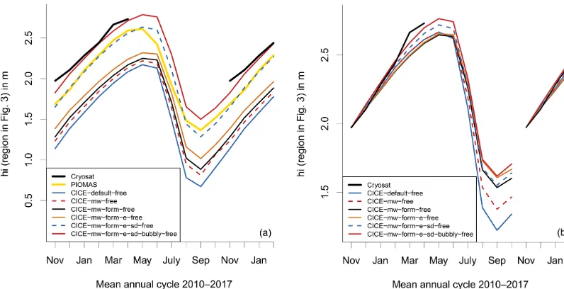
Comparing the CICE simulation with CS2 reveals that CICE-default underestimates the mean monthly sea ice thickness by about 0.8 m (see Fig. 1a and discussion in Sect. 4). This motivates experiments with perturbed physical parameteri-zations aiming to increase ice thickness. All additional sim-ulations are listed and described in Table 1. They have been performed as multi-year simulations (1980 to 2017, CICE-free) and seven 1-year-long simulations initialized with CS2 ice thickness (CICE-ini).
3.3.2 Uncertainty in atmospheric forcing data
We perform two sensitivity experiments to explore the im-pact of uncertainty in atmospheric forcing on simulated sea ice conditions: a decrease of incoming longwave radiation by 15 % and a decrease of 2 m air temperature by 2 K during the whole simulation. For both experiments, seven 1-year-long simulations are performed which are initialized with CS2 ice thickness (CICE-ini) in mid-November. The set-up of the ref-erence run has been applied (CICE-default). See Table 2 for details.
3.3.3 Impact of initial conditions and atmospheric forcing data
Table 1.Simulations with perturbed physical parameterizations improving sea ice thickness. Note that all model changes are cumulative. “Free” indicates multi-year simulations from 1980 to 2017; “ini” indicates the seven 1-year-long simulations starting in mid-November with CS2 sea ice thickness (2010/11 to 2016/17).
Run name Description free ini
CICE-mw The maximum meltwater added to melt ponds, rfracmax, is reduced from 100 % to 50 %. The
actual fraction of meltwater, rfrac, is calculated as rfrac=rfracmin+(rfracmax−rfracmin)× aice, with rfracmin=15 % and ice concentration aice. This reduction accounts for the uncer-tainty in the fraction of meltwater that collects in ponds versus being immediately released to the ocean. The impact of this change on the simulated melt pond fraction in July 2012 is demon-strated in Fig. 1. The melt pond fraction in the central Arctic is generally reduced by 5 %–10 %, ranging from 25 % to 40 % in the default simulation and from 20 % to 35 % in CICE-mw. The new melt pond distribution is more realistic with respect to MODIS-derived melt pond fractions (Roesel et al., 2012).
Y Y
CICE-mw-form Instead of a constant drag coefficient for the momentum fluxes between the atmosphere and
ice (CDa=1.3×10⁻³) and between ice and the ocean (CDo=5.36×10⁻³), the form drag parametrization of Tsamados et al. (2014) is applied, accounting for the impact of pressure ridges, keels, ice floe, and melt pond edges. Here, we modify the background drag coefficient for the atmosphere (csa=0.01 instead of 0.005) and the ocean (csw=0.0005 instead of 0.02)
and the parameters determining the impact of ridges and keels (cra=0.1 instead of 0.2 and
crw=0.5 instead of 0.2). These modifications increase ice drift over level ice and decrease ice drift over ridged ice, resulting in a more realistic ice drift pattern in comparison to Pathfinder (not shown).
Y Y
CICE-mw-form-e The longwave emissivity of sea ice is increased from 0.95 to 0.976. Y Y
CICE-mw-form-e-sd Depending on wind speed, snow density, and surface topography, snow can be eroded from
the sea ice surface, drift through air, and be redistributed or lost in leads. The default CICE simulation does not account for these processes. Here, we parameterize the snow erosion rate following Lecomte et al. (2014):
∂hs ∂t = −
γ
σITD V−V
∗ρs, MAX−ρs ρs2 ,
with snow depthhs, mass flux tuning coefficientγ=10−5kg m−2, current wind speedV,
threshold wind speedV∗=3.5 m s−1, current snow densityρs and maximum snow density
ρs,MAX, and standard deviation of ice thickness distributionσITD. Lacking information about
the snow density distribution, we apply ρs,MAX=330 kg m3 (the constant snow density in
CICE) and assumeρs=240 kg m3. Regarding the ITD, we applyσ values of 0.25 m for ice
category 1 (ice thicknessh <0.6 m), 0.5 m for category 2 (0.6 m< h <1.4 m), and 1 m for cat-egory 3 (1.4 m< h <2.4 m). We assume that the whole amount of snow blown into the air will be released into the ocean. Estimating the error of this assumption, we calculate the net snow re-deposition rate. Snow which is blown into air will be deposited at the surface and might be blown into the air again if the wind speed stays above the threshold value. Assuming an aver-age friction velocity of 0.1 m s−1and a total distance of 200 m, one cycle takes approximately 30 min. For every cycle, the lead fraction defines the fraction of snow volume released into the ocean. Analysing NCEP-2 wind fields, the average period the wind speed stays above the threshold value of 3.5 m s−2ranges from 50 to 120 h over the Arctic sea ice, with the lowest values close to the coast of North Greenland. Thus, for most parts of the Arctic more than 90 % of the total snow blown into the air would be lost in leads. An error of less than 10 % justi-fies our simplification. The impact of our parameterization on the simulated snow depth can be seen in Fig. 2. Accounting for the loss of drifting snow reduces the snow depth between 20 % and 40 %. The larger differences occur over regions with strongest winds and the smallest differences north of Greenland and Canada.
Y Y
CICE-mw-form-e-sd-bubbly (CICE-best)
We apply the bubbly conductivity formulation from Pringle et al. (2007), which results in larger thermal conductivity values for colder ice temperatures.
Figure 1.Impact of CICE set-up on mean effective sea ice thickness over the region shown in Fig. 3 and averaged over winter periods
2010/11 to 2016/17:(a)CICE-free simulations (multi-year runs from 1980 to 2017) and(b)CICE-ini simulations (seven 1-year-long runs
starting in mid-November with CS2 sea ice thickness). Model results are compared with mean sea ice thickness from CS2 CPOM and PIOMAS. Effective ice thickness (divided by ice concentration) is presented. For CS2 ice concentration is applied from CICE-default (mean values for November to April vary between 99.4 % and 99.8 %). See Sect. 3.3.1 for explanation of CICE % experiments. Note that results for November, December, January, and February are shown twice for improved visualization of the annual cycle.
Table 2.Sensitivity simulations exploring the impact of uncertainty in atmospheric forcing data. “Free” indicates multi-year simulations from 1980 to 2017; “ini” indicates seven 1-year-long simulations starting in mid-November with CS2 sea ice thickness (2010/11 to 2016/17).
Run name Description free ini
CICE-Ldown15 As CICE-default, but forcing
field incoming longwave radiation has been decreased by 15 % everywhere and for all times.
N Y
CICE-Tair2 As CICE-default, but forcing
field 2 m air temperature has been decreased by 2 K everywhere and for all times.
N Y
4 Results
4.1 Defining region for comparing model sea ice thickness with CryoSat-2 data
Several factors lead to errors in ice thickness retrieval from CS2, in particular the assumption of a climatological snow depth. The resulting ice thickness error is about 5 times larger than the error in snow depth; e.g. an underestimation in snow depth of 0.1 m leads to an underestimation in ice thickness of 0.5 m for a typical ice freeboard of 0.2 m (Tilling et al., 2015).
To enable a meaningful comparison of simulated sea ice thickness between CICE and CS2, we have to reduce the impact of errors. While for individual years and regions the W99 snow load can differ from reality by more than 0.1 m (Warren et al., 1999), the average snow conditions are accu-rately represented, at least over multi-year ice (e.g. Haas et al., 2017). Over first-year ice, snow depth is overestimated (Kurtz and Farrell, 2011; Webster et al., 2014); hence CS2 retrievals halve W99 snow depth (Sect. 1). We will compare multi-year monthly means over the CS2 period 2010 to 2017. Further, we compare spatial averages of ice thickness to re-duce the impact of random errors. A recent study by Nandan et al. (2017) showed that a vertical shift in the scattering hori-zon due to snow salinity could lead to an overestimation of CS2 ice thickness over first-year ice. Our region combines multi-year ice and first-year sea ice with a ratio of 65:35.
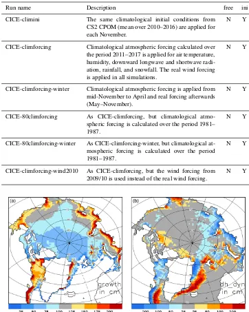
Table 3.Sensitivity simulations exploring the impact of initial and forcing conditions. “Free” indicates multi-year simulations from 1980 to 2017; “ini” indicates seven 1-year-long simulations starting in mid-November with CS2 sea ice thickness (2010/11 to 2016/17). The model configuration for all simulations is CICE-best.
Run name Description free ini
CICE-climini The same climatological initial conditions from
CS2 CPOM (mean over 2010–2016) are applied for each November.
N Y
CICE-climforcing Climatological atmospheric forcing calculated over
the period 2011–2017 is applied for air temperature, humidity, downward longwave and shortwave radi-ation, rainfall, and snowfall. The real wind forcing is applied in all simulations.
N Y
CICE-climforcing-winter Climatological atmospheric forcing is applied from
mid-November to April and real forcing afterwards (May–November).
N Y
CICE-80climforcing As CICE-climforcing, but climatological
atmo-spheric forcing is calculated over the period 1981– 1987.
N Y
CICE-80climforcing-winter As CICE-climforcing-winter, but climatological
at-mospheric forcing is calculated over the period 1981–1987.
N Y
CICE-climforcing-wind2010 As CICE-climforcing, but the wind forcing from
2009/10 is used instead of the real wind forcing.
N Y
Figure 2.Mean simulated sea ice thickness change from November to April (2010–2016) in CICE-default:(a)sea ice growth in centimetres and(b)sea ice thickness change by dynamical processes dh_dyn in centimetres (advection, convergence, and ridging).
impact is below±0.25 m in the central Arctic, more than 2 m of ice is exported on average from some coastal regions and transported to the Fram Strait (see Fig. 2b). For our region of interest, we only select grid cells in which the impact of dynamics on sea ice thickness change during winter is less than 0.25 m in magnitude. The resulting comparison region restricted by CS2 observations and dynamical sea ice change is shown in Fig. 3. We use this region for the rest of the paper.
4.2 Comparison of default CICE simulation with CryoSat-2 data
Figure 3. Region for comparing CICE and CS2 sea ice thickness where impact of winter growth on thickness change dominates other factors and where CS2 data are most accurate (see Sect. 4.1 for more details).
inter-annual variability of, e.g. the September ice extent. The magnitude of the ice thickness difference of 0.8 m cannot be explained by the uncertainty of the CS2 ice thickness alone (Tilling et al., 2016; Stroeve et al., 2018) and so indicates a model error.
CS2 ITD can be applied to initialize a CICE simulation with the observed ice thickness and CS2 data enable us to trace the ice thickness continuously through the whole win-ter until April. We apply the mean November CS2 ITD to ini-tialize the CICE simulations in mid-November for the years from 2010 to 2016. Starting in mid-November, the mean sim-ulated April ice thickness from CICE-ini-default is about 0.25 m too thin (Fig. 1b). This indicates that the winter ice growth is underestimated in the model. To explore the rea-sons for the underestimation, we will first examine the impact of atmospheric forcing data (Sect. 4.3) and then the impact of the physical processes involved and how they are represented in CICE (Sect. 4.4).
4.3 Impact of uncertainty in atmospheric forcing data CICE ice growth in the central Arctic mainly depends on at-mospheric forcing (in particular incoming longwave radia-tion and air temperature), the parameterizaradia-tion of the turbu-lent atmospheric heat fluxes (heat transfer coefficients), and the conductive heat fluxes within the ice and snow layers. While the impact of the turbulent ocean heat flux under the ice can be large in the marginal ice zone, the ocean tempera-ture is generally close to the freezing temperatempera-ture in the cen-tral Arctic during winter.
To explore to what extent the underestimation of ice thick-ness can be attributed to errors in the surface energy bal-ance associated with atmospheric forcing data, we performed two sensitivity studies in which we decreased (1) the incom-ing longwave radiation by 15 W m−2 (CICE-Ldown15-ini) and (2) the 2 m air temperature (CICE-Tair2-ini) during the
whole simulation period and for every location (see Table 2). We have chosen these values as estimates for potential total systematic atmospheric errors (e.g. Chaudhuri et al., 2014). The impact of these atmospheric perturbations on ice growth is small (see Fig. 5) and the gap between CS2 ice thick-ness and CICE-default ice thickthick-ness can only be reduced marginally. The reduced longwave radiation and air tempera-ture lead to a reduction of ice surface temperatempera-ture in the range of 2 to 3 K and only increase ice growth by about 5 % each. This is due to the fact that surface temperatures are around −30◦C during winter and the conductivity of the snow layer is low. Winter ice growth is not strongly affected by errors in atmospheric conditions. This is fundamentally different dur-ing the meltdur-ing season. Figure 5 reveals that the sea ice would be 0.9 m thicker in September due to the reduction of incom-ing longwave radiation and 1.4 m thicker due to the decrease of 2 m air temperature, starting with the same initial condi-tions in the November of the previous year. These sensitivity studies reveal that the underestimation of winter ice growth cannot be explained by errors in the surface energy balance associated with atmospheric forcing data.
4.4 Improving CICE simulation by varying model physics
In the sea ice model, local ice thickness changes are calcu-lated by thermodynamic processes (ice growth and melt) and dynamic processes (advection and ridging). The thermody-namic change depends on the energy balance at the interfaces between the atmosphere, snow, ice, and the ocean derived from the shortwave and longwave radiation fluxes, the turbu-lent heat fluxes, and the conductive heat flux through the ice and snow. Addressing the individual contributions systemat-ically, we alter model physics within their range of uncer-tainty with the aim to increase sea ice thickness. Our model changes are presented in a cumulative way.
melt-Figure 4.Difference in mean September sea ice concentration (2005–2014) in % between the CICE simulation and SSM/I Bootstrap data. Negative values mean lower ice concentration in CICE. The black line indicates mean SSM/I and the red line the mean CICE sea ice extent:
(a)CICE-default and(b)CICE-best.
Figure 5.Impact of uncertainty in atmospheric forcing on simulated mean effective sea ice thickness over the region shown in Fig. 3 and averaged over winter periods 2010/11 to 2016/17. CICE-ini simula-tions: default, default with increase of incoming longwave radiation of 15 W m−2, default with increase of 2 m air temperature of 2 K (everywhere and anytime), and best. Model results are compared with mean sea ice thickness from CS2 CPOM.
water. Figure 1a shows that the thickness error is marginally reduced by CICE-mw from about 0.8 to 0.70–0.75 m. As ex-pected there is no impact during winter for the initialized simulation, but the summer ice is 0.2 m thicker (Fig. 1b).
In the next experiment, we address the sea ice advection and the turbulent heat fluxes. We apply the form drag pa-rameterization of Tsamados et al. (2014) in addition to the release of more meltwater (CICE-mw-form). Ice thickness increased slightly with respect to CICE-mw due to a reduced ice drift speed, resulting in a weaker ocean–ice heat flux and less ice export. In addition, increasing the emissivity of
snow and ice from 0.95 to 0.976 (CICE-mw-form-e) affects the longwave radiation budget. The increase reduces summer melt by a few centimetres, but no impact during winter is vis-ible.
Due to its low conductivity, snow depth controls the con-ductive heat flux. Here, we implement a snow drift scheme based on Lecomte et al. (2014) which reduces the snow depth by 20 % to 40 % (CICE-mw-form-e-sd; see Fig. 7) and has the biggest impact on sea ice thickness from all individual changes. With respect to CICE-default, the thickness error has been reduced from 0.8 to 0.25 m (see CICE-mw-form-e-sd-free in Fig. 1a). The reduction of snow depth leads to a strong increase in ice growth in winter, but also to a moderate increase of summer melt due to an earlier disappearance of snow. This can be seen comparing CICE-mw-form-e-sd-ini with CICE-mw-form-e-ini in Fig. 1b. The reduction of snow leads to an increase of May ice thickness of 0.12 m and to a decrease of September ice thickness of 0.06 m. Applying an increased conductivity coefficient for colder temperature (Pringle et al., 2007; CICE-mw-form-e-sd-bubbly) in addi-tion reduces the error for CICE-free and CICE-ini to less than 0.1 m. This modification increases winter ice growth, but it has no impact during summer.
Figure 6.Impact of reduced retained meltwater fraction on simulated melt pond area fraction in July 2012:(a)CICE-default and(b) CICE-mw.
Figure 7.Impact of snow erosion on simulated mean April snow depth (2010 to 2017):(a)CICE-default and(b)CICE-mw-from-e-sd.
Table 4.Mean area fraction of sea ice per category in % according to CS2 and CICE-best-ini (over the region shown in Fig. 3 and for the period 2010 to 2017).
Ice thickness (h) CS2 CS2 CICE-best-ini
category November April April
1 (h <0.6 m) 8 5 2
2 (0.6 m< h <1.4 m) 17 7 4
3 (1.4 m< h <2.4 m) 43 23 30
4 (2.4 m< h <3.6 m) 27 42 54
5 (h >3.6 m) 4 22 10
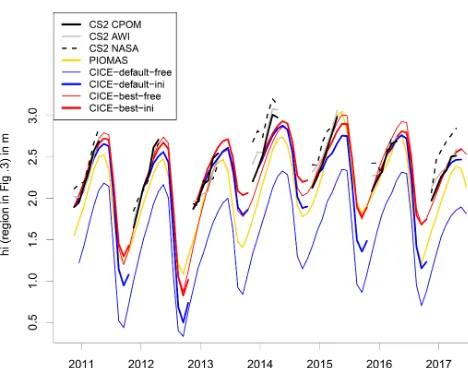
So far, we have compared the mean annual cycle of sea ice thickness over the period from 2010 to 2017. Figure 8 com-pares times series of the individual years from free and ini-tialized CICE simulations with three different CS2 products provided by CPOM, AWI and NASA. For all years, CICE-best-free is much closer to CS2 than CICE-default-free. It is
striking that differences between best-free and CICE-best-ini are small. This is a remarkable result from a mod-elling point of view because it means that CICE-best is so realistic that the assimilation of sea ice thickness would not result in substantial changes. This agreement increases the confidence in our new model set-up.
differ-Figure 8.Mean effective sea ice thickness over the region shown in Fig. 3. Verification of CICE-free default and best (thin lines) and CICE-ini default and best (thick lines) with CS2 CPOM, AWI, NASA, and PIOMAS.
ences between PIOMAS, CS2, and CICE-best in the sea ice thickness evolution, the general statement that CICE-best is more realistic than CICE-default is confirmed by PIOMAS.
As the summer sea ice extent is quite realistic in CICE-default (Sect. 4.2), we investigate the impact of the strong ice thickness increase in CICE-best on sea ice concentration and extent. Figure 4a reveals that the mean September sea ice extent over the period 2005–2014 is slightly underestimated in CICE-default with respect to SSM/I Bootstrap (Comiso, 1999). The impact of the strong thickness increase on sea ice extent is small; the ice extent is only marginally larger in CICE-best (Fig. 4b), but nevertheless close to SSM/I Boot-strap. In contrast to ice extent, ice concentration is underesti-mated in CICE-default by 25 % to 50 % in large parts of the ice-covered Arctic Ocean. While apart from the ice edge, ice concentration is generally between 80 % and 100 % accord-ing to SSM/I Bootstrap, CICE-default frequently shows large areas with values below 50 %. This discrepancy is strongly reduced in CICE-best, with error values below 10 % in the Canadian half and between 10 % and 30 % in the Siberian half of the Arctic (Fig. 4b). It is worth mentioning that nearly all CMIP5 climate models underestimate Arctic sum-mer sea ice concentration in their historical runs with respect to SSM/I Bootstrap (see e.g. Fig. 3 in Notz, 2014). CICE-best does not only improve the sea ice thickness, but also the summer sea ice concentration.
We demonstrate the impact of our model changes on the timing of mean melt and freeze onset (2005–2014) between CICE-best and CICE-default in Fig. 9. In CICE-best, the melt onset day is later (0–4 days in the central Arctic, up to 10 days in the Fram Strait) and the freeze onset is ear-lier (4–12 days in most areas), resulting in a shorter melt-ing season. The simulated mean length of the meltmelt-ing
sea-Table 5.Impact of initial November sea ice conditions and atmo-spheric forcing on the mean sea ice thickness (hi) of subsequent April and September over the region shown in Fig. 3 from 2011 to 2017. See Sect. 3.3 for explanation of CICE simulations. Inter-annual variability is given in parentheses.
Set-up April hi in m September hi in m
CICE-ini 2.70 (±0.18) 1.62 (±0.50) CICE-clim-ini 2.67 (±0.10) 1.57 (±0.40) CICE-climforcing-ini 2.70 (±0.17) 1.90 (±0.25) CICE-climforcing-winter-ini 2.70 (±0.17) 1.62 (±0.50) CICE-80climforcing-ini 2.81 (±0.16) 2.37 (±0.21) CICE-80climforcing-winter-ini 2.81 (±0.16) 1.78 (±0.49) CICE-climforcing-wind2010-ini 2.57 (±0.17) 1.92 (±0.17)
son over the Arctic Basin reduces from 107 days (CICE-default) to 100 days (CICE-best). This is an improvement with respect to the observed value of 94 days. The observed number of 94 days is based on a mean value of 88 days for the period 1979 to 2012 and accounting for the trend of 3.7 days decades−1(Stroeve et al., 2014). The impact of the model changes is remarkable given that we apply the same 2 m air temperature data (NCEP-2) as atmospheric forcing. Our examples indicate that the chosen model physics may be important for many climate-related questions and how cli-mate models predict future changes of summer melting sea-son and sea ice decline.
4.5 Impact of initial conditions and atmospheric forcing
How strongly do the CICE simulations depend on sea ice initial conditions? Using the mean CS2 November sea ice thickness from 2010 to 2016 (CICE-climini; Table 3) instead of the annual values leads to positive or negative thickness anomalies which remain throughout the year, becoming only slightly weaker during winter (Fig. 10). The inter-annual variability of the simulated April ice thickness is reduced by 44 % (from 0.18 to 0.10 m, Table 5) and the September ice thickness by 20 % (from 0.5 to 0.4 m).
Applying a mean atmospheric forcing for each year (CICE-climforcing-ini) hardly affects the ice thickness dur-ing winter (with the exception of winter 2016/17), but it leads to strong anomalies during summer (Fig. 10). The mean September sea ice thickness is increased by 0.28 m and the inter-annual variability reduced from 0.5 to 0.25 m (Table 5). Applying the mean atmospheric forcing during winter only and the individual atmospheric forcing from May onwards (CICE-climforcing-winter-ini), sea ice thickness during sum-mer is nearly unchanged with respect to CICE-ini. While the atmospheric conditions during summer are decisive for summer ice melt and September sea ice thickness, the atmo-spheric winter conditions seem not to matter at all.
Figure 9.Difference in mean melt onset(a)and freeze onset(b)on days between CICE-best and CICE-default (2010–2017). Positive values mean a later onset day in CICE-best.
Figure 10.Impact of climatological initial conditions (climini), cli-matological forcing (climforcing), and clicli-matological forcing dur-ing winter only (November to April, climforcdur-ing-winter). All CICE simulations from CICE-ini best. Mean effective sea ice thickness over the region is shown in Fig. 3. CS2 as in Fig. 7. The climatology is calculated over the period 2011 to 2017 for air temperature, hu-midity, downward longwave and shortwave radiation, rainfall, and snowfall. The real wind forcing is applied in all simulations.
Is it possible that the small variability of these winter periods could cause the weak impact on sea ice thickness? To exclude this possibility, we perform additional sensitivity experi-ments in which we apply colder atmospheric conditions from the 1980s (CICE-80climforcing-ini). Figure 11 and Table 3 reveal that the impact during winter is nevertheless small (mean thickness increase of 0.11 m), but huge in summer (+0.8 m). Interestingly, the impact of using the wind forc-ing from an anomalous year (2009/10, stronger transpolar-drift), CICE-climforcing-wind20100ini, is stronger on April ice thickness (−0.13 m) than from the cold atmospheric
con-Figure 11.As Fig. 10, but applying a climatology calculated over the period 1981 to 1987.
ditions. This confirms the important role of sea ice dynamics and export through the Fram Strait in controlling the sea ice volume variability (Ricker et al., 2018).
These sensitivity experiments demonstrate that the atmo-spheric winter conditions have a very small impact on winter ice growth and thus on April ice thickness. September ice thickness depends strongly on atmospheric conditions from May to September.
5 Conclusions
proportion-ally less accurate, we exclude locations where sea ice dynam-ics (sea ice advection and ridging) make a strong contribution to the modification of sea ice thickness. We further exclude locations where the number of CS2 observations is limited and the sea ice is thin during winter (<0.5 m). The resulting region includes most of the central Arctic, but not the area of the thickest ice north of Canada or any of the shelf seas (see Fig. 3).
Comparing the multi-year means reveals that CICE-default underestimates ice thickness over our comparison re-gion by about 0.8 m (see Fig. 1a). This discrepancy would not have been identified by comparing total Arctic ice vol-ume. Due to overestimating ice thickness in the Canadian sector, Arctic ice volume from CICE-default is only slightly lower than estimates based on CS2 or PIOMAS. Deriving the sub-grid-scale ice thickness distribution (ITD) from CS2 al-lows us to initialize CICE simulations with the identical ice thickness in November. Applying default settings CICE-ini underestimates mean ice thickness in the following April by 0.25 m (see Fig. 1b). This indicates that the winter ice growth is too weak in the model. What is the reason for the underes-timation of ice growth? Our sensitivity experiments give ev-idence that uncertainty in atmospheric forcing cannot be the main reason. The impact of errors in air temperature and in-coming longwave radiation on sea ice growth is rather small in winter (see Fig. 5). The turbulent ocean–ice heat flux is generally small in winter in the central Arctic; thus, errors deriving from the turbulent ocean–ice heat flux cannot be re-sponsible either. The ice–atmosphere heat fluxes depend on atmospheric forcing and the transfer coefficients. Varying the transfer coefficients does not result in major changes of sea ice growth. Initial conditions in autumn are important, but our initialized CICE simulations show that April ice thick-ness is still underestimated even when starting with the “cor-rect” November ice thickness. Thus, by a process of exclu-sion, we conclude that sea ice physics related to the conduc-tive flux must be responsible.
The strongest contribution to the simulation of winter ice growth comes from implementing a snow drift scheme based on Lecomte et al. (2014). Although our implementation is simple and further work to improve the parameterization is required, it demonstrates the importance of including addi-tional snow processes in sea ice models for climate appli-cations (Vionnet et al., 2012; Nandan et al., 2017; Liston et al., 2018). Such model development can also benefit recent Arctic-wide snow products that rely on satellite observations (Maaß et al., 2013; Guerreiro et al., 2016; Lawrence et al., 2018) or reanalysis precipitation fields that rely on drifting sea ice (Kwok and Cunningham, 2008).
Our sensitivity experiments modifying initial and atmo-spheric forcing data reveal that ice thickness anomalies in November decay over winter but are still present in the fol-lowing April (see Fig. 10). Comparing inter-annual vari-ability of April ice thickness between ini and CICE-climini (Table 5) shows that half of the variability comes
from the initial conditions. Atmospheric conditions during spring and summer are decisive for summer sea ice condi-tions, but atmospheric winter conditions have little impact on sea ice growth. Using “cold” forcing from the 1980s instead of the more recent winters leads to an increase in September sea ice thickness of 0.8 m, but only to an increase in April ice thickness of 0.11 m (see Fig. 11 and Table 5). This reflects the importance of feedback processes. During winter, the negative conductive feedback process (less ice, more growth) is dominating, while during summer the pos-itive albedo feedback process determines sea ice changes. The impact of the negative winter feedback has been dis-cussed in Stroeve et al. (2018). In their study, a potential weakening of the feedback during the last years has been raised as a question. Here, we answer this question, demon-strating that warm winters are not important for observed sea ice thinning in recent decades, at least in the central Arctic. The situation can be different in the marginal win-ter sea ice zone, where a warm winwin-ter can increase mixed-layer ocean temperature and delay ice growth. Our find-ings are in agreement with observations of recent years: in spite of the three warmest Arctic-wide winter air tem-peratures during 2014/15, 2015/16, and 2016/17 on record (Stroeve et al., 2018), the September Arctic sea ice extent in 2015 (4.7 million km2), 2016 (4.7 million km2), and 2017 (4.9 million km2) was larger than in 2012 (3.6 million km2); these numbers are based on SSM/I NASA-Team algorithm (Cavalieri et al., 1996, updated 2017). We conclude that the fate of Arctic summer sea ice depends largely on atmospheric spring and summer conditions, in particular May and June, when the melting season starts and melt ponds form, precon-ditioning the strength of the positive albedo feedback mech-anism (Schröder et al., 2014).
Our optimal model configuration CICE-best does not only improve the simulation of mean sea ice thickness over the central Arctic with respect to CS2, but also improves summer sea ice concentration (in comparison to SSM/I Bootstrap), the length of the melt season (in comparison to Stroeve et al., 2014), and the melt pond fraction (in comparison to MODIS and MERIS). Recent studies have demonstrated improve-ments for sea ice predictions up to 6 months, initializing fore-cast models with CS-2 data (Allard et al., 2018; Blockley and Peterson, 2018). Here, we show that our improvements to the sea ice model CICE are so fundamental and consistent that any differences between CICE simulations initialized by CS2 ice thickness and those which do not utilize them are mini-mized. It is the first time CS2 sea ice thickness data have been applied successfully to improve sea ice model physics.
seaice.html (last access: December 2017), NASA data are avail-able from: https://nsidc.org/data/RDEFT4/ (Kurtz and Harbeck, 2017). NCEP2 data obtained from NOAA Earth System Research Laboratory (http://www.esrl.noaa.gov/psd/data/gridded/data.ncep. reanalysis2.gaussian.html, last access: December 2017).
Author contributions. AR, RT, and MT prepared the Cyrosat-2 data. DS performed the CICE simulations. All authors contributed to the composition of the paper and the discussion of the results.
Competing interests. The authors declare that they have no conflict of interest.
Acknowledgements. This work was done under the ACSIS and UKESM program funded by the UK Natural Environment Research Council. The authors would like to thank the Isaac Newton Institute for Mathematical Sciences for support and hospitality during the programme Mathematics of Sea Ice Phenomena, when work on this paper was undertaken. This work was supported by EPSRC grant number EP/K032208/1. Michel Tsamados acknowledges the
support from the Arctic+European Space Agency snow project
ESA/AO/1-8377/15/I-NB NB – STSE – Arctic+.
Edited by: John Yackel
Reviewed by: two anonymous referees
References
Allard, R. A., Farrell, S. L., Hebert, D. A., Johnston, W. F., Li, L., Kurtz, N. T., Phelps, M. W., Posey, P. G., Tilling, R., Ridout, A., and Wallcraft, A. J.: Utilizing CryoSat-2 sea ice thickness to initialize a coupled ice-ocean modeling system, Adv. Space Res., 62, 1265–1280, https://doi.org/10.1016/j.asr.2017.12.030, 2018. Bauer, M., Schröder, D., Heinemann, G., Willmes, S., and Ebner, L.: Quantifying polynya ice production in the Laptev Sea with the COSMO model, Polar Res., 32, 20922, https://doi.org/10.3402/polar.v32i0.20922, 2013.
Bitz, C. and Lipscomb, W.: An energy-conserving thermody-namic model of sea ice, J. Geophys. Res., 104, 15669–15677, https://doi.org/10.1029/1999JC900100, 1999.
Blockley, E. W. and Peterson, K. A.: Improving Met Of-fice seasonal predictions of Arctic sea ice using assimila-tion of CryoSat-2 thickness, The Cryosphere, 12, 3419–3438, https://doi.org/10.5194/tc-12-3419-2018, 2018.
Briegleb, B. P. and Light, B.: A delta-Eddington multiple scattering parameterization for solar radiation in the sea ice component of the Com- munity Climate System Model, Tech. Note 472, Natl. Cent. for Atmos. Res., Boulder, CO, 2007.
Cavalieri, D., Parkinson, C., Gloersen, P., and Zwally, H. J.: Sea Ice Concentrations from Nimbus-7 SMMR and DMSP SSM/I-SSMIS Passive Microwave Data, Boulder, Colorado USA, NASA DAAC at the National Snow and Ice Data Center, 1996 (updated 2017).
Chaudhuri, A. H., Ponte, R. M., and Nguyen, A. T.: A Comparison of Atmospheric Reanalysis Products for the Arctic Ocean and
Implications for Uncertainties in Air-Sea Fluxes, J. Climate, 27, 5411–5421, https://doi.org/10.1175/JCLI-D-13-00424.1, 2014. Comiso, J.: Bootstrap Sea Ice Concentrations From NIMBUS-7
SMMR and DMSP SSM/I, available at: http://nsidc.org/data/ nsidc-0079.html (last access: December 2017), Natl. Snow and Ice Data Cent., Boulder, CO, 1999 (updated 2017).
Dmitrenko, I. A., Kirillov, S. A., Tremblay L. B., Bauch, D., and Willmes, S.: Sea-ice production over the Laptev Sea Shelf inferred from historical summer-to-winter hydrographic obser-vations of 1960s to 1990s, Geophys. Res. Lett. 36, L13605, https://doi.org/10.1029/2009GL038775, 2009.
Ferry, N., Masina, S., Storto, A., Haines, K., Valdivieso, M., Barnier, B., and Molines, J.-M.: Product User Manual GLOBAL-REANALYSISPHYS-001-004-a and b, MyOcean, 2011. Flocco, D., Feltham, D. L., and Turner, A. K.: Incorporation of
a physically based melt pond scheme into the sea ice com-ponent of a climate model, J. Geophys. Res., 115, C08012, https://doi.org/10.1029/2009JC005568, 2010.
Flocco, D., Schröder, D., Feltham, D. L., and Hunke, E. C.: Impact of melt ponds on Arctic sea ice simula-tions from 1990 to 2007, J. Geophys. Res., 117, C09032, https://doi.org/10.1029/2012JC008195, 2012.
Giles, K. A., Laxon, S. W., Wingham, D. J., Wallis, D. W., Kra-bill, W. B., Leuschen, C. J., McAdoo, D., Manizade, S. S., and Raney, R. K.: Combined airborne laser and radar altimeter mea-surements over the Fram Strait in May 2002, Remote Sens. En-viron., 111, 182–194, https://doi.org/10.1016/j.rse.2007.02.037, 2007.
Giles, K. A., Laxon, S. W., and Ridout, A. L.: Circumpo-lar thinning of Arctic sea ice following the 2007 record ice extent minimum, Geophys. Res. Lett., 35, L22502, https://doi.org/10.1029/2008GL035710, 2008.
Guerreiro, K., Fleury, S., Zakharova, E., Rémy, F., and Kouraev, A.: Potential for estimation of snow depth on Arctic sea ice from CryoSat-2 and SARAL/AltiKa missions, Remote Sens. Environ., 186, 339–349, 2016.
Haas, C., Beckers, J., King, J., Silis, A., Stroeve, J., Wilkinson, J., Notenboom, B., Schweiger, A., and Hendricks, S.: Ice and snow thickness variability and change in the high Arctic Ocean ob-served by in situ measurements, Geophys. Res. Lett., 44, 10462– 10469, https://doi.org/10.1002/2017GL075434, 2017.
Hendricks, S., Ricker, R., and Helm, V.: User Guide – AWI CryoSat-2 Sea Ice Thickness Data Product (v1.2), hdl:10013/epic.48201, 2016.
Heorton, H., Feltham, D. L., and Tsamados, M.: Stress and deformation characteristics of sea ice in a high resolu-tion, anisotropic sea ice model, Phil. Trans A, 376, 2129, https://doi.org/10.1098/rsta.2017.0349, 2018.
Hunke, E. C., Lipscomb, W. H., Turner, A. K., Jeffery, N., and El-liott, S.: CICE: the Los Alamos Sea Ice Model Documentation and Software User’s Manual Version 5.1, 2015.
Kanamitsu, M., Ebisuzaki, W., Woollen, J., Yang, S.-K., Hnilo, J. J., Fiorino, M., and Potter, G. L.: NCEP-DOE AMIP-II Reanalysis (R-2), B. Am. Meteorol. Soc., 83, 1631–1643, 2017.
Kurtz, N. T. and Farrell, S. L.: Large-scale surveys of snow depth on Arctic sea ice from Operation IceBridge, Geophys. Res. Lett., 38, L20505, https://doi.org/10.1029/2011GL049216, 2011. Kurtz, N. T., Farrell, S. L., Studinger, M., Galin, N., Harbeck, J. P.,
Lindsay, R., Onana, V. D., Panzer, B., and Sonntag, J. G.: Sea ice thickness, freeboard, and snow depth products from Oper-ation IceBridge airborne data, The Cryosphere, 7, 1035–1056, https://doi.org/10.5194/tc-7-1035-2013, 2013.
Kurtz, N. T., Galin, N., and Studinger, M.: An improved CryoSat-2 sea ice freeboard retrieval algorithm through the use of waveform fitting, The Cryosphere, 8, 1217–1237, https://doi.org/10.5194/tc-8-1217-2014, 2014.
Kurtz, N. T. and Harbeck, J.: CryoSat-2 Level 4 Sea Ice Elevation, Freeboard, and Thickness, Version 1, Boulder, Colorado USA, NASA National Snow and Ice Data Center Distributed Active Archive Center, 2017.
Kwok, R. and Rothrock, D. A.: Decline in Arctic sea ice thickness from submarine and ICESat records: 1958–2008, Geophys. Res. Lett., 36, L15501, https://doi.org/10.1029/2009GL039035, 2009. Kwok, R. and Cunningham, G. F.: ICESat over Arctic sea ice: Estimation of snow depth and ice thickness, J. Geophys. Res.-Oceans, 113, https://doi.org/10.1029/2008JC004753, 2008. Lawrence, I. R., Tsamados, M. C., Stroeve, J. C., Armitage, T.
W. K., and Ridout, A. L.: Estimating snow depth over Arc-tic sea ice from calibrated dual-frequency radar freeboards, The Cryosphere, 12, 3551–3564, https://doi.org/10.5194/tc-12-3551-2018, 2018.
Laxon, S. W., Giles, K. A., Ridout, A. L., Wingham, D. J., Willatt, R., Cullen, R., Kwok, R., Schweiger, A., Zhang, J., Haas, C., Hendricks, S., Krishfield, R., Kurtz, N., Far-rell, S., and Davidson, M.: CryoSat-2 estimates of Arctic sea ice thickness and volume, Geophys. Res. Lett., 40, 732–737, https://doi.org/10.1002/grl.50193, 2013.
Lecomte, O., Fichefet, T., Flocco, D., Schröder, D., and Vancop-penolle, M.: Impacts of wind-blown snow redistribution on melt ponds in a coupled ocean – sea ice model, Ocean Model, 87, 67– 80, https://doi.org/10.1016/j.ocemod.2014.12.003, 2014. Lipscomb, W. H. and Hunke, E. C.: Modeling sea ice transport
using incremental remapping, Mon. Weather Rev., 132, 1341– 1354, 2004.
Liston, G. E., Polashenski, C., Roesel, A., Itkin, P., King, J., Merk-ouriadi, I., and Haapala, J.: A distributed snow-evolution model for sea-ice applications (SnowModel), J. Geophys. Res.-Ocean, 123, 3786–3810, https://doi.org/10.1002/2017JC013706, 2018. Maaß, N., Kaleschke, L., Tian-Kunze, X., and Drusch, M.: Snow
thickness retrieval over thick Arctic sea ice using SMOS satellite data, The Cryosphere, 7, 1971–1989, https://doi.org/10.5194/tc-7-1971-2013, 2013.
Massonnet, F., Fichefet, T., Goosse, H., Bitz, C. M., Philippon-Berthier, G., Holland, M. M., and Barriat, P.-Y.: Constraining projections of summer Arctic sea ice, The Cryosphere, 6, 1383– 1394, https://doi.org/10.5194/tc-6-1383-2012, 2012.
Maykut, G. A. and Untersteiner, N.: Some results from a time-dependent thermodynamic model of sea ice, J. Geophys. Res., 76, 1550–1575, https://doi.org/10.1029/JC076i006p01550, 1971.
Nandan, V., Geldsetzer, T., Yackel, J., Mahmud, M., Scharien, R., Howell, S., King, J., Ricker, R., and Else, B.: Effect of Snow Salinity on CryoSat-2 Arc- tic First-Year Sea Ice Free-board Measurements, Geophys. Res. Lett., 44, 10419–10426, https://doi.org/10.1002/2017GL074506, 2017.
Notz, D.: Sea-ice extent and its trend provide limited met-rics of model performance, The Cryosphere, 8, 229–243, https://doi.org/10.5194/tc-8-229-2014, 2014.
Pringle, D. J., Eicken, H., Trodahl, H. J., and Backstrom,
L. G. E.: Thermal conductivity of landfast
Antarc-tic and ArcAntarc-tic sea ice, J. Geophys. Res., 112, C04017, https://doi.org/10.1029/2006JC003641, 2007.
Rae, J. G. L., Hewitt, H. T., Keen, A. B., Ridley, J. K., Ed-wards, J. M., and Harris, C. M.: A sensitivity study of the sea ice simulation in HadGEM3, Ocean Model, 74, 60–76, https://doi.org/10.1016/j.ocemod.2013.12.003, 2014.
Ricker, R., Hendricks, S., Helm, V., Skourup, H., and Davidson, M.: Sensitivity of CryoSat-2 Arctic sea-ice freeboard and thick-ness on radar-waveform interpretation, The Cryosphere, 8, 1607– 1622, https://doi.org/10.5194/tc-8-1607-2014, 2014.
Ricker, R., Hendricks, S., Kaleschke, L., Tian-Kunze, X., King, J., and Haas, C.: A weekly Arctic sea-ice thickness data record from merged CryoSat-2 and SMOS satellite data, The Cryosphere, 11, 1607–1623, https://doi.org/10.5194/tc-11-1607-2017, 2017. Ricker, R., Girard-Ardhuin, F., Krumpen, T., and Lique, C.:
Satellite-derived sea ice export and its impact on Arc-tic ice mass balance, The Cryosphere, 12, 3017–3032, https://doi.org/10.5194/tc-12-3017-2018, 2018.
Ridley, J. K., Blockley, E. W., Keen, A. B., Rae, J. G. L., West, A. E., and Schroeder, D.: The sea ice model compo-nent of HadGEM3-GC3.1, Geosci. Model Dev., 11, 713–723, https://doi.org/10.5194/gmd-11-713-2018, 2018.
Rösel, A., Kaleschke, L., and Birnbaum, G.: Melt ponds on Arctic sea ice determined from MODIS satellite data us-ing an artificial neural network, The Cryosphere, 6, 431–446, https://doi.org/10.5194/tc-6-431-2012, 2012.
Rothrock, D. A.: The energetics of the plastic deformation of pack ice by ridging, J. Geophys. Res., 80, 4514–4519, https://doi.org/10.1029/JC080i033p04514, 1975.
Rothrock, D. A., Percival, D. B., and Wensnahan, M.: The decline in arctic sea-ice thickness: Separating the spa-tial, annual, and interannual variability in a quarter cen-tury of submarine data, J. Geophys. Res., 113, C05003, https://doi.org/10.1029/2007JC004252, 2008.
Schröder, D., Feltham, D. L., Flocco, D., and Tsamados,
M.: September Arctic sea-ice minimum predicted by
spring melt-pond fraction, Nat. Clim. Change, 4, 353–357, https://doi.org/10.1038/NCLIMATE2203, 2014.
Schröder, D.: Simulations with the sea ice model CICE document-ing the impact of improved sea ice physics, University of Read-ing, available at: http://dx.doi.org/10.17864/1947.187, 2018. Shu, Q., Song, Z., and Qiao, F.: Assessment of sea ice
simu-lations in the CMIP5 models, The Cryosphere, 9, 399–409, https://doi.org/10.5194/tc-9-399-2015, 2015.
Stroeve, J. C., Markus, T., Boisvert, L., Miller, J., and Bar-rett, A.: Changes in Arctic melt season and implications for sea ice loss, Geophys. Res. Lett., 41, 1216–1225, https://doi.org/10.1002/2013GL058951, 2014.
Stroeve, J. C., Schröder, D., Tsamados, M., and Feltham, D.: Warm winter, thin ice?, The Cryosphere, 12, 1791–1809, https://doi.org/10.5194/tc-12-1791-2018, 2018.
Tilling, R. L., Ridout, A., Shepherd, A., and Wingham, D. J.: In-creased arctic sea ice volume after anomalously low melting in 2013, Nat. Geosci., 8, 643–646, 2015.
Tilling, R. L., Ridout, A., and Shepherd, A.: Near-real-time Arctic sea ice thickness and volume from CryoSat-2, The Cryosphere, 10, 2003–2012, https://doi.org/10.5194/tc-10-2003-2016, 2016. Tilling, R. L., Ridout, A., and Shepherd, A.: Estimating
Arctic sea ice thickness and volume using CryoSat-2
radar altimeter data, Adv. Space Res., 62, 1203–1225, https://doi.org/10.1016/j.asr.2017.10.051, 2018.
Tsamados, M., Feltham, D. L., and Wilchinsky, A. V.:
Impact of a new anisotropic rheology on simulations
of Arctic sea ice, J. Geophys. Res., 118, 91–107,
https://doi.org/10.1029/2012JC007990, 2013.
Tsamados, M., Feltham, D. L., Schröder, D., Flocco, D., Farrell, S., Kurtz, N., Laxon, S., and Bacon, S.: Impact of variable atmo-spheric and oceanic form drag on simulations of Arctic sea ice, J. Phys. Oceanogr., 44 1329–1353, https://doi.org/10.1175/JPO-D-13-0215.1, 2014.
Vionnet, V., Brun, E., Morin, S., Boone, A., Faroux, S., Le Moigne, P., Martin, E., and Willemet, J.-M.: The detailed snow-pack scheme Crocus and its implementation in SURFEX v7.2, Geosci. Model Dev., 5, 773–791, https://doi.org/10.5194/gmd-5-773-2012, 2012.
Wang, X., Key, J., Kwok, R., and Zhang, J.: Comparison of Arctic Sea Ice Thickness from Satellites, Aircraft, and PIOMAS Data, Remote Sens., 8, 713, https://doi.org/10.3390/rs8090713, 2016. Warren, S. G., Rigor, I. G., Untersteiner, N., Radionov, V. F.,
Bryaz-gin, N. N., Aleksandrov, Y. I., and Barry, R.: Snow depth on Arc-tic sea ice, J. Climate, 12, 1814–1829, 1999.
Webster, M. A., Rigor, I. G., Nghiem, S. V., Kurtz, N. T., Farrell, S. L., Perovich, D. K., and Sturm, M.: Interdecadal changes in snow depth on Arctic sea ice, J. Geophys. Res.-Ocean, 119, 5395– 5406, https://doi.org/10.1002/2014JC009985, 2014.
Wilchinsky, A. V. and Feltham, D. L.: Modelling the rheology of sea ice as a collection of diamond-shaped floesAnisotropic model for granulated sea ice dynamics, J. Non-Newton. Fluid, 138, 22–32, https://doi.org/10.1016/j.jnnfm.2006.05.001, 2006.
Willatt, R., Laxon, S., Giles, K., Cullen, R., Haas, C., and Helm, V.: Ku-band radar penetration into snow cover Arctic sea ice us-ing airborne data, Ann. Glaciol., 57, 197–205, 2011.
Wingham, D., Francis, C. R., Baker, S., Bouzinac, C., Cullen, R., de Chateau-Thierry, P., Laxon, S. W., Mallow, U., Mavrocordatos, C., Phalippou, L., Ratier, G., Rey, L., Rostan, F., Viau, P., and Wallis, D.: CryoSat: a mission to determine the fluctuations in earth’s land and marine ice fields, Adv. Space Res., 37, 841–871, 2006.