Inter-comparison of NIOSH and IMPROVE protocols for OC and EC determination: implications for inter-protocol data conversion

(1)

www.atmos-meas-tech.net/9/4547/2016/ doi:10.5194/amt-9-4547-2016

Inter-comparison of NIOSH and IMPROVE protocols for OC and

EC determination: implications for inter-protocol data conversion

Cheng Wu1, X. H. Hilda Huang2, Wai Man Ng2, Stephen M. Griffith3, and Jian Zhen Yu1,2,3

1_{Division of Environment, Hong Kong University of Science and Technology, Clear Water Bay, Hong Kong, China} 2_{Environmental Central Facility, Hong Kong University of Science and Technology, Clear Water Bay, Hong Kong, China} 3_{Department of Chemistry, Hong Kong University of Science and Technology, Hong Kong, China}

Correspondence to:Jian Zhen Yu ([email protected])

Received: 4 April 2016 – Published in Atmos. Meas. Tech. Discuss.: 24 May 2016 Revised: 26 August 2016 – Accepted: 28 August 2016 – Published: 14 September 2016

Abstract. Organic carbon (OC) and elemental carbon (EC) are operationally defined by analytical methods. As a result, OC and EC measurements are protocol dependent, leading to uncertainties in their quantification. In this study, more than 1300 Hong Kong samples were analyzed using both Na-tional Institute for OccupaNa-tional Safety and Health (NIOSH) thermal optical transmittance (TOT) and Interagency Moni-toring of Protected Visual Environment (IMPROVE) thermal optical reflectance (TOR) protocols to explore the cause of EC disagreement between the two protocols. EC discrepancy mainly (83 %) arises from a difference in peak inert mode temperature, which determines the allocation of OC4NSH,

while the rest (17 %) is attributed to a difference in the op-tical method (transmittance vs. reflectance) applied for the charring correction. Evidence shows that the magnitude of the EC discrepancy is positively correlated with the intensity of the biomass burning signal, whereby biomass burning in-creases the fraction of OC4NSHand widens the disagreement

in the inter-protocol EC determination. It is also found that the EC discrepancy is positively correlated with the abun-dance of metal oxide in the samples. Two approaches (M1 and M2) that translate NIOSH TOT OC and EC data into IM-PROVE TOR OC and EC data are proposed. M1 uses direct relationship between ECNSH_TOTand ECIMP_TORfor

recon-struction:

M1: ECIMP_TOR=a×ECNSH_TOT+b;

while M2 deconstructs ECIMP_TOR into several terms based

on analysis principles and applies regression only on the

un-known terms: M2: ECIMP_TOR=

AECNSH+OC4NSH−(a×PCNSH_TOR+b),

where AECNSH, apparent EC by the NIOSH protocol, is the

carbon that evolves in the He–O2analysis stage, OC4NSHis

the carbon that evolves at the fourth temperature step of the pure helium analysis stage of NIOSH, and PCNSH_TORis the

pyrolyzed carbon as determined by the NIOSH protocol. The implementation of M1 to all urban site data (without consid-ering seasonal specificity) yields the following equation:

M1(urban data): ECIMP_TOR=2.20×ECNSH_TOT−0.05.

While both M1 and M2 are acceptable, M2 with site-specific parameters provides the best reconstruction perfor-mance. Secondary OC (SOC) estimation using OC and EC by the two protocols is compared. An analysis of the usabil-ity of reconstructed ECIMP_TORand OCIMP_TORsuggests that

the reconstructed values are not suitable for SOC estimation due to the poor reconstruction of the OC/EC ratio.

1 Introduction

Carbonaceous aerosols are one of the major components of fine particulate matter (PM2.5)in urbanized areas as a result

(2)

4548 C. Wu et al.: Implications for inter-protocol data conversion

primary or secondary in origin, but EC is exclusively from primary emission. CC is only abundant in regions affected by mineral dust outflow and is negligible in other areas. OC and EC not only contribute to the overall PM2.5load, but these

components have specific public health concerns because of their interactions with the human body (Dou et al., 2015; Shi et al., 2015), and they significantly contribute to visibility degradation (Malm et al., 1994) and climate forcing (Bond et al., 2011).

Differentiating OC and EC is still challenging due to their complex chemical structure and optical properties. The most widely used technique to separate OC and EC is thermal opti-cal analysis (TOA), which involves volatilizing the OC from a substrate while increasing the temperature by steps in an inert pure-helium atmosphere followed by combusting EC component in an oxygenated He atmosphere. A correction for charred OC (pyrolysis carbon, PC) in the inert stage lies on continuous monitoring of laser transmittance or re-flectance of the filter. However, the separation of OC and EC in TOA is operationally defined due to the lack of widely ac-cepted reference materials for calibration. A variety of TOA protocols are used by different research groups and monitor-ing networks (Watson et al., 2005). Among the TOA proto-cols, National Institute for Occupational Safety and Health (NIOSH; Birch and Cary, 1996) and Interagency Monitoring of Protected Visual Environment (IMPROVE; Chow et al., 1993) are most widely applied, which differ in their temper-ature ramping, step duration, and optical correction schemes (Table S1 in the Supplement). It is worth noting that the NIOSH protocol only outlines the necessary analysis prin-ciple for operation without specifying detailed technical pa-rameters. Therefore, a number of NIOSH-type protocols ex-ist in the literature (Watson et al., 2005), with the peak inert mode temperatures (PIMTs) varied from 850 to 940◦C.

Previous studies suggest that total carbon (TC), which is the sum of OC and EC, agrees very well (Chow et al., 2001) between the two protocols, but measured EC differs by a fac-tor of 2–10, depending on the source and aging of the sam-ples (Chow et al., 2001; Cheng et al., 2014). The EC dis-crepancy between NIOSH and IMPROVE mainly arises from the temperature ramping regime and the charring correction. The PIMT in NIOSH (870◦C) is much higher than in IM-PROVE (550◦C). Thus, NIOSH may be subject to premature EC evolution (i.e., underestimation of EC), but IMPROVE may overestimate EC following incomplete OC evolution in the inert atmosphere (Piazzalunga et al., 2011). Since the op-timal PIMT could vary between samples, a universal PIMT does not exist to avoid both of these biases (Subramanian et al., 2006). It should be noted that the residence time is differ-ent from sample to sample as the IMPROVE protocol only advances temperature to the next step until a well-defined carbon peak has evolved. In addition, IMPROVE uses a laser reflectance signal to perform the charring correction (TOR, thermal optical reflectance), while NIOSH adopts a laser transmittance for charring correction (TOT, thermal optical

transmittance). Correction by reflectance only accounts for charring at the filter surface (Chow et al., 2004), while the transmittance correction considers charring throughout the filter, leading to a discrepancy in reporting PC.

The Pearl River Delta (PRD) is one of the most developed areas in China and home to the biggest city clusters in the world (World Bank, 2015). Air pollution issues have arisen from the economic bloom since the 1980s and pose a threat to public health (Tie et al., 2009). Although it is one of the biggest cites in the PRD, Hong Kong lacked an air quality objective regarding PM2.5until January 2014. To better

un-derstand the variability of chemical compositions of PM2.5,

the Hong Kong Environmental Protection Department of the Hong Kong Special Administration Region (HKEPD) has established a regular PM2.5 speciation monitoring program

since 2011, including six monitoring sites, covering both suburban and urban conditions. The samples collected in the 3-year period 2011–2013 were analyzed by the Environmen-tal Central Facility at the Hong Kong University of Science and Technology. These samples have been analyzed by both NIOSH TOT and IMPROVE TOR protocols, providing a unique opportunity to explore the OC and EC determina-tion dependency on analysis protocols, which is the focus of this study. This study aims to answer the following ques-tions: (1) what is the magnitude of the EC disagreement be-tween the two protocols for Hong Kong samples? (2) What are the contributing factors, and how do they affect the EC discrepancy? (3) Is it feasible to perform OC and EC data inter-protocol conversion? (4) If yes, can the results be fur-ther used for secondary organic carbon (SOC) estimation?

2 Methods

2.1 Sample description

One 24 h PM2.5sample (from midnight to midnight) was

(3)

1200 800

400 0

Analysis time (s) 800

600

400

200

Te

m

p

er

a

tur

e

°

C

1000 1400

600 200

FID

Temperature Laser R Laser T PC by laser T OC/EC split by laser T

OC1

OC2 OC3 OC4

PC

(a) NIOSH

AECNSH

Cal peak

1200 800

400 0

Analysis time (s) 800

600

400

200

0

Te

m

p

er

a

tur

e

°

C

1000 1400

600 200

FID Temperature Laser R Laser T PC by laser R OC/EC split by laser R

OC1 OC2 OC3 OC4 PC

(b)IMPROVE

AECIMP

Cal peak EC

EC

Figure 1.Thermograph of typical thermal optical analysis (sample

CW20130118) using a Sunset carbon analyzer.(a)NIOSH

proto-col;(b)IMPROVE protocol (FID: flame ionization detector signal;

PC: pyrolysis carbon; AEC: apparent EC, which is the sum of all the EC fractions before correcting for PC; temperature: oven tem-perature during analysis; Laser T: laser transmittance signal; Laser R: laser reflectance signal; Cal peak: calibration peak at the end of each analysis).

2.2 Sample analysis

Chemical analysis methods were described in detail by Huang et al. (2014), so only a brief description is given here. Teflon filters were first used for gravimetric analysis for PM2.5mass concentrations using a microbalance (Sartorius,

MC-5, Göttingen, Germany) in a temperature- and relative-humidity-controlled room, and then were used for elemen-tal analysis (for more than 40 elements with atomic number ranging from 11 to 92) with an X-ray fluorescence (XRF) spectrometer (PANalytical, Epsilon 5, Almelo, the Nether-lands). Quartz filters were analyzed by ion chromatography (Dionex, ICS-1000, Sunnyvale, CA, USA) and by TOA us-ing a Sunset Laboratory analyzer (Tigard, OR, USA). All the OCEC samples were analyzed on the same Sunset ana-lyzer using both NIOSH and IMPROVE protocols. Detailed temperature programs of the two protocols are shown in Ta-ble S1, and example analysis thermographs are shown in Fig. 1. The carbon analyzer is capable of performing both

0 5 10 15 20

NIOSH TOT

EC

Concentration



g m

-3

MK roadside

TW urban YL urban CW urban TC urban

WB suburban 2011–2013

OC OC EC

IMPROVE TOR

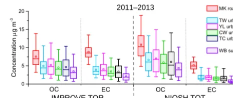
Figure 2.Three-year distributions of OC and EC concentrations by IMPROVE TOR and NIOSH TOT protocols for six sites in Hong Kong. The symbols in the boxplots represent the average (open circles), median (interior lines), 75th and the 25th percentile (box boundaries), and 95th and 5th percentile (whiskers).

laser transmittance and reflectance charring corrections; thus both TOT and TOR results can be obtained for each pro-tocol temperature program. As a result, four sets of analy-sis data are obtained and used for investigation of OC and EC determination dependency on analysis protocols in this study. The four sets of data are denoted as NIOSH TOT, NIOSH TOR, IMPROVE TOT, and IMPROVE TOR, with NIOSH and IMPROVE representing their respective tem-perature program and TOT and TOR representing the mean of charring correction based on laser transmittance and re-flectance, respectively. It should be noted that NIOSH TOT and IMPROVE TOR data represent data by the two proto-cols, while the other two sets of data are usually not re-ported in EC and OC analysis. The concentrations of water-soluble organic carbon (WSOC) and three sugar compounds (levoglucosan, mannosan, and galactosan) were available for 2013 WB samples from a separate project. WSOC concen-trations were measured by a TOC analyzer (Shimadzu TOC-VCPH, Japan) (Kuang et al., 2015). The sugars were

an-alyzed by high-performance anion-exchange chromatogra-phy (HPAEC) with a pulsed amperometric detection (PAD) method (Engling et al., 2006).

2.3 Quality assurance/quality control of OCEC data Since OC and EC are operationally defined and lack ref-erence materials, external calibration is only performed for TC on a biweekly basis using sucrose solutions (Wu et al., 2012). Duplication analysis covering 14 % of the to-tal samples was conducted for quality control purposes. TC by the two protocols (NIOSH and IMPROVE) agrees very well as evidenced by the unity regression slope (Fig. S2a, slope=0.99,R2=0.99) and sharp frequency distribution of NIOSH TC / IMPROVE TC ratios (Fig. S2b). Nevertheless, a small number of extreme data remain. The following criteria are used during the data processing to screen out the sus-picious data: 0.1<OC/EC<40; 0.5<TCNSH/TCIMP<2.

(4)

Table 1.Ambient mean concentrations (µg m−3) of OC and EC for six sites in Hong Kong by IMPROVE TOR and NIOSH TOT protocols.

Site Analysis Chow et Chow et Chow et Current study

protocol al. (2002)b al. (2006)b al. (2010)b

2001a 2005 2009 2011 2012 2013 3-year average

(Mean±one standard deviation)

MK IMPROVE OC 16.64 11.17 6.26 8.09±3.67 6.94±2.55 6.92±3.36 7.33±3.28

TOR EC 20.29 14.11 10.66 8.48±2.08 9.21±2.74 9.42±1.89 9.03±2.27

NIOSH OC 11.36±4.26 10.24±3.94 10.51±4.63 10.72±4.3

TOT EC 4.86±1.47 5.53±1.42 5.35±1.78 5.24±1.59

TW IMPROVE OC 8.69 6.93 4.38 5.44±3.35 4.5±2.4 4.86±3.47 4.94±3.14

TOR EC 5.37 6.25 3.76 4.24±1.81 3.62±1.99 4.01±1.71 3.97±1.84

NIOSH OC 7.37±4.05 6.1±3.33 6.79±4.46 6.77±4.01

TOT EC 1.95±0.93 1.76±0.91 1.91±0.87 1.88±0.9

YL TOR OC OC 7.23 4.83 5.62±3.56 4.77±3.02 4.92±4.05 5.16±3.63

TOR EC EC 6.19 3.48 4.56±2.48 3.69±1.8 3.92±1.87 4.08±2.1

TOT OC OC 7.92±4.69 6.33±3.94 6.88±4.92 7.12±4.62

TOT EC EC 1.89±0.9 1.79±0.91 1.95±1.12 1.88±0.98

CW IMPROVE OC 4.92±2.89 4.12±2.64 4.37±3.33 4.48±2.98

TOR EC 3.71±1.75 3.24±1.94 3.48±1.69 3.48±1.79

NIOSH OC 6.55±3.55 5.55±3.27 6.2±4.02 6.12±3.64

TOT EC 1.63±0.82 1.54±1.03 1.54±0.95 1.57±0.93

TC IMPROVE OC 5.13±3.69 4.17±2.68 4.27±4.23 4.53±3.63

TOR EC 3.65±2.3 3.1±1.71 3.37±2.14 3.38±2.08

NIOSH OC 6.88±4.74 5.48±3.37 6.03±5.39 6.15±4.63

TOT EC 1.53±0.91 1.55±0.87 1.46±0.91 1.51±0.89

WB IMPROVE OC 3.91±2.62 3.07±2 3.37±3.13 3.46±2.65

TOR EC 2.43±1.42 1.81±1.2 1.96±1.39 2.08±1.37

NIOSH OC 5.07±3.33 3.91±2.53 4.62±3.93 4.55±3.36

TOT EC 0.86±0.5 0.72±0.44 0.67±0.58 0.75±0.52

a_{November 2000–October 2001;}b_{studies using DRI2001 carbon analyzer.}

3 Results and discussion

3.1 Ambient PM2.5OC and EC concentrations

The 3-year distribution of OC and EC concentrations is shown in Fig. 2, where a clear spatial gradient can be seen from the roadside site to the urban sites and suburban site. OC and EC levels at the MK roadside site are a factor of 2 higher for both protocols compared to the urban sites. An-nual average concentrations and standard deviations for the five sites are listed in Table 1. Compared to samples collected at the MK and TW sites in November 2000–December 2001 (Chow et al., 2002), both OC and EC 3-year annual average concentrations observed in this study are lower by a factor of 1.4–2.3. At the TW site, TOR OC decreased from 8.69 to 4.94±3.14 µg m−3and TOR EC decreased from 5.37 to 3.97±1.84 µg m−3. The reduction is more pronounced at the MK roadside site, where TOR OC decreased from 16.64 to

7.33±3.28 µg m−3 and TOR EC decreased from 20.29 to 9.03±2.27 µg m−3(Chow et al., 2002).

3.2 NIOSH and IMPROVE comparison for OC and EC determination

(5)

(a)

(b)

(c)

60

50

40

30

20

10

0

AEC

IMP

μg cm

-2

60 50 40 30 20 10 0

AECNSH + OC4NSH μg cm-2

y=0.99x+0.12 R2=0.99 N=1398 WODR

1:1 line

50

40

30

20

10

0 ECIMP_TOR

μg cm

-2

25 20 15 10 5 0

ECNSH_TOT + OC4NSH μg cm-2

y=1.18x-0.60 R2=0.75 N=1398 WODR

2:1 line 50

40

30

20

10

0 ECIMP_TOR

μg cm

-2

25 20 15 10 5 0

ECNSH_TOT μg cm-2

y=2.05x+0.30 R2=0.76 N=1398 WODR

2:1 line

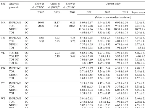
Figure 3.Comparison of different carbon fractions.(a)Relationship of IMPROVE apparent EC (AECIMP, sum of EC1IMPto EC3IMP)

and the sum of NIOSH apparent EC (AECNSH, sum of EC1NSHto EC6NSH)plus OC4NSH,(b)relationship of ECIMP_TOR(yaxis) and

ECNSH_TOT(xaxis), and(c)relationship of ECIMP_TOR(yaxis) and the sum of ECNSH_TOTand OC4NSH(xaxis). WODR stands for

weighed orthogonal distance regression.

two protocols. The carbon fraction evolved corresponding to the 870◦C step is classified as OC4 in the NIOSH protocol, while in IMPROVE this fraction is evolved as part of ap-parent EC (AEC), which is the sum of all the EC fractions before correcting for charred OC. Chow et al. (2001) found NIOSH OC4 can explain most of the EC difference in US samples between the two protocols, and this relationship has been further defined in a PRD study by our group (Eq. 1), where IMPROVE AEC is found to be equivalent to the sum of NIOSH OC4 and NIOSH AEC (Wu et al., 2012).

AECIMP=AECNSH+OC4NSH (1)

HK samples from the current study also confirm this re-lationship as shown in Fig. 3a (Slope=0.99). It should be noted that, due to the much longer step durations in the IMPROVE protocol, carbon evolved beyond 550◦C in IM-PROVE protocol does not simply map to OC evolved beyond the same temperature point in the NIOSH protocol (i.e., tem-perature step beyond 550◦_{C, which includes part of OC3 and}

OC4).

The reported IMPROVE TOR EC is the sum of carbon fractions evolved in the He–O2stage (AECIMP)minus PC as

measured by laser reflectance.

ECIMP_TOR=AECIMP−PCIMP_TOR (2)

Combining Eqs. (1) and (2), the IMPROVE TOR EC can be defined as

ECIMP_TOR=AECNSH+OC4NSH−PCIMP_TOR. (3)

Likewise, the reported NIOSH TOT EC is the sum of car-bon fractions evolved in the He–O2stage (AECNSH)minus

pyrolysis carbon by laser transmittance.

ECNSH_TOT=AECNSH−PCNSH_TOT (4)

As shown in Fig. 3b, the linear regression slope (2.05) of the scatterplot represents the average discrepancy be-tween ECIMP_TOR (yaxis) and ECNSH_TOT(x axis). As

em-bodied in Eqs. (3) and (4), the EC discrepancy can be at-tributed to two factors: OC4NSH (thermal effect) and the

difference in PC (optical method effect). Thermal effect refers to inter-protocol EC difference caused by tempera-ture step difference. The optical method effect is the inter-protocol EC difference introduced by the PC difference be-tween transmittance and reflectance charring correction. By adding OC4NSHto thexaxis (Fig. 3c), the effect of OC4NSH

between y (ECIMP_TOR) and x (OC4NSH+ECNSH_TOT) is

minimized as embodied in Eqs. (3) and (5), where the slope (1.18) primarily represents the optical method effect caused by the PC difference (PCIMP_TORvs. PCNSH_TOT).

ECNSH_TOT+OC4NSH= (5)

AECNSH+OC4NSH−PCNSH_TOT

The difference between the slopes in Fig. 3b (slope=2.05) and Fig. 3c (slope=1.18) indicates the contribution of the thermal effect to the EC discrepancy. By examining the rela-tive differences from unity in the two slopes (i.e., 0.18/1.05), it is estimated that 82.86 % of the EC difference by the two protocols in HK samples is attributed to the thermal effect (OC4NSH), and the rest (17.14 %) is due to the PC

moni-toring, arising from different optical methods used for the charring correction (laser transmittance or reflectance). The reduced R2 in Fig. 3b and c compared to Fig. 3a suggest the scatter of data points is due to the optical method effect (PC). The relative contribution of the two factors in the HK samples exhibits a seasonal dependency as shown in Fig. S3. In summer and fall, the optical method effect accounts for

∼12 % of the EC discrepancy, while in winter and spring the optical method effect contribution is 35 %. This is in part dic-tated by a lower proportion of OC4NSHfraction in these two

seasons as shown in Fig. S4, leading to an attenuated thermal effect.

(6)

10

8

6

4

2

0 ECIMP_TOR

/E

CNSH_TOT

μg cm

-2

10 8 6 4 2 0

PCIMP_TOT/PCIMP_TOR μg cm-2

y=0.00x+1.94 R2=0.00 N=700 WODR

1:1 line

Spring andwinter 10

8

6

4

2

0 ECIMP_TOR

/E

CNSH_TOT

μg cm

-2

10 8 6 4 2 0

PCNSH_TOT/PCNSH_TOR μg cm-2

y=0.73x+0.57 R2=0.12 N=508 WODR

1:1 line

Summer and fall 10

8

6

4

2

0 ECIMP_TOR

/E

CNSH_TOT

μg cm

-2

10 8 6 4 2 0

PCNSH_TOT/PCNSH_TOR μg cm-2

y=1.13x-0.56 R2=0.41 N=697 WODR

1:1 line

Spring andwinter

(a)

(b)

(c)

(Including effect of OC4NSH) (offset effect of OC4NSH) (Including effect of OC4NSH)

Figure 4. ECIMP_TOR-to-ECNSH_TOT discrepancy dependency on TOT/TOR charring correction. (a) ECIMP_TOR/ECNSH_TOT vs.

PCNSH_TOT/PCNSH_TORratio–ratio plot for summer and fall. (b) ECIMP_TOR/ECNSH_TOTvs. PCNSH_TOT/PCNSH_TOR ratio–ratio

plot for spring and winter.(c)ECIMP_TOR/ECNSH_TOTvs. PCIMPTOT/PCIMP_TORratio–ratio plot for spring and winter.

8

6

4

2

0

EC

IM

P_T

O

R

/EC

NSH_T

O

T

3.0 2.5 2.0 1.5 1.0 0.5 0.0

K+/ECNSH_TOT

y=2.74x+1.36

R2=0.39 N=1205 WODR

3:1 line

8

6

4

2

0

EC

IM

P_TOR

/(EC

NSH_TOT

+OC4

NSH

)

3.0 2.5 2.0 1.5 1.0 0.5 0.0

K+/ECNSH_TOT

y=‐0.44x+1.05

R2=0.02 N=1205 WODR

3:1 line

Including effect of OC4NSH

offset effect of OC4NSH

(a)

(b)

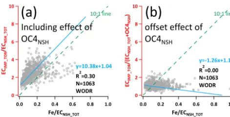
Figure 5. ECIMP_TOR-to-ECNSH_TOT discrepancy

depen-dency on K+/ECNSH_TOT ratio (biomass burning effect).

(a) ECIMP_TOR/ECNSH_TOT vs. K+/ECNSH_TOT ratio–

ratio plot. (b) ECIMP_TOR/(ECNSH_TOT+OC4NSH) vs.

K+/ECNSH_TOTratio–ratio plot.

It is found that the ratio of ECIMP_TOR/ECNSH_TOT shows

a dependency on PCNSH_TOT/PCNSH_TOR(R2=0.12–0.41),

and the degree of correlation varies by season (Fig. 4a and b). This result agrees well with the higher optical method ef-fect contribution during spring and winter shown in Fig. S3 and discussed above. In contrast, ECIMP_TOR/ECNSH_TOT

is insensitive to PCIMP_TOT/PCIMP_TOR (R2=0) as shown

in Fig. 4c. This selective dependency suggests the optical method effect contribution to EC dependency is distinctly sensitive to the degree of charring formed during the OC4NSH

stage. Since PCNSH contains char formed in the OC4NSH

stage while PCIMPdoes not, OC4NSHis the major difference

between potential sources of PCIMPand PCNSHdifference.

3.2.1 Effect of biomass burning on OC and EC determination between IMPROVE and NIOSH Other potential factors affecting EC discrepancy were also examined. Cheng et al. (2011a) found in Beijing samples that biomass burning can influence the EC discrepancy. Here we use a normalized abundance of K+as an indicator to

exam-ine the impact of biomass burning on the EC discrepancy. Figure S5a is the same as Fig. 3b but color coded with the K+/ECNSH_TOTratio to reflect the influence from biomass

burning. It reveals a pattern associated with the ECIMP_TOR

-to-ECNSH_TOT ratio. To verify this relationship, regressions

on the lowest and highest 10 % of K+/ECNSH_TOT

ra-tios are shown in Fig. S6b and S6c, respectively. The data from the highest 10 % of K+/ECNSH_TOTratios have a

sig-nificantly higher regression slope (slope=3.19, Fig. S5c) than the data from the lowest 10 % of K+/ECNSH_TOT

ra-tios (slope=1.48, Fig. S5b), implying the EC discrepancy depends on the K+/ECNSH_TOT ratio. To further

distin-guish whether the K+/ECNSH_TOTeffect is associated with

OC4NSH (thermal effect) or the difference in PC (optical

method effect), OC4NSH is added to the x axis as shown

in Fig. S5d–f. By adding OC4NSH to the x axis, any

dis-crepancy between y andx can be attributed to the optical method effect alone. The slopes of samples from the high-est 10 % of K+/ECNSH_TOTratios (1.20, Fig. S5e) and

sam-ples from the lowest 10 % of K+/ECNSH_TOT ratios (1.27,

Fig. S5f) are very close to the slope using all samples (1.23, Fig. S5d), implying that the optical method effect is not sen-sitive to the K+/ECNSH_TOTratio. Consequently, the EC

dis-crepancy dependence on the K+/ECNSH_TOT ratio is very

likely associated with OC4NSH (thermal effect). Since the

intercepts in Fig. S5 are relatively small and their slopes can be represented by ratios, we use ratio–ratio plots to verify the relationship of K+/ECNSH_TOT to OC4NSH. As

shown in Fig. 5a, when the K+_/_EC

NSH_TOTratio goes up,

a larger EC discrepancy is observed; while adding OC4NSH

to they axis (offsetting the contribution from OC4NSH)as

shown in Fig. 5b, this relationship no longer holds. The OC4NSH fraction, as represented by the relative abundance

of OC4NSH in samples (OC4NSH/TC), exhibits a

depen-dency on the K+/ECNSH_TOTratio as illustrated in the

his-tograms of Fig. S6. An independent t test (Table S2) was performed, finding the average OC4NSH/TC ratio of

sam-ples from the highest 10 % of K+/ECNSH_TOTratios (0.27,

(7)

aver-10

8

6

4

2

0

EC

IM

P_T

O

R

/E

CNS

H

_

TO

T

1.0 0.8 0.6 0.4 0.2 0.0

Fe/ECNSH_TOT

y=10.38x+1.04

R2=0.30 N=1063 WODR

10:1 line

10

8

6

4

2

0

EC

IM

P_T

O

R

/(

EC

NS

H

_

TO

T

+O

C4

NSH

)

1.0 0.8 0.6 0.4 0.2 0.0

Fe/ECNSH_TOT

y=‐1.26x+1.12

R2=0.00 N=1063 WODR

10:1 line

Including effect of OC4NSH

offset effect of OC4NSH

(a)

(b)

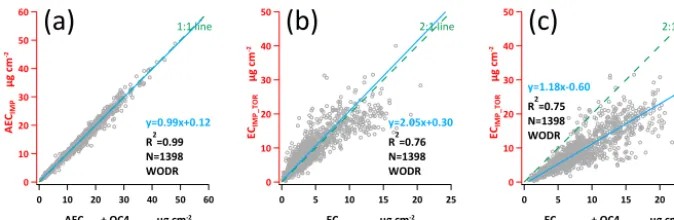
Figure 6. EC_{IMP_TOR}-to-EC_{NSH_TOT} discrepancy

de-pendency on Fe/ECNSH_TOT ratio (metal oxide effect).

(a)ECIMP_TOR/ECNSH_TOTvs. Fe/ECNSH_TOTratio–ratio plot. (b) ECIMP_TOR/(ECNSH_TOT+OC4NSH) vs. Fe/ECNSH_TOT

ratio–ratio plot.

age OC4NSH/TC ratio of samples from the lowest 10 % of

K+/ECNSH_TOTratios, which reveals that the OC4NSH

frac-tion and K+/ECNSH_TOTratio are positively correlated. As

discussed before, the OC4NSHfraction can affect the EC

dis-crepancy, which is the reason that biomass burning can influ-ence the EC discrepancy.

3.2.2 Effect of metal oxides on OC and EC

determination between IMPROVE and NIOSH A suite of laboratory studies have revealed the presence of metal oxides in aerosol samples can alter the EC/OC ratio, by either lowing the EC oxidation temperature or enhancing OC charring (Murphy et al., 1981; Wang et al., 2010; Bladt et al., 2014). As a result, the distribution of carbon fractions is impacted during the analysis, affecting the inter-protocol EC discrepancy. As shown in Figs. 6a and S7, the EC dis-crepancy positively correlates with normalized Fe abundance (Fe/ECNSH_TOTratio), suggesting that a higher fraction of

metal oxide can increase the EC divergence across the two protocols. If OC4NSHis added to cancel out the discrepancy

contribution from the thermal effect (Figs. 6b and S7), the discrepancy due to the optical method effect alone shows no dependency on Fe abundance. Similar dependency is also found in other metal oxides like Al as shown in Fig. S8. These results imply that metal-oxide-induced EC divergence is mainly associated with the OC4NSHfraction.

3.3 Comparison of IMPROVE TOR EC reconstruction approaches for Hong Kong samples

3.3.1 Description of two reconstruction methods It is of great interest to determine the best estimation for ECIMP_TOR when only NIOSH TOT analysis is available.

This study provides an opportunity to examine different em-pirical reconstruction approaches for ECIMP_TOR using the

ECNSH_TOTdata. In total, four approaches are investigated;

two of them are discussed below, and the other two are

discussed in the Supplement. The first method is direct re-gression (M1), which applies the relationship obtained from Fig. S9 to reconstruct ECIMP_TOR:

M1: ECIMP_TOR=a×ECNSH_TOT+b (6)

Then, reconstructed OCIMP_TOR can be obtained by

sub-tracting reconstructed ECIMP_TORfrom TCNSH:

reconstructed OCIMP_TOR= (7)

TCNSH−reconstructed ECIMP_TOR.

Further reconstruction methods may deconstruct ECIMP_TOR into several terms based on analysis

princi-ples and apply regression only on the unknown terms. Since only a partial regression is involved, theoretically, this approach can provide more accurate reconstruction results. Relationships found in Sect. 3.2 can also be used to refine the reconstruction.

The second approach (M2) employs partial regression. In Eq. (3), PCIMP_TOR is the only unknown term on the

right-hand side. As shown in Fig. S10, PCIMP_TOR is well

corre-lated with PCNSH_TOR, which is known from NIOSH

analy-sis. Therefore, Eq. (3) can be approximated as

M2: ECIMP_TOR= (8)

AECNSH+OC4NSH−(a×PCNSH_TOR+b).

M2 can be further improved if chemical composition data are available. As discussed above, the abundance of K+ and Fe can affect EC discrepancy. To reflect the contribu-tions from these factors, PCNSH_TOR, K+, and Fe are

in-cluded to approximate PCIMP_TORby multiple linear

regres-sion (MLR), then Eq. (3) can be rewritten as

M2−1:ECIMP_TOR=AECNSH+OC4NSH (9) −(a1×PCNSH_TOR+a2×K++a3×Fe+b). a1,a2, anda3are MLR coefficients. K+is measured by ion

chromatography, and Fe is detected by X-ray fluorescence. An alternative reconstruction method (M3) is discussed in the Supplement. In brief, M3 is based on the linear relation-ship between (PCNSH_TOT–PCNSH_TOR) and (PCNSH_TOT–

PCIMP_TOR)for reconstruction.

3.3.2 Reconstruction of 2013 OC and EC using parameters from 2011–2012 data

(8)

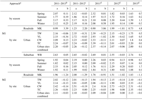
Table 2.Regression parameters for OC and EC reconstruction equations.

Approacha 2011–2013b 2011–2012c 2011d 2012d 2013d

a b a b a b a b a b

by season

Spring 2.07 0.11 2.12 −0.03 2.32 0.01 1.82 0.03 1.63 0.74

Summer 1.77 0.19 1.86 0.14 1.97 0.13 1.72 0.16 1.63 0.24

Fall 2.17 0.33 2.17 0.21 2.10 0.08 2.20 0.44 1.59 1.37

Winter 2.12 0.25 2.19 0.16 2.08 0.58 1.95 0.14 1.99 0.39

by site

Roadside MK 0.99 3.39 1.23 2.20 0.90 3.86 1.99 −1.81 0.73 4.87

M1

Urban

TW 2.16 −0.06 2.35 −0.31 2.39 −0.23 2.15 −0.23 1.75 0.54

YL 2.33 −0.34 2.72 −0.83 2.93 −1.02 2.30 −0.42 1.65 0.55

CW 2.09 0.13 2.23 −0.02 2.33 −0.11 2.11 0.07 1.8 0.44

TC 2.24 −0.07 2.24 −0.09 2.39 −0.11 2.01 −0.03 2.20 0.02

Urban sites 2.20 −0.05 2.26 −0.12 2.37 −0.14 2.07 −0.06 2.00 0.16

combined

Suburban WB 2.63 0.05 2.65 −0.02 2.69 0.01 2.55 −0.03 2.74 0.10

by season

Spring 1.92 0.04 2.19 0.00 2.26 0.03 0.94 0.13 0.98 0.34

Summer 1.82 0.02 2.15 0.00 2.09 −0.02 2.15 0.07 1.14 0.04

Fall 2.33 0.16 2.05 0.12 1.76 0.11 2.29 0.20 0.03 1.72

Winter 1.92 0.11 1.99 0.02 1.84 0.31 1.80 0.02 1.88 0.18

by site

Roadside MK 1.96 −1.24 2.00 −1.29 1.78 −0.91 1.51 −1.02 1.83 −1.11

M2

Urban

TW 2.02 −0.12 2.01 −0.13 1.94 −0.13 2.15 −0.14 2.10 −0.10

YL 2.14 −0.13 2.01 −0.05 2.08 −0.11 1.90 0.03 2.33 −0.20

CW 2.42 −0.14 2.51 −0.19 2.4 0.16 2.73 −0.23 2.31 −0.10

TC 2.26 −0.01 2.23 0.00 2.25 −0.03 1.98 0.08 2.35 −0.02

Urban sites 2.11 −0.03 2.10 −0.03 2.09 −0.04 2.09 0.00 2.13 −0.03

combined

Suburban WB 2.65 0.11 2.74 0.07 2.86 0.03 2.47 0.14 2.70 0.14

a_{The two reconstruction method equations are}_M1_:_EC

IMP_TOR=a×ECNSH_TOT+b;M2:ECIMP_TOR=AECNSH+OC4NSH−(a×PCNSH_TOR+b).

b_{Regression parameters are derived from 2011–2013 data.}c_{Regression parameters are derived from 2011–2012 data.}d_{Regression parameters are derived from a single} year’s data.

are considered for parameterization: scenario 1, seasonal spe-cific parameters for each season with samples from all sites; scenario 2, site-specific parameters for all samples from a site or combined sites with a similar site characteristic. De-tailed parameters are summarized in Table 2. These param-eters are then applied to NIOSH data in 2013, and recon-structed ECIMP_TOR and OCIMP_TORconcentrations are

cal-culated and compared with measured 2013 ECIMP_TOR and

OCIMP_TOR to evaluate the performance of OC and EC

re-construction by the two scenarios. Since two scenarios are considered in each reconstruction method, there are four combinations of reconstruction results for M1 and M2.

Reconstructed EC by M1 is compared with measured EC in Fig. 7a and b. TheR2of the season-specific (Fig. 7a) and site-specific reconstruction (Fig. 7b) are comparable with each other. Reconstructed EC is also compared with mea-sured EC using histograms as shown in Fig. S15. The mean concentration by site-specific reconstruction agrees better than the season-specific reconstruction. The frequency dis-tribution of the relative difference of reconstructed vs.

mea-sured EC exhibits a similar distribution between the season-and site-specific reconstructions (Fig. S16). OC tion by M1 is shown in Fig. 8a and b, revealing reconstruc-tion by site-specific parameters can increase theR2, with a tradeoff of higher average bias (slope=1.14). The seasonal or site-specific parameters yield similar reconstructed OC distributions as shown in Figs. S17 and S18. The OC/EC ratios reconstructed by M1 are overestimated by a factor of 2 as shown by the slopes in Fig. 9. The reconstructed OC/EC distribution is significantly broader than the mea-sured OC/EC ratios as shown in Figs. S19 and S20. This is an expected result of reconstructed OC and EC inherently having bias of opposite signs (i.e., if reconstructed OC is bi-ased higher, then reconstructed EC would be bibi-ased lower), amplifying the bias in the ratio quantity.

Results of ECIMP_TOR reconstruction by M2 are shown

(9)

supe-30 25 20 15 10 5 0 Re co nstr uc te d EC IMP _TOR μg m -3 30 25 20 15 10 5 0

ECIMP_TOR μg m-3

y=1.06x-0.15 R2=0.86 N=314 WODR 1:1 line M1 season-specific parameter 30 25 20 15 10 5 0 Reco nst ru ct ed E

CIMP_

TOR μg m -3 30 25 20 15 10 5 0

y=0.90x+0.22 R2=0.93 N=313 WODR

1:1 line M2

season parameter

30 25 20 15 10 5 0 Re co nstructed EC IMP _TOR μg m -3 30 25 20 15 10 5 0

ECIMP_TOR μg m-3

y=1.08x-0.18 R2=0.85 N=314 WODR

1:1 line M1

si parameter

30 25 20 15 10 5 0 Reco nst ru ct ed E

CIMP_

TOR μg m -3 30 25 20 15 10 5 0

y=0.95x+0.10 R2=0.96 N=313 WODR

1:1 line M2

si parameter

(c)

(d)

(a)

(b)

Roadside Urban Suburban Roadside Urban Suburban Roadside Urban Suburban Roadside Urban Suburban

Figure 7.Comparison of reconstructed ECIMP_TORand

measure-ment EC_{IMP_TOR} in the year 2013. (a) Regression by

season-specific parameters using M1.(b) Regression by site-specific

pa-rameters using M1.(c)Regression by season-specific parameters

using M2.(d)Regression by site-specific parameters using M2.

rior performance of M2 by site-specific parameters is also evidenced by the sharpened distribution peak around zero for the relative difference of measured and reconstructed EC (Fig. S16d). OC reconstruction by M2 using site-specific pa-rameters (Fig. 8d) yields a higherR2than the season-specific scenario (Fig. 8c). The OC relative difference distribution is sharpest in the site-specific-parameters scenario as shown in Fig. S18d. The OC/EC ratios reconstructed by M2 are un-derestimated by 22 to 72 % as shown in Fig. 9, with a lowR2

ranging from 0.3 to 0.46. The OC/EC bias is also evidenced by significantly different histograms between the distinctly sharper peak of the reconstructed OC/EC compared with measured OC/EC (Fig. S19c and d).

From the comparisons shown above, it is obvious that the M2 site-specific-parameters scenario can provide the best performance in OC and EC reconstruction, evidenced by regression slopes being closest to unity and the sharpest frequency distribution histograms of OC or EC differences between reconstructed and measured values. However, the OC/EC ratio is not well reproduced by the two methods; it is overestimated and underestimated by M1 and M2, respec-tively.

To investigate the stability of various parameters used in the two reconstruction scenarios, we also calculate recon-struction parameters for individual years from 2011 to 2013 as well as for the entire 3-year dataset as listed in Table 2. The reconstruction parameters are of similar values between

30 25 20 15 10 5 0 Re co nst ruc te d O CIMP _TOR μg m -3 30 25 20 15 10 5 0

OCIMP_TOR μg m-3 y=1.08x-0.35

R2=0.83

N=313 WODR 1:1 line M1 season-specific er 30 25 20 15 10 5 0 Re co nst ruc te d O CIMP _TOR μg m -3 30 25 20 15 10 5 0

OCIMP_TOR μg m-3 y=1.09x-0.13

R2=0.93

N=313 WODR 1:1 line M2 season-specific er 30 25 20 15 10 5 0 Re co nst ruc te d O CIMP _TOR μg m -3 30 25 20 15 10 5 0

OCIMP_TOR μg m-3 y=1.14x-0.52

R2=0.91

N=313 WODR 1:1 line M1 site-specific 30 25 20 15 10 5 0 Re co nst ruc te d O CIMP _TOR μg m -3 30 25 20 15 10 5 0

OCIMP_TOR μg m-3 y=1.02x+0.00

R2=0.96

N=313 WODR 1:1 line M2 site-specific parameter

(c)

(d)

(a)

(b)

Figure 8.Reconstruction of OCIMP_TORcalculated using Eq. (7).

(a)Reconstruction by season-specific parameters using M1.(b)

Re-construction by site-specific parameters using M1.(c)

Reconstruc-tion by season-specific parameters using M2.(d)Reconstruction by

site-specific parameters using M2.

10 8 6 4 2 0 Reco nstruc ted OC/EC IM P_TOR 10 8 6 4 2 0 OC/ECIMP_TOR y=2.12x‐1.10

R2=0.52 N=313 WODR 1:1 line M1 10 8 6 4 2 0 Reco nstruc ted OC/EC IM P_TOR 10 8 6 4 2 0 OC/ECIMP_TOR y=0.28x+0.82

R2=0.30 N=313 WODR 1:1 line M2 10 8 6 4 2 0 Reco nstruc ted OC/EC IM P_TOR 10 8 6 4 2 0 OC/ECIMP_TOR y=2.11x‐1.08

R2=0.51 N=313 WODR 1:1 line M1 10 8 6 4 2 0 Reco nstruc ted OC/EC IM P_TOR 10 8 6 4 2 0 OC/ECIMP_TOR y=0.78x+0.25

R2=0.46 N=313 WODR 1:1 line M2

(c)

(d)

(a)

(b)

Figure 9.Reconstruction results of OC/ECIMP_TOR.(a)

Recon-struction by season-specific parameters using M1.(b)

Reconstruc-tion by site-specific parameters using M1.(c)Reconstruction by

season-specific parameters using M2.(d) Reconstruction by

(10)

(b)

(c)

(a)

60 40 20 0 Fr eq ue nc y 12 10 8 6 4 2 0

SOCIMP_TOR μg m-3

100 80 60 40 20 0 Cu m ula ti ve dis trib u ti on (% )

mean ± 1 SD

2.66 ± 2.07

mode ± 1σ

Log: 1.10 ± 0.73 N=1313

Lognormal

Cumulative

50 40 30 20 10 0 Fr eq ue nc y 12 10 8 6 4 2 0

SOCNSH_TOT μg m-3

100 80 60 40 20 0 Cu m ula ti ve dis trib u ti on (% )

mean ± 1 SD

4.70 ± 3.35

mode ± 1σ

Log: 1.86 ± 0.83 N=1361

Lognormal

Cumulative

20 15 10 5 0 SO

CNSH_

TO T μg m -3 20 15 10 5 0

y=1.67x+0.11

R2=0.61

N=1301 WODR

1:1 line

Figure 10.Comparison of SOC by NIOSH and IMPROVE.(a)SOC estimation from NIOSH TOT data.(b)SOC estimation from IMPROVE

TOR data.(c)The relationship between SOC_{NSH_TOT}and SOC_{IMP_TOR}.

100 80 60 40 20 0 Freq uency 12 10 8 6 4 2 0

M1

Mean ± 1 SD 3.53 ± 2.88

2.66 ± 2.07

Mode ± 1 N=1234 N=1313 100 80 60 40 20 0 Freq uency 12 10 8 6 4 2 0

SOCIMP_TOR μg m-3 Mean ± 1 SD 1.99 ± 1.68

2.66 ± 2.07

Mode ± 1 N=1282 N=1313

(a)

(c)

20 15 10 5 0 Rec onstru c ted SO

CIMP_TO

R μg m -3 20 15 10 5 0

y=1.35x-0.29

R2=0.54

N=1182 WODR 1:1 line M1 20 15 10 5 0 Rec onstru c ted SO

CIMP_TO

R μg m -3 20 15 10 5 0

y=0.76x+0.02

R2=0.46

N=1240 WODR 1:1 line M2 M2

(b)

(d)

Figure 11.Histogram comparison of original SOCIMP_TOR(in red)

with SOCIMP_TOR(in blue) reconstructed by M1(a)and by M2(c).

Scatterplot comparison of original SOCIMP_TOR (inx axis) with

SOCIMP_TOR(inyaxis) reconstructed by M1(b)and by M2(d).

years, implying these methods are robust for future recon-struction applications. The implementation of M1 to all ur-ban site data (without site or seasonal specificity) yields the following equation, and this equation is recommended for ur-ban site data conversion.

M1(urban data): ECIMP_TOR= (10)

2.20×ECNSH_TOT−0.05

For a heavily trafficked roadside environment, the recom-mended slope and intercept are 0.99 and 3.39, respectively. For suburban environments with light EC loadings, the rec-ommended values are 2.63 for slope and−0.05 for intercept.

The M2 site-specific parameters exhibit weaker site de-pendence than the M1 method, making M2 more suitable for expanding its application in other regions. As a result, M2 site-specific parameters obtained from the 3-year dataset are recommended for future reconstruction applications in Hong Kong (Table 2). The equation for urban environments is shown below:

M2(urban data): ECIMP_TOR= (11)

AECNSH+OC4NSH−(2.11×PCNSH_TOR−0.03).

We note that the AECNSH, OC4NSH, and PCNSH_TORinputs

required in M2 are not always available for data users, as they are typically not reported by analysis laboratories.

Similarly, M2−1 site-specific parameters obtained from the 3-year dataset are recommended for future reconstruction applications in Hong Kong if K+and Fe data are available (Table S4). The equation for urban environments is given be-low:

M2−1(urban data): ECIMP_TOR= (12)

AECNSH+OC4NSH−(0.94×PCNSH_TOR+1.60 ×K++1.47×Fe+0.00).

Monthly variations of measured and reconstructed IM-PROVE TOR EC and OC (M2, site-specific parameters) are shown in Fig. S21, clearly showing the reconstructed OC and EC data can reproduce the monthly trend quite well as com-pared with the measured data. This demonstrates that the re-construction equations can provide a means to establish tem-poral trends for OCEC data produced using different analysis protocols.

3.4 Implications for secondary OC (SOC) estimation The EC tracer method (Turpin and Huntzicker, 1995) is a widely used approach for SOC estimation since it only re-quires measured OC and EC as input:

SOC=OCtotal−

_OC

EC

pri

(11)

where (OC/EC)pri is the OC/EC ratio in freshly

emit-ted combustion aerosols, OCtotal and EC are from the

mea-surements, and OCnon-comb is the OC fraction from

non-combustion sources (i.e., biogenic emissions). Since the OCnon-comb is usually small, it is considered as zero to

sim-plify the calculation in our study. The key to the EC tracer method is to estimate a proper (OC/EC)pri. Our previous

study proved that the minimum R squared method (MRS) is more accurate than the conventional subset percentile or min-imum OC/EC ratio approaches (Wu and Yu, 2016). There-fore, MRS is employed for SOC calculation in this study. In this section, two aspects are discussed regarding SOC esti-mation: (1) variability of OC and EC by different protocols and the impacts on SOC estimation and (2) the usability of reconstructed ECIMP_TOR and OCIMP_TOR for SOC

estima-tion.

Since the proportion of different primary emission sources is expected to vary by season, (OC/EC)pri is calculated

by MRS for each season (Table S3) using all 3 years of data (2011–2013). As shown in Fig. 10, SOC by NIOSH TOT (mean concentration: 4.70 µg m−3)is higher than by the IMPROVE TOR protocol (mean concentration: 2.66 µg m−3). On average, SOCNSH_TOTis 1.67 times higher

than SOCIMP_TOR as suggested by the regression slope in

Fig. 10c. Although the absolute SOC concentrations by the two protocols are quite divergent, theR2(0.61) suggests that the two SOCs are moderately correlated. WSOC has been recognized as a good indicator of SOC formation (Sullivan et al., 2004), but WSOC contribution from primary emission is not negligible (Graham et al., 2002). Instead of using WSOC directly, we use secondary WSOC (SWSOC) as an indicator to verify the SOC results. SWSOC can be calculated from the following equation:

SWSOC=WSOC−sugars×

_WSOC

sugars

pri

. (14)

In Eq. (14), sugars – which include levoglucosan, man-nosan, and galactosan – are used as a tracer to derive SWSOC based on the primary ratio (5.28, Fig. S22) ob-tained from a biomass burning source profile measured in the PRD region (Lin et al., 2010). The relationship between SWSOC and SOC is examined in Fig. S23 for the WB site where sugars and WSOC data are available. SWSOC ac-counts for 61 % of SOCNSH_TOT, which is comparable with

the WSOC/SOCNSH_TOT ratio observed in Beijing (50–

70 %) by Cheng et al. (2011b). The SWSOC-to-SOCIMP_TOR

regression slope is close to unity (0.92), implying that SOC by IMPROVE TOR could be underestimated. SOC by both SOCNSH_TOTand SOCIMP_TOR is well correlated with

SWSOC, confirming the significant contribution of WSOC to SOC in this region. SOCNSH_TOTexhibits a higher

correla-tion (R2=0.92) with WSOC than SOCIMP_TOR(R2=0.86),

which is in good agreement with the study in Beijing (Cheng et al., 2011b), suggesting that NIOSH TOT might be more reasonable for SOC estimation.

The usability of reconstructed ECIMP_TORand OCIMP_TOR

(using M1 and M2) for SOC estimation is investigated. Re-sults of M2−1 and M3 are discussed in Supplement. To ac-count for the temporal variations of (OC/EC)pri, seasonal

(OC/EC)pri values are calculated using OC and EC

recon-structed by M1 and M2 (Table S3). These (OC/EC)pri

val-ues are then subject to SOC estimation following Eq. (13). It is very clear that the frequency distribution of recon-structed SOCs deviates from the SOC derived from mea-sured OC and EC (Fig. 11). The SOC by M1 is higher than the original SOC, evidenced by average concentrations (3.53 vs. 2.66 µg m−3)and also confirmed by the regression slope (1.35). On the other hand, SOC by M2 is underestimated by 30–40 %. The moderateR2(Fig. 11d) also suggests the SOC by reconstructed ECIMP_TOR and OCIMP_TOR is poorly

cor-related with SOC by measured ECIMP_TOR and OCIMP_TOR.

The significant bias and moderate correlations suggest that reconstructed ECIMP_TORand OCIMP_TORare not suitable for

SOC estimation.

4 Conclusions

In this study, we use a large dataset that has good temporal (3 years) and spatial coverage (roadside, urban, rural) in Hong Kong to investigate the OC and EC determination discrep-ancy between NIOSH TOT and IMPROVE TOR protocols. NIOSH TOT reported lower EC (higher OC) than IMPROVE TOR. The divergence between the two protocols is attributed to two effects: thermal effect and optical method effect. The thermal effect is due to the higher PIMT in NIOSH (870◦C) than IMPROVE (550◦_{C) and the allocation of the OC4}

NSH

fraction. The optical method effect is a result of different laser signals used by the two protocols (laser transmittance by NIOSH vs. laser reflectance by IMPROVE).

The equivalence between AECIMP and sum of OC4NSH

and AECNSH is confirmed in the current study, and by

off-setting the discrepancy from the thermal effect (OC4NSH),

the contribution from laser correction can be quantified. It is found that on average the thermal effect accounted for 83 % of the EC disagreement, while 17 % is attributed to the opti-cal method effect. The contribution of the two effects exhibits a clear seasonal dependency, with a more pronounced optical method effect in spring and winter (∼35 %).

The intensity of biomass burning influence can af-fect EC divergence between the two protocols. Sam-ples influenced by biomass burning (evidenced by higher K+_/_EC

NSH_TOTratio) come with higher OC4NSHabundance

(higher OC4NSH/TC ratio), leading to larger EC divergence

between the two protocols. The abundance of metal oxide in samples can also affect EC discrepancy, with a larger EC difference observed when a higher fraction of metal oxide is present in the ambient samples.

(12)

parameterization scenarios are considered, including season-specific parameters and site-season-specific parameters. The imple-mentation of M1 to all urban sites (without considering sea-sonal specificity) yields the following equation:

M1(urban data): ECIMP_TOR=2.20×ECNSH_TOT−0.05.

Considering site specificity yields slightly better reconstruc-tion performance, with the site-specific slope value varying from 2.16 to 2.33 for the urban sites. The suburban site produces a higher slope value (2.63), while the roadside (MK) data produce a noticeably lower slope value (0.99). Hence, roadside samples (i.e., typically significant EC load-ings) need to be processed separately and applied its own site-specific parameters for reconstruction when using the M1 equation. The comparisons show that M2−1 with site-specific parameters provides the best reconstruction results, and the regression parameters are given in Tables 2 and S4.

SOC estimation using OC and EC by the two protocols is compared. Based on the SWSOC-to-SOC ratio and corre-lation coefficients, it is found that SOC concentrations de-rived from NIOSH TOT are likely more reasonable than those from IMPROVE TOR. The reconstructed ECIMP_TOR

and OCIMP_TORfor SOC estimation are shown to be

unsuit-able due to the poor reconstruction of the OC/EC ratio.

5 Recommendations for applying OCEC reconstruction

It should be noted that the conversion equations established in this work are based on the fact that all OCEC data analy-sis was done by the same analyzer. Other instrument-specific parameters might influence the regression if multiple instru-ments are used in obtaining the OCEC data. For example, temperature offset has been found to vary by instrument in different labs (Panteliadis et al., 2015). Oven soiling and ag-ing have also been found to have an optical influence that in-troduces uncertainties in the results (Chiappini et al., 2014).

Four reconstruction approaches are proposed in this study; the selection of which to use depends on the degree of avail-ability of the dataset. If the dataset has only OC and EC con-centrations and no detailed carbon fraction information, M1 is preferred. If the dataset also comes with carbon fraction information, M2 and M3 are suggested. If chemical specia-tion data are available, such as K+ and Fe, M2−1 is rec-ommended to minimize the effect from biomass burning and metal oxides.

6 Data availability

OC, EC, inorganic ions and elements data used in this study are available from Hong Kong Environmental Protection De-partment ([email protected]).

The Supplement related to this article is available online at doi:10.5194/amt-9-4547-2016-supplement.

Acknowledgements. This project was partially supported by the Hong Kong Environment Protection Department (HKEPD) (AS 10-231, 11-03973, and 12-04384). We thank HKEPD for making available the data for this work. We are indebted to Peter Louie

for his relentless efforts in pushing for the best possible PM2.5

speciation measurements in Hong Kong.

Edited by: W. Maenhaut

Reviewed by: two anonymous referees

References

Birch, M. E. and Cary, R. A.: Elemental carbon-based method for monitoring occupational exposures to particulate diesel exhaust, Aerosol. Sci. Technol., 25, 221–241, 1996.

Bladt, H., Ivleva, N. P., and Niessner, R.: Internally mixed mul-ticomponent soot: Impact of different salts on soot structure and thermo-chemical properties, J. Aerosol. Sci., 70, 26–35, doi:10.1016/j.jaerosci.2013.11.007, 2014.

Boggs, P. T., Donaldson, J. R., and Schnabel, R. B.: Algorithm 676: ODRPACK: software for weighted orthogonal distance regres-sion, ACM T. Math. Software., 15, 348–364, 1989.

Bond, T. C., Zarzycki, C., Flanner, M. G., and Koch, D. M.: Quan-tifying immediate radiative forcing by black carbon and organic matter with the Specific Forcing Pulse, Atmos. Chem. Phys., 11, 1505–1525, doi:10.5194/acp-11-1505-2011, 2011.

Cheng, Y., Duan, F.-K., He, K.-B., Zheng, M., Du, Z.-Y., Ma, Y.-L., and Tan, J.-H.: Intercomparison of thermal–optical methods for the determination of organic and elemental carbon: influences of aerosol composition and implications, Environ. Sci. Technol., 45, 10117–10123, doi:10.1021/es202649g, 2011a.

Cheng, Y., He, K.-B., Duan, F.-K., Zheng, M., Du, Z.-Y., Ma, Y.-L., and Tan, J.-H.: Ambient organic carbon to ele-mental carbon ratios: Influences of the measurement meth-ods and implications, Atmos. Environ., 45, 2060–2066, doi:10.1016/j.atmosenv.2011.01.064, 2011b.

Cheng, Y., He, K.-B., Duan, F.-K., Du, Z.-Y., Zheng, M., and Ma, Y.-L.: Ambient organic carbon to elemental carbon ra-tios: Influence of the thermal–optical temperature protocol and implications, Sci. Total Environ., 468–469, 1103-1111, doi:10.1016/j.scitotenv.2013.08.084, 2014.

Chiappini, L., Verlhac, S., Aujay, R., Maenhaut, W., Putaud, J. P., Sciare, J., Jaffrezo, J. L., Liousse, C., Galy-Lacaux, C., Alleman, L. Y., Panteliadis, P., Leoz, E., and Favez, O.: Clues for a stan-dardised thermal-optical protocol for the assessment of organic and elemental carbon within ambient air particulate matter, At-mos. Meas. Tech., 7, 1649–1661, doi:10.5194/amt-7-1649-2014, 2014.

(13)

Chow, J. C., Watson, J. G., Crow, D., Lowenthal, D. H., and Merrifield, T.: Comparison of IMPROVE and NIOSH carbon measurements, Aerosol. Sci. Technol., 34, 23–34, doi:10.1080/027868201300081923, 2001.

Chow, J. C., Watson, J. G., Kohl, S., Gonzi, M., Chen, L.-W. A., and Chai, W.: Measurements and validation for the twelve month par-ticulate matter study in Hong Kong, Hong Kong Environmental Protection Department, Hong Kong, 2002.

Chow, J. C., Watson, J. G., Chen, L. W. A., Arnott, W. P., and Moosmuller, H.: Equivalence of elemental carbon by ther-mal/optical reflectance and transmittance with different tem-perature protocols, Environ. Sci. Technol., 38, 4414–4422, doi:10.1021/Es034936u, 2004.

Chow, J. C., Watson, J. G., Kohl, S., Gonzi, M., Chen, L.-W. A., and Chai, W.: Measurements and validation for the twelve month par-ticulate matter study in Hong Kong, Hong Kong Environmental Protection Department, Hong Kong, 2006.

Chow, J. C., Watson, J. G., Kohl, S., Chen, L.-W. A., and Chai, W.: Measurements and validation for the 2008/2009 particulate mat-ter study in Hong Kong, Hong Kong Environmental Protection Department, Hong Kong, 2010.

Dou, J., Lin, P., Kuang, B.-Y., and Yu, J. Z.: Reactive oxygen species production mediated by humic-like substances in atmo-spheric aerosols: Enhancement effects by pyridine, imidazole, and their derivatives, Environ. Sci. Technol., 49, 6457–6465, doi:10.1021/es5059378, 2015.

Engling, G., Carrico, C. M., Kreidenweis, S. M., Collett, J. L., Day, D. E., Malm, W. C., Lincoln, E., Hao, W. M., Iinuma, Y., and Herrmann, H.: Determination of levoglucosan in biomass combustion aerosol by high-performance anion-exchange chro-matography with pulsed amperometric detection, Atmos. Envi-ron., 40, 299–311, doi:10.1016/j.atmosenv.2005.12.069, 2006. Graham, B., Mayol-Bracero, O. L., Guyon, P., Roberts, G. C.,

Decesari, S., Facchini, M. C., Artaxo, P., Maenhaut, W., Köll, P., and Andreae, M. O.: Water-soluble organic compounds in biomass burning aerosols over Amazonia 1. Characteri-zation by NMR and GC-MS, J. Geophys. Res., 107, 8047, doi:10.1029/2001JD000336, 2002.

Huang, X. H., Bian, Q., Ng, W. M., Louie, P. K., and Yu, J. Z.:

Char-acterization of PM2.5major components and source investigation

in suburban Hong Kong: A one year monitoring study, Aerosol. Air. Qual. Res., 14, 237–250, doi:10.4209/aaqr.2013.01.0020, 2014.

Kuang, B. Y., Lin, P., Huang, X. H. H., and Yu, J. Z.: Sources of humic-like substances in the Pearl River Delta, China:

pos-itive matrix factorization analysis of PM2.5 major components

and source markers, Atmos. Chem. Phys., 15, 1995–2008, doi:10.5194/acp-15-1995-2015, 2015.

Lin, P., Engling, G., and Yu, J. Z.: Humic-like substances in fresh emissions of rice straw burning and in ambient aerosols in the Pearl River Delta Region, China, Atmos. Chem. Phys., 10, 6487-6500, doi:10.5194/acp-10-6487-2010, 2010.

Malm, W. C., Sisler, J. F., Huffman, D., Eldred, R. A., and Cahill, T. A.: Spatial and seasonal trends in particle concentration and opti-cal extinction in the United-States, J. Geophys. Res., 99, 1347=-1370, 1994.

Murphy, M. J., Hillenbrand, L. J., Trayser, D., and Wasser, J.: As-sessment of diesel particulate control – direct and catalytic oxi-dation, SAE Technical Paper 0148-7191, 1981.

Panteliadis, P., Hafkenscheid, T., Cary, B., Diapouli, E., Fischer, A., Favez, O., Quincey, P., Viana, M., Hitzenberger, R., Vecchi, R., Saraga, D., Sciare, J., Jaffrezo, J. L., John, A., Schwarz, J., Gian-noni, M., Novak, J., Karanasiou, A., Fermo, P., and Maenhaut, W.: ECOC comparison exercise with identical thermal proto-cols after temperature offset correction – instrument diagnostics by in-depth evaluation of operational parameters, Atmos. Meas. Tech., 8, 779–792, doi:10.5194/amt-8-779-2015, 2015. Piazzalunga, A., Bernardoni, V., Fermo, P., Valli, G., and

Vec-chi, R.: Technical Note: On the effect of water-soluble com-pounds removal on EC quantification by TOT analysis in ur-ban aerosol samples, Atmos. Chem. Phys., 11, 10193–10203, doi:10.5194/acp-11-10193-2011, 2011.

Saylor, R. D., Edgerton, E. S., and Hartsell, B. E.: Linear regres-sion techniques for use in the EC tracer method of secondary organic aerosol estimation, Atmos. Environ., 40, 7546–7556, doi:10.1016/j.atmosenv.2006.07.018, 2006.

Shi, Y., Ji, Y., Sun, H., Hui, F., Hu, J., Wu, Y., Fang, J., Lin, H., Wang, J., Duan, H., and Lanza, M.: Nanoscale

character-ization of PM2.5airborne pollutants reveals high adhesiveness

and aggregation capability of soot particles, Sci. Rep., 5, 11232, doi:10.1038/srep11232, 2015.

Subramanian, R., Khlystov, A. Y., and Robinson, A. L.: Effect of peak inert-mode temperature on elemental carbon measured us-ing thermal-optical analysis, Aerosol. Sci. Technol., 40, 763– 780, doi:10.1080/02786820600714403, 2006.

Sullivan, A. P., Weber, R. J., Clements, A. L., Turner, J. R., Bae, M. S., and Schauer, J. J.: A method for on-line measurement of water-soluble organic carbon in ambient aerosol particles: Results from an urban site, Geophys. Res. Lett., 31, L13105, doi:10.1029/2004gl019681, 2004.

Tie, X., Wu, D., and Brasseur, G.: Lung cancer

mortal-ity and exposure to atmospheric aerosol particles in

Guangzhou, China, Atmos. Environ., 43, 2375–2377,

doi:10.1016/j.atmosenv.2009.01.036, 2009.

Turpin, B. J. and Huntzicker, J. J.: Identification of Secondary Or-ganic Aerosol Episodes and Quantitation of Primary and Sec-ondary Organic Aerosol Concentrations during Scaqs, Atmos. Environ., 29, 3527–3544, doi:10.1016/1352-2310(94)00276-Q, 1995.

Wang, Y., Chung, A., and Paulson, S. E.: The effect of metal salts on quantification of elemental and organic carbon in diesel ex-haust particles using thermal-optical evolved gas analysis, At-mos. Chem. Phys., 10, 11447-11457, doi:10.5194/acp-10-11447-2010, 2010.

Watson, J. G., Chow, J. C., and Chen, L.-W. A.: Summary of or-ganic and elemental carbon/black carbon analysis methods and intercomparisons, Aerosol. Air. Qual. Res., 5, 65–102, 2005. World Bank: East Asia’s changing urban landscape: measuring a

decade of spatial growth, World Bank, Washington, DC: World Bank, 2015.

Wu, C. and Yu, J. Z.: Determination of primary combustion source

organic carbon-to-elemental carbon (OC/EC) ratio using

am-bient OC and EC measurements: secondary OC-EC correla-tion minimizacorrela-tion method, Atmos. Chem. Phys., 16, 5453–5465, doi:10.5194/acp-16-5453-2016, 2016.

Wu, C., Ng, W. M., Huang, J., Wu, D., and Yu, J. Z.: Determination

of Elemental and Organic Carbon in PM2.5in the Pearl River

(14)