www.ocean-sci.net/12/743/2016/ doi:10.5194/os-12-743-2016
© Author(s) 2016. CC Attribution 3.0 License.
Dissipation of the energy imparted by mid-latitude storms in the
Southern Ocean
Julien Jouanno1,2, Xavier Capet2, Gurvan Madec2,3, Guillaume Roullet4, and Patrice Klein4 1LEGOS, Université de Toulouse, IRD, CNRS, CNES, UPS, Toulouse, France
2CNRS-IRD-Sorbonne Universités, UPMC, MNHN, LOCEAN Laboratory, Paris, France 3National Oceanographic Centre, Southampton, UK
4University of Brest, CNRS, IRD, Ifremer, Laboratoire d’Océanographie Physique et Spatiale (LOPS), IUEM, Brest, France Correspondence to:Julien Jouanno (jouanno@legos.obs-mip.fr)
Received: 13 January 2016 – Published in Ocean Sci. Discuss.: 20 January 2016 Revised: 14 April 2016 – Accepted: 25 April 2016 – Published: 1 June 2016
Abstract. The aim of this study is to clarify the role of the Southern Ocean storms on interior mixing and merid-ional overturning circulation. A periodic and idealized nu-merical model has been designed to represent the key phys-ical processes of a zonal portion of the Southern Ocean lo-cated between 70 and 40◦S. It incorporates physical ingredi-ents deemed essential for Southern Ocean functioning: rough topography, seasonally varying air–sea fluxes, and high-latitude storms with analytical form. The forcing strategy en-sures that the time mean wind stress is the same between the different simulations, so the effect of the storms on the mean wind stress and resulting impacts on the Southern Ocean dy-namics are not considered in this study. Level and distribu-tion of mixing attributable to high-frequency winds are quan-tified and compared to those generated by eddy–topography interactions and dissipation of the balanced flow. Results suggest that (1) the synoptic atmospheric variability alone can generate the levels of mid-depth dissipation frequently observed in the Southern Ocean (10−10–10−9W kg−1)and (2) the storms strengthen the overturning, primarily through enhanced mixing in the upper 300 m, whereas deeper mixing has a minor effect. The sensitivity of the results to horizontal resolution (20, 5, 2 and 1 km), vertical resolution and numer-ical choices is evaluated. Challenging issues concerning how numerical models are able to represent interior mixing forced by high-frequency winds are exposed and discussed, partic-ularly in the context of the overturning circulation. Overall, submesoscale-permitting ocean modeling exhibits important delicacies owing to a lack of convergence of key components of its energetics even when reaching1x=1 km.
1 Introduction
Knowledge gaps pertaining to energy dissipation and mixing distribution in the ocean greatly limit our ability to apprehend its dynamical and biogeochemical functioning (globally or at smaller scale, e.g., regional) and its role in the climate sys-tem evolution (Naveira-Garabato, 2012). For example, the meridional overturning circulation in low-resolution global coupled models is significantly altered by the parameteriza-tion for and intensity of vertical mixing (Jayne, 2009; Melet et al., 2013).
A great deal of effort is currently deployed to address the issue but the difficulties are immense: dissipation occurs in-termittently, heterogeneously and in relation to a myriad of processes, whose importance varies depending on the region, depth range, season, proximity to bathymetric features, etc. In this context, establishing an observational truth based on local estimates involves probing the ocean at centimeter scale (vertically) with horizontal- and temporal-resolution require-ments that will need a long time to be met (e.g., MacKinnon et al., 2009 or DIMES program, Gille et al., 2012).
the latter thread. It is a numerical contribution to the investi-gation of dissipation and mixing due to atmospheric synoptic variability (mid-latitude storms) in the Southern Ocean.
Synoptic or high-frequency winds inject important amounts of energy into the ocean that feed the near-inertial wave (NIW) field. A large part of the near-inertial en-ergy (NIE) dissipates locally in the upper ocean, where it deepens the mixed-layer and potentially has an impact on the air–sea exchanges and global atmospheric circulation (Jochum et al., 2013). Nevertheless a substantial fraction of the NIE also spreads horizontally and vertically away from its source regions: beta dispersion propagates the energy to-ward lower latitudes (Anderson and Gill, 1979), advection by the geostrophic circulation redistributes NIE laterally (Zhai et al., 2005) and the mesoscale eddy field favors the penetra-tion of NIWs into the deep ocean by shortening their horizon-tal scales (Danioux et al., 2008; Zhai et al., 2005), or through the “inertial chimney” effect (Kunze, 1985).
Although the near-inertial part of the internal wave spec-trum is thought to contain most of the energy and verti-cal shear (Garrett, 2001), large uncertainties remain on the amount of NIE available at depth for small-scale mixing and whether/where it is significant compared to other sources of mixing such as the breaking of internal waves generated by tides or the interaction of the mesoscale flow with rough to-pography (e.g., Nikurashin et al., 2013). The only present consensus is that NIE due to atmospheric forcing does not penetrate efficiently enough into the ocean interior to pro-vide the mixing necessary to close the deep cells of the MOC (Meridional Overturning Circulation)(Furuichi et al., 2008; Ledwell et al., 2011), below 2000 m.
On the other hand, the vertical flux of NIE at 800 m esti-mated by Alford et al. (2012) at station Papa (in a part of the north Pacific not particularly affected by storm activity) may have significant implications on mixing of the interior water masses, depending on the (unknown) depth range where it dissipates. Our regional focus is the Southern Ocean, where intense storm activity forces NIW (Alford, 2003) that seem to have important consequences, at least above 1500 m depth. Elevated turbulence in the upper 1000–1500 m north of Ker-guelen plateau has been related to wind-forced downward-propagating near-inertial waves (Waterman et al., 2013); the clear seasonal cycle of diapycnal mixing estimated from over 5000 ARGO profiles in regions of the Southern Ocean where topography is smooth points to the role of wind input in the near-inertial range (and NIW penetration into the ocean inte-rior; Wu et al., 2011).
The aim of this study is to (i) further clarify the mecha-nisms implicated in NIW penetration into the ocean interior, (ii) more precisely quantify the resulting NIE dissipation in-tensity including its vertical distribution and (iii) better un-derstand the current (and future) OGCM limitations in repre-senting NIE dissipation. (Findings on ii will be specific to the Southern Ocean while we expect those on i and iii to be more generic.) For that purpose, we perform semi-idealized
South-ern Ocean simulations for a wide range of model parame-ters and different numerical schemes covering eddy present to submesoscale-rich regimes.
Importantly, our highest resolution simulations adequately resolve the meso- and submesoscale turbulent activity deemed essential in the leakage of NIE out of the surface layers, as found in Danioux et al. (2011). In contrast to this and other studies (Danioux et al., 2008), the realism of the ocean forcing, mean state and circulation makes it more di-rectly applicable to the real ocean, provided that numerical robustness and convergence is reasonably achieved.
The paper is organized as follows. The model setup is pre-sented in Sect. 2 and the ocean dynamics and mean state that are simulated without storms are described in Sect. 3. Sec-tion 4 describes the spatial and temporal characteristics and consequences of the simplified NIW field generated by the passage of a single storm (spin-down experiment). In Sect. 5 quasi-equilibrated simulations are analyzed in terms of path-ways through which the storm energy is deposited into the interior ocean and sensitivity of the mixing distribution to storm parameters and numerical choices. In Sect. 6, we char-acterize the long-term impact of the storms on the (large-scale) MOC, which turns out to be significant, mainly be-cause of their effect on and immediately below the ocean surface boundary layer. Section 7 provides some discussion and Sect. 8 concludes.
2 Model
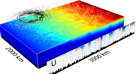
The numerical setup consists of a periodic channel configu-ration 2000 km long (Lx, zonal direction) and 3000 km wide (Ly, meridional direction) that aims to represent a zonal por-tion of the Southern Ocean located between 70 and 40◦S (Fig. 1). It is inspired by the experiment described in Aber-nathey et al. (2011), which is mainly adiabatic in the inte-rior. We add three ingredients to our reference experiment deemed essential to reach realistic levels of dissipation and whose consequence is to enhance dissipation and mixing in the model ocean interior.
2000 k
m
3000 k
m
4 k
m
Figure 1.Three-dimensional representation of instantaneous tem-perature (rectangular box, color scale ranges from 0 to 20◦C) and zonal velocity (vertical section) for the reference simulation at 2 km after 30 years. The domain is a 2000 km long and 3000 km wide reentrant channel. The configuration represents the Southern Ocean between 40 and 70◦S. Average ocean depth is 3500 m with irregular bottom topography, which limits the ACC (Antarctic Circumpolar Current) transport and tends to enhance deep mixing. At the surface, synoptic storms are included in the forcing. They generate NIWs, whose signature is visible in the velocity section, as a layering of the mesoscale structures.
breaking of internal lee waves (Nikurashin et al., 2011). Nevertheless, the deep flows impinging on bottom ir-regularities generate fine-scale shear, which enhances dissipation and mixing close to the bottom, as gener-ally observed in the Southern Ocean (Waterman et al., 2013).
ii. The surface and lateral forcing vary seasonally. The ob-jective is to reproduce a seasonally varying stratifica-tion and mixed-layer depth. These seasonal variastratifica-tions are known to be important in the formation process of mode waters and functioning of the overturning, since surface cooling triggers mixed-layer convection.
iii. The wind forcing includes idealized Southern Ocean storms. These high-frequency winds induce intense near-inertial energy and mixing into the ocean interior. From the analysis of scatterometer measurements, Pa-toux et al. (2009) provided general statistics of the spa-tial and temporal variability of the Southern Ocean mid-latitude cyclones for the period 1999–2006: most of the cyclones occurred between 50 and 70◦S, have a ra-dius between 400 and 800 km and last between 12 h and 5 days. Mesoscale cyclones lasting less than 4 days represent about 75 % of all cyclone tracks (Yuan et al., 2009). The storm forcing design, detailed in Ap-pendix A and adapting the methodology followed by Vincent et al. (2012), is based on these observations.
2.1 Configuration
The numerical code is the oceanic component of the Nucleus for European Modelling of the Ocean program (NEMO; Madec 2014). It solves the primitive equations discretized on a C-grid and fixed vertical levels (zcoordinate). Horizontal resolution of the reference simulation is 2 km. There are 50 levels in the vertical (with 10 levels in the upper 100 m and cells reaching a height of 175 m at the bottom), with a partial step representation of the topography. Sensitivity runs to both horizontal and vertical resolutions (1xbetween 1 and 20 km, 1x=2 km with 320 vertical levels) are an important part of this study. The model is run onβ-plane withf0=10−4s−1 at the center of the domain andβ=10−11m−1s−1. A third-order upstream biased scheme (UP3) is used for both tracer and momentum advection, with no explicit diffusion. The vertical diffusion coefficients are given by a generic length scale (GLS) scheme with ak−εturbulent closure (Reffray et al., 2015). Bottom friction is linear with a bottom drag coef-ficient of 1.5×10⁻³m s−1. We use a linear equation of state only dependent on temperature with linear thermal expan-sion coefficientα=2.10−4K−1. The temporal integration is achieved by a modified Leap Frog Asselin Filter (Leclair and Madec, 2009), with a coefficient of 0.1 and a time step of 150 s for the 2 km experiments. Sensitivity to these parame-ters and numerical choices are also performed.
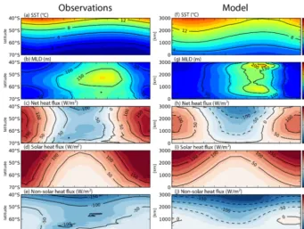
Air–sea heat fluxes are built so as to represent the ob-served seasonal evolution of the zonally averaged sea surface temperature and mixed-layer depth in the Southern Ocean (Fig. 2a, b). The surface heat fluxQnetis as follows:Qnet= Qsolar+Qnonsolar, whereQsolaris the shortwave heat flux and Qnonsolar the non-solar heat flux accounting for the effect of longwave, latent, sensible heat fluxes and a feedback termg (Tclim−Tmodel). This feedback term depends on a sensitivity termgset to 30 W m−2K−1(Barnier et al., 1995) and on the difference betweenTclim, a SST climatology that varies sea-sonally andTmodel the model SST. The seasonal amplitude ofQnetin the center of the domain is 200 W m−2(Fig. 2h), a value close to the observations (Fig. 2c). Over the northern 150 km of the domain, the temperature is relaxed toward an exponential temperature profile varying seasonally in the up-per 150 m. The response of the ocean to this forcing leads to a seasonal cycle of the surface temperature (Fig. 2f), and a deepening of the mixed layer from 30 m in summer to 150 m in winter (Fig. 2g), in good agreement with zonally averaged observations of the Southern Ocean (Fig. 2a, b). It is worth mentioning that the direct effect of a storm on the air–sea buoyancy flux (modulation of the radiative, latent and sensi-ble heat fluxes) is not explicitly accounted for.
The background mean wind stress that forces the experi-ments without storms is purely zonal:
τb=τ0sin
πy
Ly
Figure 2.Seasonal cycle of zonally averaged SST (a, f,◦C), mixed-layer depth (b, g, m) computed in both model and observations with a fixed threshold criterion of 0.2◦C relative to the temperature at 10 m, net air–sea heat flux (c, h, W m−2), and the solar (d, i, W m−2)and non-solar (e, j, W m−2)components of the air–sea heat flux. Climatological seasonal cycles are built from observations (left column) and model outputs and forcing. Observations include OAFlux products (Yu et al., 2007) for the period 1984–2007 and de Boyer Montégut (2004) mixed-layer depth climatology. Model data are from the last 10 years of the 2 km reference simulation without storms.
whereτ0=0.15 N m−2. In order to have exactly the same 10-year-mean wind stress between experiments with and with-out storms, the averaged residual wind due to the storm pas-sages is removed fromτbin the experiment with storms.
Two long reference experiments, one with storms and an-other without storms, with a horizontal resolution of 2 km have been run for 40 years. For these experiments, the model is started from a similar simulation without storms, equili-brated with a 200-year long spin-up at 5 km horizontal res-olution. Unless otherwise stated, the last 10 years of the simulations are used for diagnostics, excluding the northern 150 km band where restoring is applied. Similar long-term simulations with a horizontal resolution of 20 and 5 km have also been performed in order to determine meridional over-turning modifications with horizontal resolution (Sect. 7).
An experiment with a single storm traveling eastward through the center of the basin over an equilibrated ocean has also been performed. Initial conditions are taken from the 2 km horizontal resolution simulation (without storm) at (day) 31 December of year 30 from the 2 km reference exper-iment without storms. The storm is centered at the meridional positionLy/2 and has a maximum wind stress of 1.5 N m−2. The ocean spin-down response is analyzed for a period of 70 days (the storm is centered at days 5, starting at day 3 and ending at day 7).
In order to assess the sensitivity of interior mixing to numerics and storms characteristics, additional experiments have been run over shorter periods of 3 years, starting from year 30 of the 2 km reference experiment without storms. These experiments are summarized in Table 1 and will be analyzed in Sect. 5. The last 2 years of these experiments are used for diagnostics. Although the model is not equili-brated after a period of 3 years, we have verified in Sect. 5 that changes in terms of energy dissipation and mixing diag-nosed over this short period are significant.
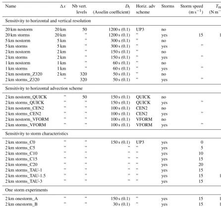
Table 1.Summary of numerical experiments.
Name 1x Nb vert. Dt Horiz. adv Storms Storm speed Tmax levels (Asselin coefficient) scheme (m s−1) (N m−2)
Sensitivity to horizontal and vertical resolution
20 km nostorm 20 km 50 1200 s (0.1) UP3 no
20 km storms 20 km ” 1200 s (0.1) ” yes 15 1.5 5 km nostorm 5 km ” 300 s (0.1) ” no
5 km storms 5 km ” 300 s (0.1) ” yes ” ”
2 km nostorm 2 km ” 150 s (0.1) ” no
2 km storms 2 km ” 150 s (0.1) ” yes ” ”
1 km nostorm 1 km ” 60 s (0.1) ” no
1 km storms 1 km ” 60 s (0.1) ” yes ” ”
2 km nostorm_Z320 2 km 320 50 s (0.1) ” no
2 km storms_Z320 ” 320 50 s (0.1) ” yes ” ”
Sensitivity to horizontal advection scheme
2 km nostorm_QUICK ” 50 150 s (0.1) QUICK no
2 km storms_QUICK ” ” 150 s (0.1) QUICK yes ” ” 2 km nostorm_CEN2 ” ” 100 s (0.1) CEN2 no
2 km storms_CEN2 ” ” 100 s (0.1) CEN2 yes ” ” 2 km nostorm_VFORM ” ” 100 s (0.1) VFORM no
2 km storms_VFORM ” ” 100 s (0.1) VFORM yes ” ”
Sensitivity to storm characteristics
2 km storms_C0 ” ” 150 s (0.1) UP3 yes 0 ”
2 km storms_C5 ” ” ” ” yes 5 ”
2 km storms_C10 ” ” ” ” yes 10 ”
2 km storms_C15 ” ” ” ” yes 15 ”
2 km storms_C20 ” ” ” ” yes 20 ”
2 km storms_TAU-1 ” ” ” ” yes 15 1
2 km storms_TAU-1.5 ” ” ” ” yes 15 1.5
2 km storms_TAU-3 ” ” ” ” yes 15 3
One storm experiments
2 km onestorm_A ” ” 150 s (0.1) ” yes 15 1.5 2 km onestorm_B ” ” 30 s (0.1) ” yes 15 1.5 2 km onestorm_C ” ” 150 s (0.01) ” yes 15 1.5
2.2 Energy diagnostics
Energy diagnostics and precise evaluations of the energy dis-sipation in the model are essential elements of our study. They are detailed below. The model kinetic energy (KE) equation can be written as follows:
1 2ρ0∂tu
2 h
| {z }
KE
=−ρ0uh(uh· ∇h) uh−ρ0uh·w∂zuh
| {z }
ADV
(1)
−uh· ∇hp
| {z }
PRES
+ρ0uh·Dh
| {z }
εh
+ρ0uh· ∇z(κv∇huh)
| {z }
εv
+Dtime,
where the subscript “h” denotes a horizontal vector,κvis the vertical viscosity,Dhthe contribution of lateral diffusion pro-cesses andDtimethe dissipation of kinetic energy by the time stepping scheme, which can be easily estimated in our sim-ulations since it only results from the application of the As-selin time filter. The dissipation of kinetic energy by spatial diffusive processes is computed as the spatial integral of the diffusive termsεvandεhin Eq. (1):
Ev= Z Z Z
ρ0uh· ∇z(κv∇zuh)
| {z }
εv
dxdydz (2)
=
Z Z Z
ρ0κv ∂uh
∂z · ∂uh
∂z
dxdydz
+ Z Z
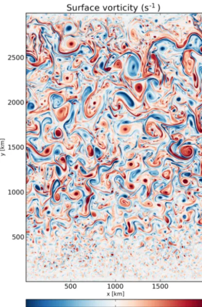
Figure 3. Surface vorticity snapshot (s−1)over the entire model domain at (day) 31 December of year 39 from the 2 km horizontal resolution experiment without storms.
Eh= Z Z Z
ρ0uh·Dh
| {z }
εv
dxdydz. (3)
As mentioned before, we do not specify explicit horizon-tal diffusion since it is implicitly treated by the UP3 advec-tion scheme we use (see numerical details in Madec, 2014). So the term Dh is evaluated at each time step as the dif-ference between horizontal advection momentum tendency computed with UP3 and the advection tendency given by a non-diffusive centered scheme alternative to UP3. Two op-tions are the second-order and fourth-order schemes imple-mented in NEMO. The second-order scheme is non-diffusive but dispersive. The fourth-order scheme in NEMO involves a fourth-order interpolation for the evaluation of advective fluxes but their divergence is kept at second order, making the scheme not strictly non-diffusive. Although the estima-tion of UP3 horizontal diffusion depends on the scheme used as a reference, we verify in Sect. 5 that the sensitivity of domain-averaged εh to the choice of the second- or fourth-order scheme is much smaller than that resulting from other parameter changes, e.g., small changes in the characteristics of the atmospheric forcing.
3 Ocean dynamics under low-frequency forcing
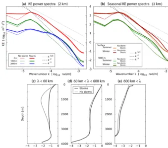
We first examine the dynamics and mean state of the experi-ment with a horizontal resolution of 2 km and without storms in order to review the background oceanic conditions within our zonal jet configuration. A snapshot of the surface vortic-ity field (Fig. 3) illustrates the broad range of scale resolved by the 2 km model and the ubiquitous presence of meso- and submesoscale motions, including eddies and filaments. The slope of the annual mean surface velocity spectrum in the meso- and submesoscale range is betweenk−2andk−3. The spectral slope varies seasonally (Fig. 4b), more noticeably in the submesoscale range (60 km >λ; i.e., horizontal scales below 10 km), betweenk−3during summer andk−2during winter (for the meso- and submesoscale range in Fig. 4b, the thin dark red line is superimposed on the thick dark red line). We interpret the increase of submesoscale energy dur-ing winter as a direct consequence of enhanced mixed-layer instabilities in response to a deep mixed layer (Fox-Kemper, 2008; Sasaki et al., 2014).
The energy contained at large scale and mesoscale (k < 5×10⁻⁵rad m−1)decreases with depth as indicated by the spectra at 1000 and 2500 m (Fig. 4a). But note that the en-ergy contained in the wavenumber range 5×10⁻⁵< k <6×
10−4rad m−1(i.e., the range associated with small mesoscale bordering with the submesoscale) is larger at 2500 m com-pared to 1000 m. This is due to an injection of energy at these scales by the rough topography. As shown by instanta-neous velocity sections in Fig. 5a and b, the horizontal scales ofuandvbelow 2500 m are much shorter than the typical scale of the upper-ocean mesoscale field. They correspond to the scale of the bathymetry, and are responsible for in-creased horizontal shear in the deep ocean (Fig. 5e), thereby contributing to the dissipation of the energy imparted by the winds to the mean flow.
Vertical velocity rms is below 10 m day−1over most of the water column except near the bottom (i.e., below 2500 m) where it increases substantially to∼100 m day−1(Figs. 5c and 6b). Although flat bottom numerical solutions can also exhibit similar increases (Danioux et al., 2008), the spa-tiotemporal scales ofw near the bottom (e.g., see Fig. 5c) suggest the importance of flow–topography interactions.
The average zonal transport in the reference experiment is
sur-Figure 4.Horizontal velocity variance in the 2 km reference experiments with and without storms.(a)Kinetic energy power spectra as a function of wavenumber (rad m−1)at 0, 1000 and 2500 m depth.(b)Seasonal (summer is defined as December–January–February and winter as June–July–August) kinetic energy power spectra at 0 and 1000 m depth. Spectra are built using instantaneous velocity taken each 5 days of the last 2 years of the 2 km simulations. Kinetic energy contained in the wavelength rangesλ <60 km(c), 60 km< λ <600 km(d) andλ >600 km(e)as a function of depth. In(b)and for wavenumber above 5×10⁻⁵rad m−1, the winter surface spectra with and without storms (dark red thin and thick lines) are superimposed, as well as the summer and winter 1000 m spectra without storms (light and dark green thin lines).
face (Fig. 6a). Such a level of energy is typical of ocean storm tracks of the Southern Ocean (e.g., Morrow et al., 2010).
The clockwise cell of the Eulerian overturning streamfunc-tion ψ (Fig. 7a)1 illustrates the large-scale response to the northward Ekman transport (that acts to overturn the isopyc-nal) and the irregular return flow in the deep layers due to bottom topography. This transport is largely compensated by an eddy-induced-opposing transport, leading to a resid-ual circulation (see e.g., Marshall and Radko, 2003). This residual MOC can be computed as the streamfunctionψiso from the time- and zonal-mean transport in isopycnal coor-dinates (e.g., Abernathey et al., 2011). In the lightest den-sity classes and northern part of the domain, the counter-clockwise cell (negative, driven by surface heat loss) is the signature of a poleward surface flow and equatorward re-turn interior flow, which can be interpreted in terms of mode 1Throughout the paper, Eulerian and residual meridional trans-ports obtained from our 2000 km long channel are multiplied by 10 in order to make them directly comparable to those for the full Southern Ocean, whose circumference is∼20 000 km.
Figure 5.Model snapshots of a 2 km simulation at a mesoscale eddy location 2 days before (top) and 17 days after (bottom) the passage of a storm:(a, f)zonal velocity (m s−1),(b, g)meridional velocity (m s−1),(c, h)vertical velocity (m s−1),(d, i)vertical shear (s−2)and (e, j)horizontal strain (s−2). Snapshots after the passage of the storm(e–h)are taken 50 km eastward in order to account for the advection of the core of an anticyclonic mesoscale eddy. Isotherm are shown in the left panels ((a),(b),(f)and(g)) with contour intervals of 1.25◦C from 2.5 to 10◦C. Before the passage of the storm the simulation has been equilibrated without high-frequency forcing, so the solution at day 2 is free of wind-forced NIWs. The snapshots shown here correspond to day 2 and 22 in the time axis of Fig. 8. We choose day 22 to leave enough time for the NIWs to reach the base of the anticyclonic eddy.
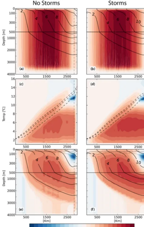
Figure 7. Eulerian mean streamfunctionψ (a, b), MOC stream-function diagnosed in isopycnal coordinates (c ,d)and projected back to depth coordinates(e, f)from 10-year long 2 km equilibrated simulations with (right) and without storms (left). Units are Sv and the contour interval is 0.25 Sv. Temperature contours corresponding to 2, 4, 6, 8, 10, 12 and 14◦C are indicated in(c, d). Positive cells are clockwise. The dashed lines in(c, d)represent the 10, 50 and 90 % isolines of the cumulative probability density function for sur-face temperature (following Abernathey et al., 2011), which indi-cate how likely a particular water mass is to be found at the surface exposed to diabatic transformation. Dotted lines in(e, f)represent (from top to bottom) the 90, 50 and 10 % isolines of the cumula-tive probability density function for mixed-layer depth. The verti-cal dashed line aty=2850 km represents the limit of the northern boundary damping area. Model transports have been multiplied by 10 in order to scale them to the full Southern Ocean.
it is of no concern for our purpose. In the 2 km reference case without storms, the transport by the main clockwise cell of the MOC streamfunction results in a realistic overturning rescaled value of 18 Sv (Table 2).
Table 2. Maximum of the clockwise cell (as in the context of Fig. 7) of the overturning streamfunctionψiso (Sv) averaged be-tweeny=2000 km and y=2500 km. The streamfunctions have been computed using 10 years of 5-day average outputs from equi-librated experiments. Model transports have been multiplied by 10 in order to scale them to the full Southern Ocean.
20 km 5 km 2 km
No storm 20.4 Sv 19.4 Sv 18.0 Sv Storms 20.7 Sv 20.9 Sv 21.0 Sv
4 Single-storm effect
As a first step, it is useful to consider a situation in which a single storm disrupts the quasi-equilibrated flow described in the previous section so that high-frequency forcing effects can be more easily identified. The storm is chosen to travel eastward through the center of the domain. The experiment is thoroughly described in Sect. 2 and the ocean spin-down response is analyzed in Figs. 5, 8, 9 and 10 for a period of 70 days (the storm starts at day 3 and ends at day 7). 4.1 NIW generation and propagation
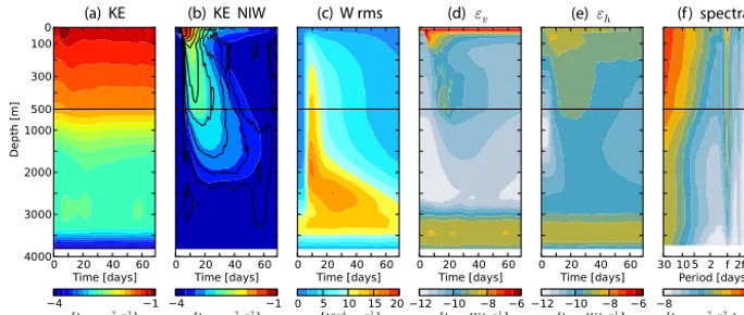
After the passage of the storm, the horizontal currents be-tween the surface and 1500 m exhibit a layered structure with typical vertical scales of ∼100–200 m (Fig. 5f, g), which contrasts with the homogeneity of the mesoscale currents be-fore the passage of the storm (Fig. 5a, b). The layering is sim-ilar to that observed in a section across a Gulf Stream warm core ring by Joyce et al. (2013). It is associated with an in-crease of the horizontal and vertical shear in the ocean inte-rior (Fig. 5i, j). In agreement with Danioux et al. (2011), we encounter that the storm intensifies the vertical velocities in the whole water column (Fig. 5h). In response to the storm, KE in the upper 100 m is strongly increased during 5 days (Fig. 8a). An intensification of KE is also observed in the fol-lowing days at depths below 500 m, indicative of downward propagation of the energy. A large part of the additional en-ergy injected by the storm occurs in the near-inertial range (Fig. 8b): the space–time distribution of the near-inertial en-ergy (colors) matches rather well the difference of KE be-tween the experiment with a storm and a control experiment without a storm starting from exactly the same initial condi-tions (contours).
(b) KE NIW (c) W rms
(a) KE (d) (e) (f) spectra
day
Figure 8.Response of the ocean to the passage of a single storm:(a)horizontal kinetic energy (log10m2s−2),(b)horizontal kinetic energy in the NIW band (colors, log10m2s−2)and difference of horizontal kinetic energy between the simulation with storms and a reference simulation without storms (iso-contours),(c)rms of the vertical velocity (10−4m s−1)defined as
q
w2, whereτθ=τmaxRr is the horizontal average operator,(d)εvenergy dissipation due to vertical diffusion (W kg−1)and(e)εhthe energy dissipation due to horizontal diffusion (W kg−1). These diagnostics are spatially averaged betweenLy/3 and 2Ly/3. The spatially averaged power spectra of the meridional velocity (log10m2s−2day−1)is shown in(f)and has been computed using hourly data from day 0 to day 70. The storm starts at day 3 and ends at day 7.
range estimated by Cuypers et al. (2013) for NIW packets forced by tropical storms in the Indian Ocean. Vertical veloc-ities are generally intensified in the depth range where strat-ification is weakest but the maximum of rms vertical veloc-ities qualitatively follows a similar behavior as near-inertial KE: it peaks at 2000 m depth a few days after the storm ini-tiation, and then propagates downward the following weeks (Fig. 8c).
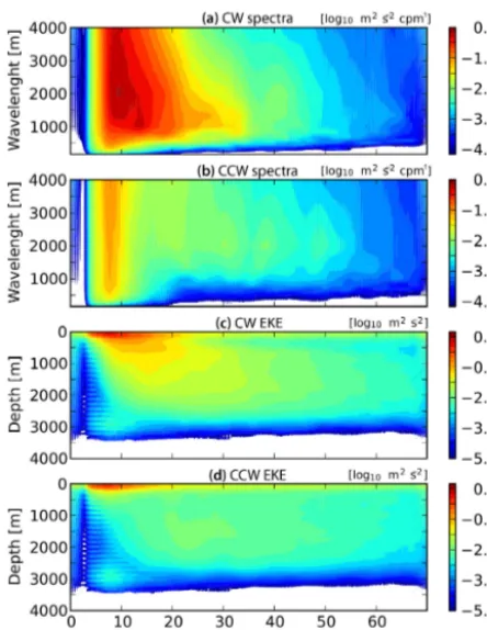
Rotatory polarization of the near-inertial waves is use-ful to separate the upward- and downward-propagating con-stituents of the waves. Rotatory spectra (details of the methodology are given in Appendix B) of the stretched pro-files of velocity allow for a separation of the clockwise (CW) and counter-clockwise (CCW) contributions to the energy as a function of time and vertical wavenumber (Fig. 9a, b). Most of the energy is contained in the CW part of the spec-tra, i.e., most of the energy propagates downward. While the energy directed downward and contained in wavelengths be-tween 1000 and 2000 m remains strong for about 30 days, the energy at short wavelengths (< 500 m) is rapidly dissipated both for downward- and upward-propagating NIWs. The near-inertial KE computed from Wentzel–Kramers–Brillouin (WKB)-stretched CW and CCW velocities (see Appendix B for details) are shown in Fig. 9c and d. Between days 20 and 30, the KE of CCW waves exhibits a maximum cen-tered around 1500–2000 m. Because the highest topographic features only reach up to 3000 m depth; furthermore, since near-inertial velocities have been WKB scaled, we interpret this local maximum as the signature of interior reflection. During the 5 days following the passage of the storm, we notice a slight increase of both CW and CCW KE below 2500 m depth, suggesting NIW generation at the bottom in
response to storm forcing. Associated energy levels are lim-ited (< 10−2m2s−2)and no sign of vertical propagation is observed so this process must be of minor importance, com-pared to other flow–topographic interactions acting in the same depth range such as lee-wave generation by the bal-anced circulation (Nikurashin and Ferrari, 2010).
Horizontal velocity frequency spectra computed at each depth and averaged over the entire 70-day period of the ex-periment are shown in Fig. 8f. They exhibit energy peaks at f, 2f and to a lesser extent 3f. The near-inertial and super-inertial peaks are surface intensified but have a signa-ture throughout the water column. Waves with super-inertial frequency arise after a few inertial oscillations and are exited by non-linear wave–wave interactions (Danioux et al., 2008). 4.2 Dissipation of the NI energy
Figure 9. Temporal evolution of clockwise (CW) and counter-clockwise (CCW) spectra as a function of vertical wavelength, com-puted from Wentzel–Kramers–Brillouin (WKB)-stretched near-inertial velocities(a, b)for the single-storm experiment. Units are m2s−2cpm−1. Near-inertial KE computed as a function of time and depth from CW- and CCW-stretched velocities are shown in(c) and(d). Units are m2s−2.
is due to a slight strengthening of the large-scale eastward surface current in response to the storm (not shown). This strengthening is a consequence of the zonal current distribu-tion as a funcdistribu-tion of latitude, which is not symmetric with re-spect toy=1500 km, so the domain average additional zonal wind work imparted by the storm is nonzero and positive. At day 70, 61.4 % of the kinetic energy has been dissipated by diffusive processes in the upper 200 m, while 11.1 % has been dissipated between 200 and 2000 m and 4.3 % between 2000 m and the bottom (see Table 3). Bottom friction (5.9 %) and pressure gradients (5.5 %) are also limited sinks for the energy imparted by the storm. The cumulated contributions of horizontal advection and Coriolis forces are small com-pared to the other terms (< 1 %). The contribution of the Cori-olis force to the energy budget is not precisely zero due to the staggered location ofuandvpoints in our Arakawa C-grid. Most of the dissipation due to viscous processes is achieved by vertical processes in the upper 200 m (80 %, Fig. 10c). The maximum contribution of horizontal dissipation is be-tween 200 and 2000 m where it is stronger than vertical dis-sipation (Fig. 10c).
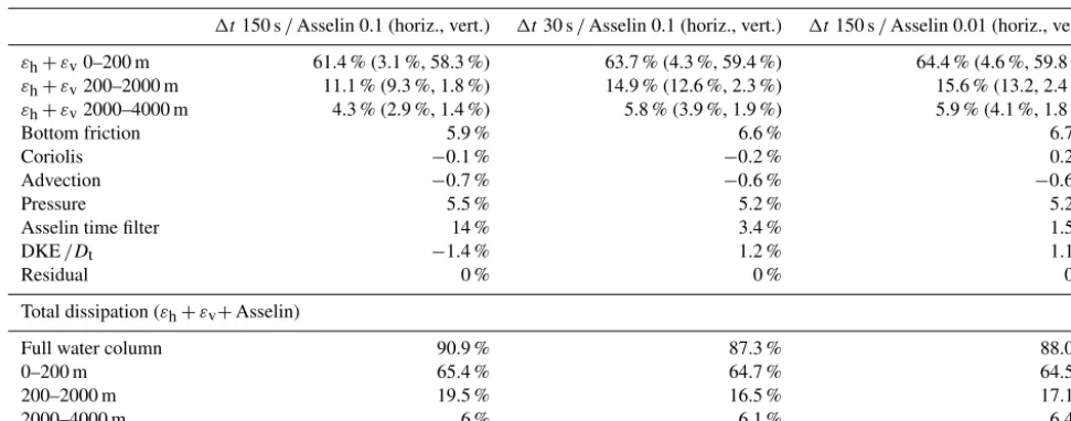
Table 3.Cumulated energy dissipation at day 70 (see Fig. 10) relative to a reference experiment without a storm, for three single-storm experiments with different time step and Asselin time filter coefficient. Results for the reference experiment described in Figs. 5, 8–10 are shown in the first column.
1t150 s/Asselin 0.1 (horiz., vert.) 1t30 s/Asselin 0.1 (horiz., vert.) 1t150 s/Asselin 0.01 (horiz., vert.)
εh+εv0–200 m 61.4 % (3.1 %, 58.3 %) 63.7 % (4.3 %, 59.4 %) 64.4 % (4.6 %, 59.8 %)
εh+εv200–2000 m 11.1 % (9.3 %, 1.8 %) 14.9 % (12.6 %, 2.3 %) 15.6 % (13.2, 2.4 %)
εh+εv2000–4000 m 4.3 % (2.9 %, 1.4 %) 5.8 % (3.9 %, 1.9 %) 5.9 % (4.1 %, 1.8 %)
Bottom friction 5.9 % 6.6 % 6.7 %
Coriolis −0.1 % −0.2 % 0.2 %
Advection −0.7 % −0.6 % −0.6 %
Pressure 5.5 % 5.2 % 5.2 %
Asselin time filter 14 % 3.4 % 1.5 %
DKE/Dt −1.4 % 1.2 % 1.1 %
Residual 0 % 0 % 0 %
Total dissipation (εh+εv+Asselin)
Full water column 90.9 % 87.3 % 88.0 %
0–200 m 65.4 % 64.7 % 64.5 %
200–2000 m 19.5 % 16.5 % 17.1 %
2000–4000 m 6 % 6.1 % 6.4 %
Further insights on the distribution of viscous dissipation are obtained by examining the temporal evolution ofεvand εhat all depths (Fig. 8d, e). It shows that the largest kinetic energy dissipation rates are achieved byεvin the upper 100 m during the 10 days following the storm (Fig. 8d). Interest-ingly we note the presence of a maximum ofεvbetween 300 and 500 m depth between days 10 and 40, with value of order 10−9W kg−1. This is due to large shear/dissipation values at depth in and below the core of anticyclonic structures as il-lustrated in Fig. 5 and confirmed in Sect. 5. At these inter-mediate depths,εhandεhare of comparable magnitude. No significant near-bottom increase ofεv orεhis found during or after the storm passage in Fig. 8d and e, although NIWs are generated at the bottom in response to the passage of the storm (as seen in the previous section, Fig. 9d). The levels of near-inertial energy below 2500 m depth remain 2 to 3 orders of magnitude lower than those found in the mixed-layer and are not sufficient to significantly increase bottom dissipation. The time filter contributes to dissipate 14 % of the energy imparted by the storm, with dissipation well distributed in the entire water column (Fig. 10d). This dissipation is highly dependent of the time step used in the simulation (150 s) and “Asselin time filter” coefficient (0.1, the default value used in most of the studies with NEMO). In a similar experiment with a time step of 30 s, the contribution of the Asselin time filter falls to 3.4 % (see Table 3) and with an Asselin coef-ficient of 0.01 it falls to 1.5 %. This is coherent with tem-poral diffusion of the Asselin time filter being proportional to the product of the Asselin coefficient by the model time step (Soufflet et al., 2016). The temporal diffusion is divided by 5 when using a time step of 30 s instead of 150 s, and the temporal diffusion is divided by 10 when using a coef-ficient equal to 0.01 instead of 0.1. In these two sensitivity
experiments, the energy that is not dissipated by the tempo-ral filter is dissipated by latetempo-ral and vertical diffusion in the entire water column, leading to a vertical distribution of to-tal dissipation (Asselin+εh+εv), which is similar between experiments (see Table 3).
In terms of meridional distribution, most of the energy is dissipated below the storm track (Fig. 10e). This ques-tions the common hypothesis that a significant part of the energy could be radiated away from the generation area to-ward lower latitudes (e.g., Garrett, 2001; Zhai et al., 2004; Blaker et al., 2012; Komori et al., 2008). In our configuration it appears that vertical propagation and dissipation act much faster than horizontal propagation.
5 Storm effects in quasi-equilibrium
Table 4.Two-year mean KE balance (mW m−2)averaged over the entire domain for the 2 km reference experiments with (left) and without storm (right). The percentages give the fraction of total wind work that is balanced by the terms of the KE equation. The second series of numbers and percentages in the storm column refers to the storm−no storm differences.
2 km [mW m−2] 2 km+STORMS [mW m−2] Differences [mW m−2]
DKE/Dt −0.1 0.02
Wind work 12.43 16.08 +3.65
Vertical dissipation −2.90 (23.4 %) −5.32 (33.1 %) −2.42 (66.3 %) Horizontal dissipation −0.65 (5.2 %) −1.09 (6.8 %) −0.44 (12.0 %) Pressure work −4 (32.2 %) −4.18 (26.0 %) −0.18 (5 %) Bottom friction −4.84 (38.9 %) −4.91 (30.5) −0.07 (2 %) Advection −0.03 (0.2 %) 0.01 (0.1 %) −0.02 (0.5 %) Coriolis −0.08 (0.6 %) −0.06 (0.4 %) −0.02 (0.5 %) Asselin time filter −0.01 (0.1 %) −0.45 (2.8 %) −0.44 (12 %)
Residual 0 0 0
of KE dissipation and the sensitivity of this dissipation to nu-merics.
5.1 EKE in the 2 km reference experiments
The additional input of energy by the storms modifies the levels of kinetic energy in the flow. In the 2 km case with-out storms, the domain-averaged 10-year mean KE computed from zonally averaged velocities is 1.14×10⁻³m2s−2and the EKE (i.e., 1/2(u02+v02)where primed velocity anoma-lies are defined with respect to zonally averaged velocities) is 5.21×10⁻³m2s−2. When storms are included, both quan-tities increase (mean KE increases to 1.21×10⁻³m2s−2and mean EKE increases to 5.34×10⁻³m2s−2). Besides this overall EKE increase, EKE is decreased in the upper 300 m (Fig. 6a). Our interpretation is that this arises owing to the storm reduction of the stratification (Fig. 6d). In turn, this impacts the structure of the vertical modes and the inverse energy cascade in a way that favors a less surface intensified distribution of EKE with storms (Smith and Vallis, 2002). The small enhancement of EKE in the range 1000–2000 m in the storm simulation is consistent with this interpretation. There are other impacts of the storms: the rms of the vertical velocity is increased by 1 order of magnitude in the whole water column and reaches values on the order of 10−3m s−1 (Fig. 6b); the upper 100 m of the ocean get warmer and less stratified (Fig. 6c, d); and the mixed-layer deepens by∼30 m (horizontal lines in Fig. 6c). Obviously, the heat budget is also affected with a+5 W m−2increase of the downward tur-bulent heat fluxes (Fig. 6e) and air–sea heat fluxes (vertical lines in Fig. 6e).
The ability of near-inertial oscillations to propagate into the ocean interior is affected by the mesoscale field (through the chimney effect, as it will shown in Sect. 5.3) but is also in-timately tied to the shrinking of their horizontal scales so we expect to see non-trivial modifications of the KE wavenum-ber spectra in the presence of storms. Near the surface the storms impact is mainly perceptible at the lowest
wavenum-bers, the storms forcing scale (Fig. 4a, e) or during summer at the submesoscale (Fig. 4b). This larger influence of the storms during summer compared to winter in the subme-soscale range is explained by a larger impact of the storms on the mixed-layer depth in summer compared to winter (not shown). During summer, the mixed-layer is shallow (Fig. 2b, g) and sensitive to direct mixing by the storms while during winter the mixed-layer is deeper and its depth is con-trolled at first order by convective processes with storm pas-sages having a weaker influence. Modifications of the spec-tral slope (∼2.5) by the storms are almost insignificant in the meso-/submesoscale range, where surface dynamics en-ergizes the flow, particularly at scales∼10 km (wavelength
∼60 km) and below (Fig. 4a, d). The effect of storms at such fine scales becomes pronounced below∼300 m (Fig. 4c), where the surface mode becomes attenuated2.
At 1000 m where the fine-scale energy associated with the NIW is largest (Fig. 4c), the energy spectrum presents a bulge in the wavenumber range 10−4< k <10−3rad m−1that at-tests of the energy input at such scales. This energy input is larger during winter than during summer (Fig. 4b) in agree-ment with the storm forcing, which is more energetic dur-ing winter. Fine-scales energization by the NIW can be seen down to ∼2500 m (Fig. 4c) where it is confined to lower wavelength than at 1000 m (k >3×10⁻⁴rad m−1). Limited signs of a large-scale energy enhancement by the storms can be found at 1000 and 2500 m.
5.2 KE budget and dissipation in the 2 km reference experiments
Let us first examine in detail the KE balance (Table 4) in the two 2 km reference experiments with and without storms. The KE balance in both experiments are very similar, with 2The typical vertical scale H (k) of the surface mode at a
wavenumberkisH (k)∼f/(N k). UsingN=
r
2×10⁻⁵
(see
Figure 11.Kinetic energy dissipation (ε; W kg−1)as a function of depth in experiments at 2 km with storms (continuous lines) and without storms (dashed lines): total energy dissipationεwith and without storms(a), dissipation due to vertical processesεvand dissipation due to horizontal processesεh(b),εhcomputed from a second-order (UBS-C2) or fourth-order (UBS-C4) centered scheme (see text for details) together with a 20-year mean and standard deviation ofεfor the 2 km reference experiment(c), and summer (December–January–February) and winter (June–July–August)ε. Profiles are computed using 5-day snapshots of the entire domain for a 2-year period. Position, strength and duration of the storms remain strictly equal in the different experiments.
overall wind work mainly balanced by the work done by bot-tom friction (38.9 % without storms and 30.5 % with storms), pressure work maintaining the system available potential en-ergy (32.2, 26.0 %) and vertical diffusion (23.4, 33.1 %). The KE balance also indicates that the additional input of en-ergy provided by the storms (+3.64 mW m−2)is balanced at 90 % by dissipation (−2.86 mW m−2 for horizontal and vertical dissipation to which one should add the Asselin filter contribution) with pressure work and bottom friction being secondary (−0.18 mW m−2 representing a 5 % contribution and−0.07 mW m−2representing a 2 % contribution). This is in stark contrast with the equilibration of the low-frequency wind work feeding the balanced circulation.
Now let us focus on the spatial and seasonal distribution of the horizontal and vertical KE dissipation termsεhandεv. The vertical distribution of these terms are computed using instantaneous outputs available every 5 days during the last 2-year of the 2 km runs. This choice of a limited 2-year pe-riod is justified given the smallness of the standard deviation of annual meanεcomputed using 20 years of simulation of the experiment with storms (Fig. 11c), e.g., compared to ε differences we present for different experiments. As stated in Sect. 2, we estimate UP3 intrinsic horizontal diffusivity as the difference between UP3 momentum tendency and the tendency given by a fourth-order advective scheme. The
al-ternative use of a second-order advection scheme produces very similar estimates ofεh(Fig. 11c).
Overall energy dissipation (ε=εh+εv)in the reference experiments is increased by 1 order of magnitude or more over most of the water column in the presence of storms (Fig. 11a). Exception is found in the lowest 1000 m, where dissipation is always strong because of the interaction of the mesoscale and large-scale field with the topography. Without storms, dissipation reaches a minimum of 3×10⁻¹²W kg−1 between 1000 and 1500 m depth while the presence of storms increases the level of dissipation to > 10−10W kg−1 in this depth range, in agreement with the results for the single-storm experiment (Fig. 8).
Figure 12.εhandεv(W kg−1)distribution within composite cyclones (top) and anticyclones (bottom) identified in the 2 km experiments without storms (left) and with storms (right). The black iso-contours are isotherms from 2 to 8◦C andσ/f iso-contours are shown in white (0.9, 0.95 and 0.98σ/f ), withσ=f+ξ /2 the effective frequency andζ the relative vorticity. Composites are built using 10 years of 5-day-averaged model outputs, betweenLy/3 and 2Ly/3. A total of 8167 cyclone and 8878 anticyclone snapshots have been identified in the experiment without storms and 7306 cyclone and 8037 anticyclone snapshots in the experiment with storms.
Since the air–sea heat fluxes and the strength of the storms follow a seasonal cycle, we expect some seasonality of both near-surface and interior dissipation. This is examined by comparing εprofile in summer and winter (Fig. 11d). Val-ues of ε in the upper 300 m display large differences be-tween summer and winter, in both experiments with or with-out storms. Increased upper-ocean energy dissipation during winter is explained by mixed-layer convection in response to surface heat loss. Below 300m, the experiment with storms is the only one that displays seasonal variations of ε, with greatest values during winter. This is consistent with obser-vations by Wu et al. (2011), who observed a seasonal cycle of diapycnal diffusivity (hence ofε) in the Southern Ocean at depths down to 1800 m, although it reaches somewhat deeper (∼2500 m) in our solutions.
5.3 How do mesoscale eddies shape KE dissipation?
Mesoscale activity is known to affect NIW penetration into the ocean interior (Danioux et al., 2011). In order to clarify the role of mesoscale structures on energy dissipation distri-bution, an eddy detection method is used to produce com-posite averages of dissipation, relative to eddy centers. The identification of the eddies is based on a wavelet decomposi-tion of the surface vorticity field (e.g., Doglioli et al., 2007). Following Kurian et al. (2011) a shape test with an error
cri-terion of 60 % is used to discard structures with shapes too different from circular. Since the Rossby radius of deforma-tion varies meridionally within the model domain, compos-ites are built with eddies located betweenLy/3 and 2Ly/3, and with an area larger than 400 km2. The barycenter is taken as the center of the eddies and used as reference point to build the composites.
The general distribution ofεhandεvwithin composite ed-dies (Fig. 12) is in agreement with the vertical distribution of domain-averagedεdiscussed in the previous section, with increased values ofεhandεvnear the surface and the bottom. But the composites also highlight the impact of eddies on the distribution ofεhandεv. As discussed below the distribution of the kinetic energy dissipation within eddies is very differ-ent depending on the presence or absence of storms.
Figure 13.Kinetic energy dissipation (ε; W kg−1)as a function of depth in experiments at 20, 5, 2 and 1 km horizontal resolution, with storms (continuous lines) and without storms (dashed lines): total energy dissipationεwith storms(a)and without storms(b), dissipation due to vertical processesεvwith storms(c)and without storms(d), dissipation due to horizontal processesεhwith storms(e)and without storms(f), and the fraction of the total dissipation due to vertical processes (εv/εin %) (gandh). As in Fig. 11, profiles are computed using 5-day snapshots of the entire domain for a 2-year period. Position, strength and duration of the storms remain strictly equal in the different experiments. The experiment z320 has an horizontal resolution of 2 km but 320 vertical levels, ranging from 1 m at the surface to 250 m at the bottom (below 2500 m depth the vertical size of the cells is the same as in the 2 km reference experiment).
In the presence of storms (Fig. 12e–h), εv andεh peak at the base of the anticyclones with values higher than 10−9W kg−1, in qualitative agreement with various observa-tions of NIW trapping at the base of the anticyclones (Joyce et al., 2013; Kunze et al., 1995). The largest dissipation is bounded by the contourσ=0.95f withσ=f+ξ /2 the ef-fective frequency. The compositing highlights the dispropor-tionate importance of anticyclones for NIW dissipation. The total area occupied by the anticyclones that have been picked up by the eddy detection method represents only 2.6 % each
Figure 14.Kinetic energy dissipation (ε) and wind work as a function of model resolution, in experiments with (continuous lines) and without storms (dashed lines):(a)wind work and energy dissipation integrated from surface to bottom (mW m−2),(d)energy dissipation integrated from surface to bottom (decomposed into contributions fromε, bottom friction and Asselin time filter; mW m−2)and total dissipationε (W kg−1)averaged in the depth ranges 0–100 m(b), 100–400 m(c), 400–1000 m(d)and 1000–2000 m(e). Values are computed using 5-day snapshots of the entire domain for a 2-year period as in Fig. 9. Isolated dots representεfor the 2 km experiment with 320 vertical levels. Wind work(a)and energy dissipation contributions(d)have only been computed for the 20, 5 and 2 km experiments.
5.4 Sensitivity tests
How dissipation changes when key physical and numerical parameters are varied is examined below.
Horizontal resolution. Energy dissipation is compared in experiments at 20, 5, 2 and 1 km horizontal resolution (Fig. 13). The sensitivity to resolution strongly depends on the considered depth range. Near the surface (0– 100 m) the dissipation is almost not sensitive to the res-olution (Figs. 13a, b and 14b). This is coherent with the relatively weak variations of the wind work from one resolution to another (Fig. 14a). But below (100– 400 m), experiments with or without storms show a de-crease of ε when increasing resolution (Figs. 13a, b and 14c). This decrease is not related to modifications of the wind work (Fig. 14a) and occurs in a depth range affected by upper-ocean convection. So it may mostly result from the weakening of the dissipation due to upper-ocean convection when resolution increases, as highlighted by the shallowing of the mixed-layer depth (with storms and (without storms): 101 m (93m) at 1x=20 km, 87 m (67m) at1x=5 km, 80 m (59m) at 1x=2 km and 68 m (53m) at1x=1 km). This would be in agreement with the re-stratifying effect of the mesoscale and sub-mesoscale flow, which become more efficient when resolution increases (e.g., Fox-Kemper, 2008; Marchesiello et al., 2011).
In the depth range 400–3000 m, the sensitivity to reso-lution is highly dependent on the presence or absence of storms. Without storms, a major reduction of dissipation with increasing resolution is noticeable (Fig. 13b). This
reduction is of a factor 10 or more in the depth range 400–2000 m, when going from 20 to 1 km resolution (Figs. 13b and 14c, e, f). Concomitantly, the fraction of dissipation due to vertical shear increases because that corresponding to lateral shear drops most rapidly (Fig. 13h). At 1km resolution, it is systematically above 20 % down to ∼2000 m and reaches 50 % at 1500 m depth. This contrasts with the run at 20 km where εv is never more than 7 % of the total dissipation over the same depth range.
relate this maximum to the one seen in dissipation com-posites for anticyclones (Fig. 12).
Near the bottom important changes also take place when increasing resolution: vertical (horizontal) dissipation decreases (increases), which leads to a slight decrease in dissipation by interior viscous processes. Instead, dis-sipation by bottom friction increases significantly with resolution (Fig. 14d). We are not sure how to inter-pret these bottom sensitivities, especially since we do not properly resolve the processes implicated in flow– topography interactions (Nikurashin and Legg, 2011). Vertical resolution. An experiment with 320 vertical
lev-els has been carried out in which vertical shears (and high-order vertical modes) are better represented than with the reference 50 levels. The vertical thickness of the cells increases from 2 m at the surface, 5 m at 500 m depth, 70 m at 1000 m depth and 180 m near the bot-tom. The size of the cells below 2500 m are equal to the reference experiment so that the local characteristics of flow–topography interactions are unchanged. The over-all dissipationεis increased in the presence of storms in the interior in the configuration with 320 vertical levels (Figs. 13a, b and 14c–e), indicating that the downward propagation of the NIE is better resolved in the high vertical resolution experiment with more NIE available at depth. A similar increase ofεin the upper 100 m in the experiments with and without storms (Fig. 14b) sug-gests that mixed-layer dynamics is profoundly altered when changing the vertical resolution.
Advection schemes. The reference experiment relies on an UP3 advection scheme (Webb et al., 1998). It is com-pared with three experiments run with three widely used advection scheme: the QUICK (Quadratic Upstream In-terpolation for Convective Kinematics) scheme, which is the default scheme of The regional oceanic modeling system (ROMS) model (Shchepetkin and McWilliams, 2005) and also includes implicit diffusion; a second-order centered scheme with a horizontal biharmonic viscosity of−109m4s−2; and a second-order centered scheme with the vector invariant form of the momen-tum equations (Madec, 2014) with the same horizontal biharmonic viscosity. The implicit dissipation of UP3 and QUICK take the form of a biharmonic operator with an eddy coefficient proportional to the velocity (Ah= −|u|1x3/12 with UP3 and Ah= −|u|1x3/16 with QUICK). Although QUICK is by construction less dissipative compared to UP3,εin both experiments are very similar (Fig. 15a). With or without storms, the second-order scheme in flux form (CEN2) or vector in-variant form (VFORM) leads to increasedεin the ocean interior with the increase being the largest at the bottom (the energy dissipation profiles for the second-order and the vector-form scheme are so close that they are
su-perimposed in Fig. 15a). Such distribution of the dis-sipation changes is obviously related to the choice of a biharmonic coefficient of −109m4s−2: characteris-tic velocities of 1.5 and 2 m s−1 are required for UP3 and QUICK schemes to match a biharmonic diffusion coefficient of−109m4s−2. So near the surface where currents are strong the explicit diffusion in the simula-tions with second-order schemes is of same order as the implicit diffusion in QUICK/UP3 simulations, while at depth an explicit biharmonic operator with coefficient
−109m4s−2 overestimates the diffusion compared to UP3/QUICK implicit diffusion. We also note a dissi-pation increase in the depth range 1000–2000 m when using these schemes in the presence of storms. Sensitiv-ity closer to the surface is much more limited.
Maximum wind speed. Stronger winds increase the energy dissipation in the interior (Fig. 15c). Changes in dissi-pation levels take place from the near surface down to 2500–3000 m, which again highlights that near-inertial energy is able to propagate down to such depths. Dis-sipation changes induced by modifications of the flow– topography interactions would also yield changes in dis-sipation near the bottom, which is not the case, particu-larly when comparing the 1 and 1.5 N m−2experiments. Storm speed. The storm speed of the reference experi-ment was taken asCs=15 m s−1, a value close to the 12 m s−1inferred by Berbery and Vera (1996) in some parts of the Southern Ocean. But this speed is expected to vary from storm to storm and impact the amount of energy deposited into the near-inertial range as sev-eral studies have shown in particular in the context of hurricanes (Price, 1981; Greatbatch, 1983, 1984). The response of the ocean to storms traveling at 20, 15, 10, 5 and 0 m s−1 is compared in Fig. 15b with other storm characteristics (including trajectory) re-maining unchanged. The storms travel exactly at the same latitude and for the same duration as in the ref-erence experiment withCs=15 m s−1. Above 3000 m depth, energy dissipation increases with storm displace-ment speed until reaching the threshold of 15 m s−1 be-yond which it reduces slightly. These results are consis-tent with those of Greatbatch (1984) and in particular NIE is maximized for a storm timescaleL/Cs∼(2× 500 km)/15 m s−1∼18 h close to the inertial timescale (2π/f ), with L the scale of the storm. Bottom dis-sipation is slightly enhanced (from 2×10⁻⁹ to 3×
10−9W kg−1) when storm speed decreases, presumably as a result of more energy being injected in the balanced circulation when storms move slowly.
travel-Figure 15.Sensitivity of energy dissipation (ε) profiles to numerics(a), storm speed(b)and storm strength(c). Experiments with (without) storms are shown with continuous (dashed) lines. The advective schemes tested in(a)are UP3 (reference), QUICK, flux-form second-order centered advection scheme (CEN2) and a vector form advection scheme (VFORM). The profiles of the latter two (blue and green colors) are confounded in panel(a). Dissipation induced by storms traveling at different speeds is tested in(c)for propagation speeds of 0, 5, 10, 15 and 20 m s−1. In these experiments the duration and the power of the storms are the same as in the reference experiment (for which the storm propagation speed is 15 m s−1). In(d), the sensitivity to the storm strength is tested by comparing experiments with maximum wind-stress values equal to 1, 1.5 (reference) and 3 N m−2. All the sensitivity experiments are run at 2 km horizontal resolution. They start from the same initial condition equilibrated without storms, and they are run for 3 years. Profile are built using 5-day snapshots of the entire domain for the last 2 years of the simulations.
ing at 15 m s−1 in the depth range 400–2000 m. Important changes are also found forU=10 m s−1, which further con-firms the subtlety of the ocean ringing and its consequences. In particular, note that a 30 % increase or reduction of the storm displacement speed has more of an effect than a 30 % reduction in storm strength. It also suggests another possible modus operandi for low-frequency variability in the atmo-sphere to impact the functioning of the ocean interior through a modification of the storm characteristics such as displace-ment speed.
6 Impact of the storms on the Southern Ocean MOC KE dissipation and mixing are related in subtle ways. Given the profound modifications of KE dissipation by high-frequency winds presented in the previous sections we now assess the influence of the storms on the water-mass transfor-mations by examining the MOC sensitivity (Fig. 7). Storms increase the clockwise cell intensity by 3 Sv that is a 16 % increase compared to the experiment without storms. This shows that in our experiment the storms contribute efficiently to the strength of the MOC. It is worth mentioning that there are almost no changes in the mean Ekman drift as suggested by the very similar Eulerian overturning streamfunction in the cases with and without storms (Fig. 7a, b).
Both the MOC and the response of the MOC to the storms are sensitive to model horizontal resolution (Table 2). With-out storms, the maximum (and scaled) value of the MOC de-creases from 20.4 Sv at 20 km to 18.0 Sv at 2 km. This is well related to the decrease of interior (below 100 m) kinetic en-ergy dissipation with resolution increase in the experiments without storms (Fig. 13b). But when storms are included, the MOC increases with an amplitude that depends on the reso-lution (+0.3 Sv at 20 km,+1.5 Sv at 5 km,+3.0 Sv at 2 km), leading to transports that are relatively similar between ex-periments (20.7 Sv at 20 km, 20.9 Sv at 5 km and 21.0 Sv at 2 km). Again this is in agreement with the sensitivity of the kinetic energy dissipation to model resolution: the presence of storms increases the levels of energy dissipation in the in-terior to a level, which remains broadly constant at the differ-ent resolutions (Figs. 13a, 14).
The processes that dominate the changes of water-mass transformation in the experiments with and without storms can be identified by means of an analysis following Walin (1982), Badin and Williams (2013) and other. Water-mass transformation rateGis defined as
G(ρ)= 1
1ρ
Z
Dair−seadA− ∂Ddiff
Figure 16.Transformation rate (in Sv): total(a), contribution of air– sea fluxes(b)and diffuse fluxes across isotherms for the 2 km sim-ulations without storms(c)and with storms(d). The diffuse fluxes are separated into vertical (light gray) and lateral (black) contribu-tions. The dashed lines in(c)and(d)correspond to transformation by diffuses fluxes below 300 m depth. Model transports have been multiplied by 10 in order to scale them to the full Southern Oceans.
withDdiffthe diffusive density flux andDair−seathe surface density flux given by
Dair−sea= − α Cp
Qnet, (4)
whereQnetis the net surface heat flux,Cp the heat capac-ity of the sea water, αthe thermal expansion coefficient of sea water and 1ρ the density integration interval. The di-apycnal volume flux is directed from light to dense waters when Gis positive. The computation of the different terms is achieved following the technical details provided in Mar-shall et al. (1999) with density bin 1ρ of 0.1 kg m−3. For easy comparison with previous results, the diagnostics are performed in temperature space. As for momentum diffu-sion, the horizontal diffusion of temperature is computed as the difference between UP3 temperature tendency and the tendency given by a fourth-order centered scheme.
In the 2 km experiments without storms, the transforma-tion by air–sea fluxes is mainly from dense to light waters and peaks at−13 Sv near 6◦C (Fig. 16b; again the values here are scaled to the full Southern Ocean). At this tempera-ture, the transformation by diffusive processes only reaches a modest−1 Sv (Fig. 16c) and the total transformation rate (∼ −14 Sv) is consistent with the 14.5 Sv of meridionally averaged MOC transport centered at 6◦C (not shown). The transformation by diffusive fluxes has two extrema near 4◦C and 12◦C, which correspond to temperatures where convec-tion is more active as suggested by the isolines of cumulative distribution of mixed-layer depth in Fig. 7f or by the seasonal cycle of the mixed-layer depth in Fig. 2b.
Overall, storms increase both the transformation by air– sea fluxes (∼ +3 Sv or+25 % at 6◦C) and diffusive fluxes (∼ +2 Sv or +130 % at 4◦C), leading to a ∼ +3 Sv total increase of water-mass transformation is the isotherm range 4–8◦C (Fig. 16a) that is consistent with the+3 Sv strength-ening of the main clockwise cell of the MOC. The change in the air–sea fluxes is due to the feedback term that acts to restore model SST toward its prescribed SST climatology. In the presence of storms, the contributions from lateral and vertical diffusion are almost equal (Fig. 16d), while without storms lateral diffusion dominates the water-mass transfor-mation (Fig. 16c). The fraction of transfortransfor-mation achieved below 300 m depth is very weak indicating that most of the diffusive transformation process takes place in the near sur-face (Fig. 16c, d). On the other hand, an important caveat is that only ∼20 % of the energy dissipated below 300 m is properly connected to mixing (through thek-epsilon sub-model).
7 Discussion
7.1 Model realism and limitations
The realism of model dissipation is difficult to evaluate against observations of dissipation rates because of spatial variability and temporal intermittency in nature (see for ex-ample the longitude dependence of the dissipation rate found by Wu et al., 2011, in the Southern Ocean; variability at a finer scale is also important). With storms, mean interior dis-sipation values at the highest resolution are in the range 1– 10×10−10W kg−1depending on exact depth above 2000 m and season. Such values are consistent with estimates from microstructure measurements (Waterman et al., 2013; Sheen et al., 2013) or from release and tracking of dye at mid-depth (Ledwell et al., 2011). However, they are on the lower end of the ARGO estimates of Wu et al. (2011).
dis-sipation enhancement and their consequences around mid-depth may not be negligible. Cabbeling and thermobaricity are other indirect sources of mixing that are not taken into account in our study.
Assuming that Wu et al. (2011) estimates in regions with smooth bathymetry primarily reflect dissipation of wind-input energy, we can nonetheless make two important quan-titative remarks. The vertical structure of storm energy dis-sipation in our simulations is qualitatively consistent with their observations: we find a factor 5–6 reduction in dissi-pation from 400 to 1800 m depth as they approximately do (their Fig. 3). Model seasonal variations inεalso agree (note that we infer seasonal changes ofεin Wu et al. (2011) from changes in diapycnal diffusivity, assuming that subsurface stratification does not vary between seasons). Model (respec-tively observations from Wu et al., 2011) winter to summer εratios decrease from ∼2 (∼1.8) in the depth range 300– 600 m to 1.6 (∼1.4) in the depth range 1300–1600 m. These numbers agree within the error bars associated with observa-tions by Wu et al. (2011). On the other hand, it is plausible that the slightly weaker seasonal cycle systematically found in the observations arises from dissipative contributions due to processes other than wind. The respective roles of wind input and that of a distinct non-seasonally variable process on dissipation could in principle be separated but model un-certainties and limitations should also be kept in mind.
Near the bottom, our simulations generate dissipation at levels that are essentially unaffected by synoptic wind activ-ity (although this is less true when storms travel slowly). ε reaches∼5×10⁻⁹W kg−1, a value which is not overly af-fected by numerical resolution and turns out to be close to the values measured or inferred near-rough topography (Wa-terman et al., 2013; Sheen et al., 2013). This being said, im-portant reorganizations in the bottom 500 m from vertical to horizontal dissipation as horizontal resolution increases sug-gest cautiousness. So does the unrealistic representation of internal lee-wave processes.
7.2 Energy pathways
Results by Nikurashin et al. (2013) suggest that the bulk of the large-scale wind power input in the Southern Ocean is dissipated at the bottom by the interaction of the mesoscale eddy field with rough (small-scale) topography. Our simu-lations also show high energy dissipation at the bottom, but instead of as in the rough experiment described in Nikurashin et al. (2013), for which most of the energy imparted by the wind is balanced by interior viscous dissipation, the wind in-put in our 2 km experiment without storms is balanced by bottom friction (38.9 % associated with unresolved turbu-lence in the bottom boundary layer), pressure work (32.2 %) and interior viscous dissipation (23.4 %). This points out that we are not exactly in the same regime as the one described in Nikurashin et al. (2013). This is probably related to low
roughness of our experiments compared to the rough experi-ment in Nikurashin et al. (2013).
Using a global high-resolution model, Furuichi et al. (2008) estimate that 75–85 % of the global wind energy input to surface near-inertial motions is dissipated in the up-per 150 m. Similarly, Zhai et al. (2009) analyzing a global 1/12◦ model found that nearly 70 % of the wind-induced near-inertial energy at the sea surface is lost to turbulent mixing within the top 200 m. Our results are in qualitative agreement with these studies: in our high-resolution simula-tions only∼65–70 % of the overall energy imparted by the storm is dissipated in the upper 200 m (65 % in the one storm experiment; see Table 4; 70 % in the multiple storm experi-ment, not shown). Note though that, in contrasts to Furuichi et al. (2008), who base their estimate on the near-inertial re-sponse of the wind energy input, we do not separate the bal-anced and unbalbal-anced response to the storms. A substantial part of the additional wind work imparted by the storms is not near-inertial, as revealed by the 1.4 mW m−2near-inertial wind work in the experiment with storms, which is only a fraction of the+3.6 mW m−2total wind work increase com-pared to the experiment without storms. Since the balanced response to the storms does not follow the same pathway to-ward dissipation (see below), such differences between our results and Furuichi et al. (2008) are not unexpected.
Using a 1/10◦ model of the Southern Ocean, Rath et al. (2013) found that accounting for the ocean-surface ve-locity dependence of the wind stress decreases the near-inertial wind power input by about 20 % but also damps the mixed-layer (ML) near-inertial motions leading to an over-all∼40 % decrease of the ML near-inertial energy. Overall, this damping effect is found to be proportional to the inverse of the ocean-surface mixed-layer depth. In our set of sim-ulations, we do not include any wind-stress dependence on ocean-surface velocity, which remains a debated subject (Re-nault et al., 2016). Our main motivation for doing so was to ensure that the mean wind stress remains the same between the different model experiments that have been performed in this study. Nevertheless, we should keep in mind that we miss a potentially important dissipative process for the NIWs. The vertical turbulence model we use does not include an explicit wave description so the surface wave mixing effect is param-eterized and non-local wave breaking, Stokes drift or Lang-muir cells are not considered. These processes modulate the momentum and energy deposited into the ocean as well as near-surface dissipation rates. For example, the analysis of a coupled atmosphere–wave–ocean model simulating hurri-cane conditions suggests that the Stokes drift below the storm can contribute up to 20 % to the Lagrangian flow magnitude and change its orientation (Curcic et al., 2016). These pro-cesses certainly impact the near-inertial wind energy input and distribution of its dissipation, and would deserve further attention, perhaps using a more realistic (regional) setup.