Dorota Janina Mrozek1, Carina van der Veen1, Magdalena E. G. Hofmann1, Huilin Chen2,3, Rigel Kivi4,
Pauli Heikkinen4, and Thomas Röckmann1
1Institute for Marine and Atmospheric research Utrecht (IMAU), Utrecht University, Princetonplein 5,
3584CC Utrecht, the Netherlands
2Centre for Isotope Research (CIO), Energy and Sustainability Research Institute Groningen,
University of Groningen, the Netherlands
3Cooperative Institute for Research in Environmental Sciences (CIRES), University of Colorado, Boulder, Colorado, USA 4Finnish Meteorological Institute (FMI), Arctic Research, Sodankyä, Finland
Correspondence to:Dorota Janina Mrozek ([email protected])
Received: 9 April 2016 – Published in Atmos. Meas. Tech. Discuss.: 15 July 2016 Revised: 8 October 2016 – Accepted: 18 October 2016 – Published: 25 November 2016
Abstract.We present the set-up and a scientific application of the Stratospheric Air Sub-sampler (SAS), a device to col-lect and to store the vertical profile of air colcol-lected with an AirCore (Karion et al., 2010) in numerous sub-samples for later analysis in the laboratory. The SAS described here is a 20 m long 1/4 inch stainless steel tubing that is separated by eleven valves to divide the tubing into 10 identical segments, but it can be easily adapted to collect smaller or larger sam-ples. In the collection phase the SAS is directly connected to the outlet of an optical analyzer that measures the mole frac-tions of CO2, CH4 and CO from an AirCore sampler. The
stratospheric part (or if desired any part of the AirCore air) is then directed through the SAS. When the SAS is filled with the selected air, the valves are closed and the vertical profile is maintained in the different segments of the SAS. The segments can later be analysed to retrieve vertical pro-files of other trace gas signatures that require slower instru-mentation. As an application, we describe the coupling of the SAS to an analytical system to determine the17O excess of CO2, which is a tracer for photochemical processing of
stratospheric air. For this purpose the analytical system de-scribed by (Mrozek et al., 2015) was adapted for analysis of air directly from the SAS. The performance of the coupled system is demonstrated for a set of air samples from an Air-Core flight in November 2014 near Sodankylä, Finland. The standard error for a 25 mL air sample at stratospheric CO2
mole fraction is 0.56 ‰ (1σ) forδ17O and 0.03 ‰ (1σ) for
bothδ18O andδ13C. Measured 117O(CO2) values show a
clear correlation with N2O in agreement with already
pub-lished data.
1 Introduction
Monitoring and studying the distribution of greenhouse gases throughout the atmospheric column is an important con-stituent of understanding contemporary climate change. Car-bon dioxide (CO2) is the most important molecule of the
at-mospheric carbon cycle and the increase of its abundance in the atmosphere is the primary factor of recent radiative forc-ing (IPCC, 2013). In the stratosphere the17O excess of CO2
(expressed as117O(CO2)) is a valuable long-lived tracer for
stratospheric chemistry and atmospheric circulation patterns. Measurement of the mole fraction and oxygen isotopic com-position of CO2provides information on both transport times
and photochemical lifetimes of CO2(Boering et al., 2004;
Wiegel et al., 2013). Over the past decades several sampling campaigns have been carried out to observe and to under-stand the oxygen isotope enrichments of stratospheric CO2
The simple and lightweight sampling system AirCore (Karion et al., 2010) provides new opportunities to sampling the high altitude atmosphere at relatively low cost. The Air-Core device consists of a long (usually 100 m of longer) piece of coiled stainless steel tubing that is lifted to the stratosphere on a balloon with one end open and the other end closed. During ascent, the AirCore empties because of the decrease in pressure; during descent, ambient air successively fills the AirCore coil again as pressure increases. The atmospheric profile information in the coil is preserved because of limited gas diffusion inside the long tube. This means that the alti-tude profiles of various trace gases such as CO2, CH4and CO
can be determined by processing the content of the AirCore through a fast analytical system quickly after recovery of the sampler.
Previously, the air from an AirCore was vented after anal-ysis with a real time gas analyzer and not used for other, more sophisticated and slower, analyses. We developed a Stratospheric Air Sub-sampler (SAS) that collects (the strato-spheric fraction of) air from an AirCore directly after online analysis and stores it in different segments of the SAS so that the profile is preserved. The SAS can be easily trans-ported and processed, for example for the isotopic composi-tion of trace gases or for halocarbon analysis. The limitacomposi-tion of the method is that the analytical system must be capable of analysing very small air samples, since the total strato-spheric fraction of the AirCore profile is only of the order of 250 mL at ambient temperature and pressure, which is split into multiple segments in the SAS.
For the work presented here we apply the SAS concept to measurement of the17O excess of CO2in the stratospheric
sub-samples. The analytical system described in Mrozek et al. (2015) was modified to allow air from the SAS to be flushed directly by the reference air into a new sample intro-duction unit at ambient pressures. The change of the oxida-tion reagent from CeO2powder to CuO wires reduced peak
broadening and allowed detection of the equilibrated CO2
peak without focusing on liquid nitrogen trap. The improved system is fully automated; only the change of the individual SAS segments is made manually. The successful coupling of the SAS and the 17O analysis system was demonstrated by CO2stable isotope measurements on stratospheric air
ob-tained from an AirCore flight near Sodankylä, Finland, in November 2014.
We use the common delta notation to quantify iso-topic composition, iδ=iRSA/iRST−1, where iR
repre-sents the heavy-to-light isotope ratio 17R=(17O/16O) or 18R=(18O/16O) of a sample (index SA) or interna-tional standard (index ST). The δ values are expressed in ‰. The international reference material for oxygen isotopes is Vienna Standard Mean Ocean Water (VS-MOW) with 17RVSMOW=382.7+−12..71×10
−6 (Kaiser, 2009)
and 18RVSMOW=2005.2±0.45×10⁻⁶ (Baertschi, 1976).
For quantifying the17O excess of CO2we use the
exponen-tial definition117O=[1+δ17O]/[1+δ18O]λ−1 withλof 0.528, but note that also other definitions are in use (Assonov and Brenninkmeijer, 2005; Kaiser, 2009).
2 Method
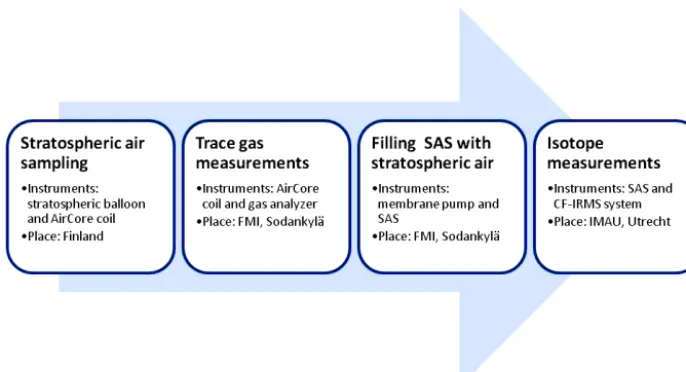
The stratospheric air samples are collected in a two-step pro-cedure. First, air samples from the surface up to the ceiling altitude of a stratospheric balloon flight (typically 30 km) are obtained with an AirCore system. Second, the stratospheric part of the collected air samples is recovered into an SAS af-ter online analysis of trace gas concentrations. The details of the first step (Chen et al., 2016) are here briefly described in Sect. 2.1. Section 2.2 and 2.3 provide the information relevant to the stratospheric air samples: the sub-sampling method and the description of the analytical system used for CO2 isotope measurement. We include a schematic
il-lustration for describing all the instruments and procedure in Fig. 1.
2.1 Stratospheric air sampling with AirCore
The AirCore device is made of stainless steel tubing coated with SilcoNert®1000 and has a total length of 100 m (40 m at 1/4 inch and 60 m at 1/8 inch, with a wall thick-ness of 0.01 inch). The payload that includes the AirCore and a radiosonde (Vaisala, type RS92-SGPL) weighs about 3.6 kg. Before each flight the AirCore is filled with a stan-dard dry fill-gas with known CO2, CH4 and CO mole
fractions (CO2=386.10±0.09 ppm; CH4=1880±2 ppb;
CO=7972±5 ppb) and closed with a shut-off valve at the inlet (Swagelok, part number SS-1GS4). A stratospheric bal-loon (Totex, type Tx3000) is used to launch the payload high into the stratosphere near Sodankylä, Finland. Just before launching the AirCore, the shut-off valve is opened, so that during the ascent the fill-gas leaves the AirCore coil due to the drop in pressure. After reaching an altitude of approxi-mately 30 km, the balloon bursts, and the descent of the pay-load on a parachute begins. Ambient air flows into the Air-Core and the air from higher altitudes is continuously com-pressed and pushed towards the closed end of the AirCore by air from lower altitudes. The shut-off valve is closed au-tomatically about 10 s after the landing, and the AirCore is quickly recovered and transported to the Finnish Meteoro-logical Institute (FMI) laboratory for analysis.
2.2 Sub-sampling into SAS
The vertical profiles of CO2, CH4and CO mole fractions are
Figure 1.A schematic diagram showing the overall procedure described in this work, from AirCore sampling on the site to IRMS analysis in laboratory.
Figure 2.Schematic diagram of the analytical system for trace gas analyses with a Picarro instrument and for transferring the air from the AirCore coil into the Stratospheric Air Sub-Sampler (SAS). The three-way valves in the SAS are in “open to the right” position when the AirCore air is transferred into the SAS and closed after sub-sampling. The crossed circles are conventional valves. The open circles at the inlet of the fill-gas and the calibration-gas cylinder represent cylinder valves and pressure regulators. The black circle represents the shut-off valve at the end of the AirCore coil. The drying tube is filled with magnesium perchlorate (Mg(ClO4)2) from Sigma-Aldrich.
outlet of Picarro instrument and set to 38.2 mL min−1.
Cal-ibration air can be analysed before and after measurement of the AirCore air. After the trace gas analysis, the top (i.e. stratospheric) part of the air collected with the AirCore (less than 20 % of the total collected air) is transferred into an SAS that is sent to Utrecht University for CO2isotope analysis.
into the inlet of the Picarro analyzer and then connected the outlet of the pump to the inlet of the Picarro analyzer. Thus a closed loop without the SAS was established, and the CO2
spike was measured multiple times as it circulated through the analyzer and the pump. This experiment allowed us to determine the timing of air travelling from the inlet of the analyzer to the inlet of the SAS. The flow rate was measured with a flow meter, and the timing for the sub-sampling pro-cedure was established. Also, the membrane pump (Picarro Inc.) that is used for the sub-sampling was carefully tested for leaks to avoid contamination of stratospheric air with ambi-ent laboratory air during the sub-sampling process. The out-let of the pump was connected to the gas analyzer (Picarro Inc., model G2401-m) to form a closed loop, which was filled with air with high mole fractions of CO2, CO and CH4. The
flow rate was set to 35 mL min−1and the air enclosed in this closed system was circulated nine times while measuring the CO2, CO, CH4and H2O mole fractions. The CO2mole
frac-tions stayed between 940.4 and 941.0 ppm and a small initial fluctuation quenched after nine cycles. The rate of change of CO2mole fraction based on these measurements with a very
high CO2mole fraction difference between the sample and
ambient air was 0.1 ppm of CO2 per minute. The effect of
such a small contamination on the isotopic composition of CO2is therefore negligible (<0.001 ‰ given the maximum
117O(CO2) of 5 ‰; see below). We note, however, that CO
gets contaminated in the sub-sampling process at a rate of 17 ppb min−1for CO (from a starting value of 500 ppb), so CO measurements would be compromised.
The SAS used for the CO2 isotope measurements in
Utrecht is made of 10 2 m long pieces of 1/4 inch diameter stainless steel tubing, which are connected by 11 Swagelok valves (part number SS-3CXS4) to form the 20 m long SAS. The tubes are bent to form identical rings to facilitate easy handling and transport. In the following, we refer to the rings as “SAS segments” and the valves as “three-way valves”. The three-way valves are open and connect the segments when the stratospheric part of the AirCore air fills the SAS and are kept closed when the sub-sampling process is fin-ished. Each SAS segment contains about 25 mL of the Air-Core air. Segment 1 corresponds to the highest altitude of the AirCore flight, and segment 10 contains air from the lower-stratosphere.
The idea of the SAS that is described here in detail has already been successfully implemented to enable the radio-carbon analysis of stratospheric CO2at the Centre for Isotope
Research in Groningen, the Netherlands (Paul et al., 2016).
2.3 Continuous flow system to measure the isotopic
composition of CO2
The analytical system to measure the isotopic composition (δ13C, δ18O and 117O) of CO2 in each SAS segment is
based on the principle presented in Mrozek et al. (2015). The isotopic composition is measured after gas
chromato-graphic separation of the CO2 from other air constituents.
The 17O content cannot be determined directly from the measurement atm/z=45, because of the isobaric interfer-ences of13C and17O. Therefore, the17O content is obtained from isotope measurements on CO2before (PreCO2) and
af-ter oxygen isotope exchange (PostCO2) with a large
reser-voir of oxygen. Instead of using cerium (IV) oxide (CeO2)
as exchange material (Assonov and Brenninkmeijer, 2001; Mrozek et al., 2015), we use in our new system copper ox-ide (CuO) (Kawagucci et al., 2005). A single measurement requires two independent injections of 1 mL of air: one for direct measurement (PreCO2) and one for measurement after
oxygen isotope exchange (PostCO2), plus 0.7 mL for
flush-ing the injection lines (all at 1 bar pressure). To reduce the measurement uncertainty statistically we perform multiple measurements on one air sample.
In addition to the requirement of overpressure in the in-jection unit, another disadvantage of the method presented in Mrozek et al. (2015) was the severe peak broadening that was introduced by the strong flow resistance of the CeO2
pow-der in the oxygen exchange unit, which required re-focusing of the CO2 after equilibration. In the new system the
pow-dered CeO2in the oxygen exchange unit was replaced with
CuO wires. As a result the peak broadening was dramati-cally reduced by a factor of 7.5 (from 450 to 60 s) and the equilibrated CO2could be analysed without re-focusing. In
addition, we developed a custom-made sample injection unit for samples provided by the SAS, where both sample and reference gas are injected via the SAS.
The improved continuous flow isotope ratio mass spec-trometry analytical system (CF-IRMS) analytical system consists of: a sample injection unit to attach the SAS seg-ments, a gas chromatographic column to separate the CO2
from a 1 mL air aliquot, an oxygen isotope exchange unit for CO2equilibration with CuO and open split interface and
an IRMS for isotope measurement (Fig. 3). Similar to the method described by Mrozek et al. (2015), three 6-port, 2-position Valco valves (VICI, C6UWM) direct the gas flows through the analytical system. The four main components are described in the following subsections.
2.3.1 Sample injection
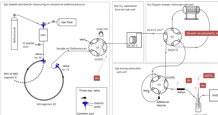
Figure 3.Schematic diagram of the CF-IRMS analytical system for complete isotope analysis (including117O) of stratospheric CO2. The
system is divided into four units:(a)sample injection,(b)gas chromatographic column (GC) to separate CO2from air and N2O,(c)optional oxygen isotope exchange unit and(d)isotope detection unit including open split interface and isotope ratio mass spectrometer (IRMS). MFC is mass flow controller, V1–V3 are Valco valves, RefCO2is Utrecht working reference CO2, the crossed circles are conventional valves
and the blue T’s are the three-way valves. The SAS three-way valves are normally closed but here they are shown in the sample admission position.
A single117O(CO2) measurement requires two
indepen-dent injections of the sample gas. The first injection is used for direct isotope measurement of CO2 (PreCO2), the
sec-ond injection is for measuring the isotopically equilibrated CO2(PostCO2). We inject the gas (reference air or sample
air) into the GC column via a 1 mL sample loop in V1. The sample loop is always filled to ambient pressure because it is open to the outside air via the vent. We use extended flushing during sample loop loading (the 1 mL sample loop is flushed with the sample gas at a flow rate of 1 mL min−1for 80 s) to avoid interference from outside air that may diffuse through the vent tubing into the sample loop.
It takes less than 1 h to measure an individual SAS seg-ment, however, in the present set-up reference air is mea-sured for several hours between the different segments (see Sect. 2.4.2). Usually two SAS segments are measured in one day. The CF-IRMS system operates fully automated and the only manual step required is the connection of the segments.
2.3.2 CO2separation from air
This sub-unit consist of a gas chromatography (GC) capillary column (ParaPLOT Q 25 m×0.53 mm, Varian). As a carrier we use helium at a flow rate of 4 mL min−1, supplied to the GC through one of the ports in valve V1. The GC is kept in-side a heated stainless steel box at 40◦C to ensure uniform conditions for gas separation. On the GC column the
differ-ent air constitudiffer-ents are separated. The air peak (mainly O2
and N2) elutes at 120 s after sample injection, CO2at 160 s
and N2O at 190 s. The air peak leaves the analytical system
through the vent in valve V3. Both CO2and N2O are directed
either to IRMS or to the isotope exchange sub-unit. Nitrous oxide in our system does not interfere with CO2during the
isotope ratio measurement because it is fully separated from CO2and gets destroyed in the CuO oven. This is discussed
in detail in Sect. 3.1.
2.3.3 Oxygen isotope exchange with CuO
This sub-unit consists of Valco valve 2 (V2) and an optional oxygen equilibration oven, the same as (Mrozek et al., 2015). The Valco valve V2 directs the CO2aliquot either directly
to the IRMS or first into the equilibration oven before en-tering IRMS. The oven is an assembly of a quartz glass reaction tube (1.4 mm i.d., 3.0 mm o.d., 300 mm length), a tube furnace and a temperature controller. Inside the tube there are oxygenated Cu wires and a Ni catalyst. We refer to this assembly as CuO oven. At a temperature of 900◦C, the wires act as a fast and highly efficient oxygen equilibration medium. This is similar to Kawagucci et al. (2005), who for the same purpose used twisted wires of CuO and Pt catalyst, and different from (Assonov and Brenninkmeijer, 2001) and Mrozek et al. (2015), who used CeO2powder. The important
in our system is the much smaller flow resistance. There-fore, the new exchange unit induces a much smaller peak broadening, and the equilibrated CO2does not require
focus-ing anymore. As a result, the sfocus-ingle analysis time shortened by 250 s in comparison to the method described in (Mrozek et al., 2015) (650 s instead of 900 s) and no liquid nitrogen is required.
Before first use, and then on a weekly basis, the CuO oven is conditioned with O2(Ultra High Purity (UHP), Air
Prod-ucts) at a flow rate of 20 mL min−1 and a temperature of 600◦C, following the procedure of (Kawagucci et al., 2005). Under these conditions, the copper metal forms a coating of copper (II) oxide on the surface of the Cu wires according to Cu+1
2O2→CuO. (R1)
After oxygenation, the IRMS needs at least 50 ments for the signal to stabilize. During routine measure-ments we monitor theδ18O(CO2) RefAir vs. VSMOW signal
before and after equilibration to make sure that the equilibra-tion reacequilibra-tion is quantitative.
2.3.4 IRMS interface and mass spectrometric analysis
This sub-unit of the analytical system (Fig. 3d) consists of a Valco valve 3 (V3), a Nafion™ dryer, a custom-made open split system (Röckmann et al., 2003) and an IRMS (Thermo Fisher Scientific Delta V Advantage). The loop in valve V3 is used to insert an additional volume of approximatively 1 mL volume (1/4 inch o.d. tube connected with Swagelok fittings) into the flow path, which smooths and ensures a compact shape of the PostCO2peak in the IRMS. The Nafion dryer
re-moves traces of water before the gas stream enters the IRMS via the open split system, which is also used to inject the pure CO2working gas. The IRMS measures ion current
ra-tios 45/44 and 46/44 that originate from CO2isotopologues
with masses 44, 45 and 46.
2.3.5 Reference air and reference CO2
Our reference air cylinder (referred to as RefAir in the following) was filled with tropospheric air collected at an altitude of 20 m from the sixth floor of the Buys Bal-lot building on the Utrecht University campus in July 2014. The isotopic composition of the CO2 in the
refer-ence air cylinder was calibrated against air cylinders pro-vided by an intercomparison program of the World Mete-orological Organization (WMO) and assigned the follow-ing isotope values:δ13CRefAir/VPDB= −8.09±0.10 ‰ and
δ18ORefAir/VSMOW=41.05±0.20 ‰. Following a mass
de-pendent fractionation relation of tropospheric CO2(Kaiser,
2009), we assign δ17ORefAir/VSMOW=21.5 ‰, so that
117ORefAir=0.0 ‰. The isotopic composition of the
refer-ence air is measured continuously in between the samples to monitor the stability and to correct for long-term trends of the CF-IRMS system.
The δ values for the working reference CO2 that is injected via the open split
sys-tem are δ13CRefCO2/VPDB= −36.16±0.01 ‰ and
δ18ORefCO2/VSMOW=4.69±0.01 ‰.
2.4 Measurement procedure
2.4.1 Connecting the sub-sampler to the continuous
flow isotope analysis system
We start the CO2isotope analysis always from the SAS
seg-ment with the highest segseg-ment number, here segseg-ment number 10. The common port of valve no. 11 (the end of segment 10) is connected to the injection line, which leads to V1, and the free port of valve no. 10 (the beginning of segment 10) to the MFC delivering reference air (see Fig. 3). Note that the beginning of the segment 10 is also the end of segment 9.
The injection lines are open to the laboratory air when the SAS segments are being exchanged. To avoid mixing of the precious sample air with laboratory air we evacuate the vol-ume between the MFC and the SAS segment with the LV pump and flush this volume with reference air (LV pump ex-changed to vent). It is important to depressurize the volume behind the MFC before opening the SAS segment. Overpres-sure in the injection lines must be avoided so that the small air sample is not pushed out of the inlet system.
After connecting an SAS segment as described above, the three-way valve no. 10 is opened, so that reference air starts slowly flowing through segment 10. Next, the three-way valve no. 11 is opened, so that air is flushed to the sample loop of the injection system (see Fig. 3). The sample admis-sion procedure is described in detail in the next section.
As the sample air is flushed into the system by the refer-ence air, we simply continue measuring the referrefer-ence air that is then flowing through the SAS segment. A disadvantage is that the last injections of the sample air are actually a mix-ture of sample and reference air (see below). The measure-ments of reference air after the sample measurement are later used for referencing. After the reference air measurements are completed, we close the three-way valves and disconnect segment 10. As the common port of valve no. 10 has to be connected to the injection line when measuring segment 9, segment 10 has to be physically disconnected from the SAS. Segment 9 is then treated the same as segment 10 before. We continue measuring and exchanging SAS segments one by one.
2.4.2 Isotope analysis procedure
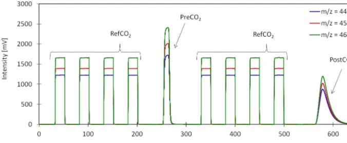
Figure 4. Example of a typical IRMS chromatogram of a single 117O(CO2) analysis with the CF-IRMS system described here. The
eight square peaks are the working reference CO2(RefCO2) peaks injected directly via the open split interface. The non-equilibrated CO2
(PreCO2) peak and the equilibrated CO2(PostCO2) peak are the two sample gas peaks.
15 s before opening the SAS valve in order to provide a small and reproducible overpressure at the entrance of the SAS seg-ment. We then open the three-way valve towards the SAS segment to admit the reference air from the MFC, and 1 s later the three-way valve before V1. Now, the flow of refer-ence air pushes the AirCore air towards the sample loop in V1. It takes 10 s for the AirCore air to travel from the SAS segment to the sample loop and another 80 s to fill it. At 80 s, the flow rate at the MFC is stopped to save sample and the air is allowed to further expand into and fill the injection loop. At 90 s the loop is fully filled and Valco valve V1 is switched for 40 s to position INJECT to transfer the first aliquot of the sample air into the analytical system. The 1 mL aliquot of air from the SAS segment is transferred to the GC column in a He carrier gas (4 mL min−1). In the GC column, the CO2
is separated from other atmospheric gases. All compounds are directed via Valco valve V2 (INJECT) and Valco valve V3 (LOAD) directly towards the isotope detection unit. The CO2 is injected into the ion source of the IRMS (PreCO2),
all other gases are discarded via the open split.
As soon as the CO2peak (PreCO2) appears on the
chro-matogram, the second aliquot of the AirCore air is introduced into the system. Similar to the first injection, the sample loop is flushed with the AirCore air for 80 s (MFC is set to a flow rate of 1 mL min−1between 290 and 370 s). At 380 s valve V1 is switched for 40 s from LOAD to INJECT, and the sec-ond aliquot of the AirCore air is injected into the GC col-umn. Non-CO2gases leave the analytical system through the
open split capillary between 500 and 520 s (V2 in position INJECT and V3 in position LOAD). At 545 s, V2 switches to position LOAD, and the CO2is directed to the isotope
ex-change unit. After the isotope exex-change reaction, the equili-brated CO2(PostCO2) is flushed further to V3. An additional
1 mL stainless steel volume in front of Valco valve V3 has been added to smoothen the peak shape of the equilibrated CO2 (PostCO2), leading to improved precision. The
equili-brated CO2 is detected on the chromatogram between 560
and 640 s.
Figure 4 presents an example of an IRMS chromatogram. A single measurement including two injections takes 650 s. The CO2 peak from the first injection (PreCO2) is detected
between 250 and 280 s, and the equilibrated CO2peak from
the second injection (PostCO2) between 560 and 640 s. The
eight working reference CO2peaks (RefCO2) are injected to
the IRMS directly via the open split interface: four before detection of the PreCO2(0–200 s) and four before detection
of the PreCO2(300–500 s). The two sample peaks (PreCO2
and PostCO2) have a different shape because the second one
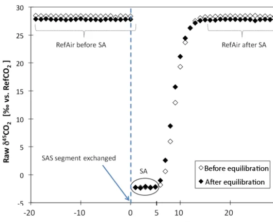
has passed the exchange unit and the additional volume. For each SAS segment we run a sequence of 35 individual measurements (of two injections each). The results show that 5 of these measurements represent pure sample gas (SA), 10 of them contain sample-reference air mixtures, and 20 are pure reference air (RefAir) measurements (see Fig. 5). Theo-retically, we should be able to analyse nine SA aliquots from each SAS segment (25/2.7 mL), but as described above the reference air is used as carrier gas and mixes with the sample air. Since we know the isotopic composition of the reference air, the method can potentially be improved by extracting SA information also from the “mixed” SA/RefAir peaks, which may decrease measurement uncertainty statistically (see Ta-ble 1).
3 Performance of the continuous flow isotope analysis
system
3.1 Separation and destruction of N2O
Nitrous oxide (N2O) interferes with the mass spectrometric
analysis of CO2because the isotopologues of both CO2and
N2O fall on the mass 44, 45 and 46 collectors and cannot be
Figure 5.Raw-δ45CO2data (‰ vs RefCO2) from a complete measurement sequence of an SASsegment. SA is the air sample stored in the SAS segment. RefAir before SA refers to the reference air passing through an empty SAS segment and defines IRMS stability before the new SA is connected. After exchanging the SAS segments we obtain five “pure” sample air measurements. Subsequent to the SA measurement, the reference air first mixes into the sample air; it takes about 10 measurements until pure reference air is processed. RefAir after SA refers to the reference air passing through the SAS segment after the SA has been completely flushed out. For the sample air presented here the “before equilibration’ points overlap with the “after equilibration” points and cannot be distinguished.
Table 1.Statistical improvement of117O analytical error by combining multiple (n) measurements of the same gas into packages and taking the standard error of these packages.
Test group Number of packages Number of measurements Random error SE theoretical: SE experimental: name in the group in the package: (n) factor: 1/√(n) SD/√(n) SD over117O mean/√(n)
A 1 270 0.061 0.074
B 2 135 0.086 0.105 0.205
C 3 90 0.105 0.129 0.256
D 5 54 0.136 0.166 0.170
E 6 45 0.149 0.182 0.245
F 9 30 0.183 0.223 0.251
G 10 27 0.192 0.235 0.302
H 15 18 0.236 0.288 0.316
I 18 15 0.258 0.315 0.345
J 27 10 0.316 0.386 0.405
K 30 9 0.333 0.407 0.472
L 45 6 0.408 0.498 0.531
M 54 5 0.447 0.546 0.570
N 270 1 1.000 1.220 1.220
The bold values describe the uncertainty for a single measurement and the error expected for the five repeated measurements on one air sample stored in the SAS. SD: standard deviation.
significant analytical biases forδ13C(CO2),δ17O(CO2) and
δ18O(CO2) values and, as result, decrease117O of
strato-spheric air by as much as 3 ‰ (Wiegel et al., 2013). Note that N2O and CO2can also not be separated cryogenically
(Mook and Jongsma, 1987).
To measure CO2 isotopes in an air sample without
inter-ference from N2O we completely separate N2O from CO2
before the isotope ratio analysis on the GC column (Ferretti et al., 2000). In addition, for the measurement of PostCO2,
Figure 6.IRMS chromatogram demonstrating the separation of N2O from CO2on the GC column and the absence of an N2O peak after the
hot CuO/Ni isotope exchange unit. The artificially prepared mixture of N2O and CO2was injected to the analytical system following the procedure described in Sect. 2.4.2. In order to observe the N2O peak the fifth working RefCO2peak was omitted in the chromatogram and
the measurement time was extended to 750 s.
unit (Kawagucci et al., 2005; Assonov and Brenninkmeijer, 2006; Mrozek et al., 2015).
To demonstrate successful GC separation and N2O
decom-position inside the CuO oven at 900◦C we connected a dilu-tion of 400 ppm N2O in synthetic air to the injection sub-unit
of our analytical system. The N2O enriched gas was placed
at the position of a flask, as shown in Fig. 3. The flask was opened and the N2O enriched gas filled the injection lines
and the 4 mL inner volume of MFC. Next, we changed the position of the three-way valve in front of the MFC so that the reference air was flowing towards the MFC. As a conse-quence, the reference air mixed with the N2O-rich gas and
both N2O and CO2 were observed on the chromatogram.
We monitored the N2O peak before and after the isotope
ex-change reaction: for the non-heated aliquot, the GC column separated completely the N2O from the CO2; for the heated
aliquot, the N2O was destroyed completely in the CuO oven
(see Fig. 6). For the experiment shown in Fig. 6, the chro-matogram was extended to 750 s instead of the normal length of 650 s because N2O elutes after CO2. Additionally, the fifth
working RefCO2peak was omitted in order to observe the
N2O peak. The test shows that N2O can be effectively
re-moved on CuO/Ni wires at 900◦C and confirms the results of (Kawagucci et al., 2005). This removal method can poten-tially be applied to other trace gas measurement techniques.
3.2 CuO–CO2equilibration efficiency
To quantify the efficiency of oxygen isotope equilibration in the CuO oven we analysed two samples containing CO2
with very different isotopic composition. The first one was our RefAir and the second one was a synthetic mixture of RefCO2diluted to 400 ppm CO2 in synthetic air. The
sam-ples were injected via a stainless tube that is similar to a segment of the SAS, but longer (4 m length 1/4 inch o.d.). First, the reference air was injected multiple times through this tube. Next, we filled the injection tube with the RefCO2
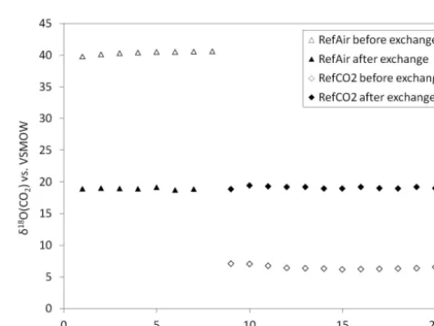
dilution and continued the measurements. Figure 7 presents
Figure 7.Efficiency of oxygen isotope equilibration in the CuO oven. Theδ18O(CO2) values of RefAir and a mixture of RefCO2 in synthetic air are shown before and after isotope equilibration. The last point of the RefAir measurement sequence after exchange is missing because the peak of the last run was accidentally not registered.
the results. The isotopic difference between the two CO2
samples was about 36 ‰ before isotope exchange. After the isotopic exchange reaction both gases were equilibrated to δ18O=(19.03±0.18) ‰. From the difference in the oxy-gen isotopic composition between RefAir and RefCO2
di-lution before and after oxygen isotope exchange, the oxy-gen exchange efficiency in CuO oven was calculated to be >99.5 %. We conclude that the oxygen exchange reaction with CuO/Ni wires at 900◦C is complete.
3.3 Error analysis
of reference air were injected continuously to the CF-IRMS system for 50 h, comprising 270 individual measurements of the complete isotopic composition of CO2. The standard
deviation of 117O(CO2) over all 270 measurements was
1.22 ‰. This is the error that we assign to a single mea-surement with the new analytical system. In our previously published method (Mrozek et al., 2015), the 117O(CO2)
standard deviation in such a long-term stability test was 1.68 ‰. The improvement compared to the system described in (Mrozek et al., 2015) is due to the replacement of the isotope exchange medium from powdered CeO2 to CuO
wires and through abandonment of a liquid nitrogen trap for re-focusing of the isotopically equilibrated CO2. For
δ18O(CO2) and δ13C(CO2) the standard deviation over all
270 measurements was 0.06 and 0.07 ‰, respectively, vs. 0.16 and 0.09 ‰ in (Mrozek et al., 2015).
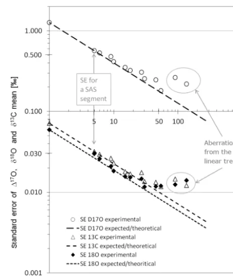
To investigate how the measurement error is reduced sta-tistically with multiple measurements on an air sample, we divided the 270 measurements from the stability test into dif-ferent packages of nnumbers of measurements (two pack-ages of 135 measurements each, three packpack-ages of 90 mea-surements each, etc.). The experimental standard error (SE) for each set of packages was then compared to the the-oretically expected error. Calculations for 117O(CO2) are
shown in Table 1; the results for 117O(CO2), δ18O(CO2)
andδ13C(CO2) are displayed in Fig. 8. Since the SE is
de-fined asσ/n0.5the expected slope on this double logarithmic plot is −0.50. The error reduction follows the theoretically expected relation quite well. When the two groups with only two and three members each are neglected, the linear fit to the data has a slope of−0.46±0.02 for117O,−0.42±0.03 forδ18O and−0.45±0.03 forδ13C. Within the error, this is close to the theoretical slope of−0.50.
We conclude that repeated measurements on one air sample (up to 54 repetition that corresponds to 2.6 µmol CO2) can reduce the uncertainty in117O(CO2) to 0.2 ‰.
More than 54 repetitions on one air sample improves the 117O(CO2) uncertainty only marginally. This uncertainty is
in the same range as previously reported techniques for large samples, most of which did not allow the measurement of very small samples. (Bhattacharya and Thiemens, 1989) re-ported an uncertainty of 0.1 ‰ using a BrF5-based technique,
(Brenninkmeijer and Röckmann, 1998) obtained 0.2 ‰ with a two-step fluorination method, (Assonov and Brenninkmei-jer, 2001) reported 0.33 ‰ with a CeO2 exchange method
and (Mahata et al., 2012) improved this method to an un-certainty of 0.12 ‰. The (Kawagucci et al., 2005) method is the only technique that also targeted very small sample sizes (like our system) and they reported an uncertainty of 0.35 ‰. For five repeated measurements on one stratospheric air sample stored in the SAS (an example of a CF-IRMS mea-surement sequence is given in Fig. 5) we therefore expect an uncertainty of 0.57 ‰ for117O(CO2) and 0.03 ‰ for both
δ18O(CO2) andδ13C(CO2). This will be compared to the
re-producibility of the actual SAS measurements in Sect. 4.2.
Figure 8.Correlation of ln(SE) vs. ln(n) for117O(CO2) (based
on data from Table 1),δ18O(CO2) andδ13C(CO2). SE is the
stan-dard error of the mean, and n is the number of measurements in a package. The experimental SE of 117O, δ18O and δ13C are shown as circles, triangles and black diamonds respectively. The dashed/dotted lines are the theoretically expected slopes for the linear correlation between ln(SE) and ln(n). For a packages ofn≤54, the experimentally derived slopes are−0.46±0.02 for 117O,−0.42±0.03 forδ18O and−0.45±0.03 forδ13C. The val-ues are close to the theoretical slope of−0.50 (dotted/dashed lines). Based on this experiment we expect an uncertainty of±0.57 ‰ for 117O of an AirCore air sample stored in an individual SAS seg-ment.
4 AirCore flight on 5 November 2014
Figure 9.Stratospheric CO2mole fraction profile for an AirCore descent near Sodankylä, Finland (67◦N), in November 2014, as a function
of altitude (km) and pressure (mbar). The numbers and the various line styles indicate the sub-sampler segments into which the respective part of the air from the AirCore coil was transferred after the trace gas analysis. The general trend of the profile agrees with the already published data (Foucher et al., 2011). The distribution of the air sample in the SAS segments is proportional to the pressure change during the AirCore descent: here 16 mbar per SAS segment.
stratospheric air was transferred into the SAS. The SAS was sent to the laboratory in Utrecht for CO2isotope analysis.
4.1 Assigning the trace gas data to the SAS segments
We assigned the trace gas mixing ratios measured with the Picarro instrument to the individual SAS segments based on the flow rate of the carrier gas and the time required to fill the SAS. As the SAS has 10 segments, the air in each seg-ment represents 38.6 s of trace gas measureseg-ments with the Picarro instrument. The second piece of information that is necessary for correct assignment is the starting time for the sub-sampling. This starting time was established by taking into account the transfer time of air from the outlet of the Pi-carro analyser to the inlet of the SAS and the time required to flush out the initial portion of fill-gas from the AirCore. To ensure that no fill-gas was transferred into the SAS, the top fraction of the stratospheric air (which immediately fol-lows the fill-gas) also had to be discarded. This way we lost the stratospheric air from above 25 km. The timing of sub-sampling has in the meantime been improved to discard less stratospheric air in future samplings.
Figure 9 shows which part of the stratospheric AirCore air is stored in which segment of the SAS, both as function of altitude and pressure. Note that the SAS segments are equally spaced in pressure change (here 16 mbar/segment) during the descent rather than altitude. For example, the SAS segment 1 contains air from 24.5 to 21.4 km, while the SAS segment 2 contains air from 21.4 to 19.2 km. An analysis of the trace gas profiles from the AirCore flight will be published separately.
4.2 117O(CO2) analysis of the AirCore air stored in the SAS
The stratospheric part of the AirCore air from 5 November 2014 flight was measured in Utrecht between 25 November and 1 December 2014. The results showed that segments 10 and 8 were contaminated with CO2from outside air. The
pre-cise origin of this contamination could not be determined, but it could have happened when connecting SAS segments to the injection sub-unit of the CF-IRMS system. Due to an accidental instability in the helium carrier gas flow, the air sample from the SAS segment 6 was lost.
As shown in Fig. 5, we were able to perform five re-peated CF-IRMS measurements on the other seven strato-spheric air samples stored in SAS. The average (1σ) stan-dard deviation of the raw molecular mass ratios (45/44 and 46/44) of an air sample was 0.04 and 0.02 ‰ for non-equilibrated CO2and 0.07 and 0.11 ‰ for equilibrated CO2
respectively. The main contribution to the measurement error of117O is the uncertainty in the isotope ratio 45/44 (Bren-ninkmeijer and Röckmann, 1998). Based on the reproducibil-ity of m/z 45 of equilibrated and non-equilibrated CO2 ( p
(0.04)2+(0.07)2×15), the uncertainty inδ17O for a
sin-gle measurement was 1.25 ‰ and for a package of five mea-surements it was 0.56 ‰ (1.25 ‰/
√
Figure 10.Comparison of the linear negative correlation between117O(CO2) and N2O from measurements of the AirCore/SAS samples (red rhombuses) presented here with literature data from (Kawagucci et al., 2008) (blue crosses) and (Wiegel et al., 2013) (black triangles). For the AirCore dataset, N2O mole fractions were deduced from CH4mole fractions as described in the text. The horizontal error bars are a combination of the range of CH4mole fractions that is combined within a single SAS segment and the error of the CH4–N2O transfer
function. The vertical error bars represent117O(CO2) uncertainty of 0.56 ‰ (1σ).
package of five repeated analyses from an SAS segment. This is again very similar to the expected error from the long-term stability test as presented in Fig. 8.
4.3 117O(CO
2)–N2O correlation
The mole fraction of N2O is a good tracer for the
photo-chemical processing of long-lived trace gases in the strato-sphere (Park et al., 2004; Kaiser et al., 2006). Nitrous oxide was not measured in the AirCore air, but CH4was measured
and we use the relationship between stratospheric CH4and
N2O mole fractions at high latitudes to translate the CH4
mole fractions to N2O mole fractions. For this purpose we
used CH4–N2O data from two cryosampler flights in the
Arc-tic in 2009 and 2011 (Engel et al., 2016). The fit function for the CH4–N2O dataset was provided to us by Andreas
Engel, Goethe University Frankfurt, Germany. The strato-spheric pseudo-N2O profile derived this way was then
av-eraged according to the 10 individual SAS segments. A de-tailed discussion on obtaining N2O mole fractions from the
measured CH4 will be provided together with the scientific
interpretation of the data in Mrozek et al. (in prep.).
In Fig. 10 we show the N2O mole fractions deduced from
the CH4 profile vs. the117O(CO2) data of the AirCore air
samples analysed from the SAS. The linear negative correla-tion between N2O and117O(CO2) is well known from
pre-vious studies and was discussed before (Boering et al., 2004; Kawagucci et al., 2008; Wiegel et al., 2013). Here, we use
this correlation as an additional, independent check on the system calibration. The AirCore air samples agree with the already published data, suggesting that our measurements are well calibrated. The scatter of our data is similar to the vari-ability of the data presented by Kawagucci et al. (2008). The data presented by Wiegel et al. (2013) show smaller vari-ability, but our measurements were obtained from samples of 25 mL of air at ambient pressure only; this is up to 80 times smaller sample size than used in the measurements of Wiegel et al. (2013). The variability of our data around the linear fit is within the analytical uncertainty of 0.56 ‰ (1σ) per SAS segment. The uncertainty of the N2O mole fraction
in Fig. 10 reflects the standard deviation of the N2O
pro-file stored in an individual SAS segment. It is up to 20 ppb (1σ) for the high-altitude AirCore air samples where N2O
showed a strong trend and 2 ppb (1σ) for lower altitude sam-ples where N2O is more constant. The complete CH4, CO
and CO2mole fraction dataset and in-depth analysis on CO2
isotope measurements from the 5 November 2014 AirCore flight over Sodankylä, Finland, will be published separately. We conclude that air sampling with an AirCore, followed by sub-sampling of stratospheric air in 10 segments of the SAS and analysis with the analytical system described here provides a relatively cost-effective technique for obtaining vertical profiles of the complete isotopic composition of CO2
stratospheric profile of the AirCore air after online analysis is preserved and the individual sub-samples can be supplied to relatively slow analytical instrumentation. The SAS is easy to construct and simple to use, also in the field.
To illustrate the scientific possibilities, the SAS was cou-pled to a continuous flow analytical system for measurement of the 17O excess of CO
2. The air from the SAS was
sup-plied via a new sample introduction system to allow isotope analysis on very small samples. The sample injection occurs at ambient pressure and we use the reference air as the car-rier gas. The determination of117O of CO2is performed by
measuring CO2before and after complete oxygen isotope
ex-change with a large oxygen reservoir provided by CuO/Ni. The standard error for a 25 mL air sample at stratospheric CO2 mole fraction is 0.56 ‰ (1σ) for 117O and ‰ (1σ)
for bothδ18O andδ13C. The analytical system operates free of liquid nitrogen because the isotopically equilibrated CO2
does not require a focusing step, unlike the (Mrozek et al., 2015) method.
The concept of SAS and its coupling to the analytical sys-tem for measurement of 117O was validated through mea-surements on stratospheric air samples obtained during an AirCore flight over Sodankylä, Finland, in November 2014. 117O shows the expected negative linear correlation with N2O, which provides an independent check on the system
calibration. In the future, we plan routine measurements of stratospheric profiles of117O together with the mole frac-tions of CO2, CH4and CO from AirCore flights on a regular
basis, which could expedite the use of the isotope signatures for studying stratospheric circulation patterns and reaction mechanisms. The concept of the SAS will further broaden the scientific questions that can be addressed by AirCore sound-ings (e.g. Paul et al., 2016).
6 Data availability
The datasets are available from https://www.projects.science. uu.nl/atmosphereclimate/Data.php (APCG, 2016).
Acknowledgements. This work was funded by the Marie-Skłodowska Curie ITN INTRAMIF (Initial Training Network in Mass Independent Fractionation) as a part of the European
References
Alexander, B., Vollmer, M. K., Jackson, T., Weiss, R. F., and Thiemens, M. H.: Stratospheric CO2isotopic anomalies and SF6
and CFC tracer concentrations in the Arctic polar vortex, Geo-phys. Res. Lett., 28, 4103–4106, 2001.
APCG: IMAU-APCG measurements data, available at: https: //www.projects.science.uu.nl/atmosphereclimate/Data.php, last access: 17 November 2016.
Assonov, S. S. and Brenninkmeijer, C. A. M.: A new method to determine the17O isotopic abundance in CO2using oxygen
iso-tope exchange with a solid oxide, Rapid Commun. Mass Sp., 15, 2426–2437, doi:10.1002/rcm.529, 2001.
Assonov, S. S. and Brenninkmeijer, C. M.: Reporting small117O values: existing definitions and concepts, Rapid Commun. Mass Sp., 19, 627–636, doi:10.1002/rcm.1833, 2005.
Assonov, S. S. and Brenninkmeijer, C. A. M.: On the N2O
correction used for mass spectrometric analysis of atmo-spheric CO2, Rapid Commun. Mass Sp., 20, 1809–1819,
doi:10.1002/rcm.2516, 2006.
Baertschi, P.: Absolute18O content of standard mean ocean wa-ter, Earth Planet. Sci. Lett., 31, 341–344, doi:10.1016/0012-821X(76)90115-1, 1976.
Bhattacharya, S. and Thiemens, M.: Oxygen Isotopic Fractiona-tions in Symmetry Dependent Chemical ReacFractiona-tions, in: Lunar and Planetary Science Conference, 20, p. 71, 1989.
Boering, K. A., Jackson, T., Hoag, K. J., Cole, A. S., Perri, M. J., Thiemens, M., and Atlas, E.: Observations of the anomalous oxy-gen isotopic composition of carbon dioxide in the lower strato-sphere and the flux of the anomaly to the tropostrato-sphere, Geophys. Res. Lett., 31, L03109, doi:10.1029/2003GL018451, 2004. Brenninkmeijer, C. A. M. and Röckmann, T.: A rapid method for
the preparation of O2from CO2for mass spectrometric
measure-ment of17O/16O ratios, Rapid Commun. Mass Sp., 12, 479– 483, 1998.
Chen, H., Kivi, R., Heikkinen, P.and Kers, B., de Vreis, M., Hatakka, J., Laurila, T., Sweeney, C., and Tans, P.: High-latitude balloon observations of CO2/CH4/CO using AirCore: evaluation of Sodankylä TCCON retrievals, in prep., 2016.
Ferretti, D. F., Lowe, D. C., Martin, R. J., and Brailsford, G. W.: A new gas chromatograph-isotope ratio mass spectrometry tech-nique for high-precision, N2O-free analysis ofδ13C andδ18O in atmospheric CO2from small air samples, J. Geophys.
Res.-Atmos, 105, 6709–6718, doi:10.1029/1999JD901051, 2000. Foucher, P. Y., Chédin, A., Armante, R., Boone, C., Crevoisier,
C., and Bernath, P.: Carbon dioxide atmospheric vertical pro-files retrieved from space observation using ACE-FTS solar occultation instrument, Atmos. Chem. Phys., 11, 2455–2470, doi:10.5194/acp-11-2455-2011, 2011.
IPCC 2013: Ciais, P., Sabine, C., Bala, G., Bopp, L., Brovkin, V., Canadell, J., Chhabra, A., DeFries, R., Galloway, J., Heimann, M., Jones, C., Le Quéré, C., Myneni, R., Piao, S., and Thornton, P.: Climate Change 2013: The Physical Science Basis. Contribu-tion of Working Group I to the Fifth Assessment Report of the Intergovernmental Panel on Climate Change, edited by: Stocker, T. F., Qin, D., Plattner, G.-K., Tignor, M., Allen, S. K., Boschung, J., Nauels, A., Xia, Y., Bex, V. and Midgley, P. M., Tech. rep., doi:10.1017/CBO9781107415324.015, 2013.
Kaiser, J.: Reformulated 17O correction of mass spectromet-ric stable isotope measurements in carbon dioxide and a critical appraisal of historic “absolute” carbon and oxygen isotope ratios, Geochim. Cosmochim. Ac., 72, 1312–1334, doi:10.1016/j.gca.2007.12.011, 2009.
Kaiser, J., Engel, A., Borchers, R., and Röckmann, T.: Probing stratospheric transport and chemistry with new balloon and air-craft observations of the meridional and vertical N2O isotope
dis-tribution, Atmos. Chem. Phys., 6, 3535–3556, doi:10.5194/acp-6-3535-2006, 2006.
Karion, A., Sweeney, C., Tans, P., and Newberger, T.: AirCore: An innovative atmospheric sampling system, J. Atmos. Ocean. Techn., 27, 1839–1853, doi:10.1175/2010JTECHA1448.1, 2010. Kawagucci, S., Tsunogai, U., Kudo, S., Nakagawa, F., Honda, H., Aoki, S., Nakazawa, T., and Gamo, T.: An analytical system for determining117O in CO2using continuous flow-isotope ra-tio MS, Anal. Chem., 77, 4509–4514, doi:10.1021/ac050266u, 2005.
Kawagucci, S., Tsunogai, U., Kudo, S., Nakagawa, F., Honda, H., Aoki, S., Nakazawa, T., Tsutsumi, M., and Gamo, T.: Long-term observation of mass-independent oxygen isotope anomaly in stratospheric CO2, Atmos. Chem. Phys., 8, 6189–6197,
doi:10.5194/acp-8-6189-2008, 2008.
Lämmerzahl, P., Röckmann, T., Brenninkmeijer, C. M., Krankowsky, D., and Mauersberger, K.: Oxygen isotope composition of stratospheric carbon dioxide, Geophys. Res. Lett., 29, 2–5, 2002.
Mahata, S., Bhattacharya, S. K., Wang, C.-H., and Liang, M.-C.: An improved CeO2method for high-precision measurements of 17O/16O ratios for atmospheric carbon dioxide., Rapid
Com-mun. Mass Sp., 26, 1909–1922, doi:10.1002/rcm.6296, 2012. Mook, W. G. and Jongsma, J.: Measurement of the N2O
correc-tion for13C /12C ratios of atmospheric CO2by removal of N2O,
Tellus B, 39B, 96–99, doi:10.1111/j.1600-0889.1987.tb00274.x, 1987.
Mook, W. G. and van der Hoek, S.: The N2O correction in the
car-bon and oxygen isotopic analysis of atmospheric CO2, Chem.
Geol., 41, 237–242, doi:10.1016/S0009-2541(83)80021-7, 1983. Mrozek, D. J., van der Veen, C., Kliphuis, M., Kaiser, J., Wiegel, A. A., and Röckmann, T.: Continuous-flow IRMS technique for de-termining the17O excess of CO2using complete oxygen isotope
exchange with cerium oxide, Atmos. Meas. Tech., 8, 811–822, doi:10.5194/amt-8-811-2015, 2015.
Park, S., Atlas, E. L., and Boering, K. A.: Measurements of N2O isotopologues in the stratosphere: Influence of transport
on the apparent enrichment factors and the isotopologue fluxes to the troposphere, J. Geophys. Res.-Atmos., 109, D01305, doi:10.1029/2003JD003731, 2004.
Paul, D., Chen, H., Been, H. A., Kivi, R., and Meijer, H. A. J.: Ra-diocarbon analysis of stratospheric CO2retrieved from AirCore
sampling, Atmos. Meas. Tech., 9, 4997–5006, doi:10.5194/amt-9-4997-2016, 2016.
Röckmann, T., Kaiser, J., Brenninkmeijer, C. A. M., and Brand, W. A.: Gas chromatography/isotope-ratio mass spectrometry method for high-precision position-dependent15N and18O mea-surements of atmospheric nitrous oxide., Rapid Commun. Mass Sp., 17, 1897–908, doi:10.1002/rcm.1132, 2003.
Thiemens, M., Jackson, T., Zipf, E. C., Erdman, P. W., and Egmond, V. C.: Carbon dioxide and oxygen isotope anomalies in the meso-sphere and stratomeso-sphere, Science, 270, 969–972, 1995.