Western Europe is warming much faster than expected

www.clim-past.net/5/1/2009/

© Author(s) 2009. This work is distributed under the Creative Commons Attribution 3.0 License.

Climate

of the Past

Western Europe is warming much faster than expected

G. J. van Oldenborgh1, S. Drijfhout1, A. van Ulden1, R. Haarsma1, A. Sterl1, C. Severijns1, W. Hazeleger1, and H. Dijkstra2

1_{KNMI (Koninklijk Nederlands Meteorologisch Instituut), De Bilt, The Netherlands} 2_{Institute for Marine and Atmospheric Research, Utrecht University, The Netherlands} Received: 28 July 2008 – Published in Clim. Past Discuss.: 29 July 2008

Revised: 22 December 2008 – Accepted: 22 December 2008 – Published: 21 January 2009

Abstract. The warming trend of the last decades is now so

strong that it is discernible in local temperature observations. This opens the possibility to compare the trend to the warm-ing predicted by comprehensive climate models (GCMs), which up to now could not be verified directly to observations on a local scale, because the signal-to-noise ratio was too low. The observed temperature trend in western Europe over the last decades appears much stronger than simulated by state-of-the-art GCMs. The difference is very unlikely due to random fluctuations, either in fast weather processes or in decadal climate fluctuations. In winter and spring, changes in atmospheric circulation are important; in spring and sum-mer changes in soil moisture and cloud cover. A misrepre-sentation of the North Atlantic Current affects trends along the coast. Many of these processes ontinue to affect trends in projections for the 21st century. This implies that climate predictions for western Europe probably underestimate the effects of anthropogenic climate change.

1 Introduction

Global warming has been detected in the global mean tem-perature and on continental-scale regions, and this warm-ing has been attributed to anthropogenic causes (Stott, 2003; IPCC, 2007). The observed global warming trend agrees well with predictions (Rahmstorf et al., 2007). However, cli-mate change projections are typically made for much smaller areas. The Netherlands, for instance, corresponds to a single grid box in most current climate models, but the temperature projections in the KNMI’06 scenarios (van den Hurk et al., 2006, 2007) are based on grid point values of global and re-gional climate models. In this region, temperatures simulated

Correspondence to: G. J. van Oldenborgh (oldenborgh@knmi.nl)

by Regional Climate models (RCMs) do not deviate much from GCMs, as the prescribed SST and boundary condition determine the temperature to a large extent (Lenderink et al., 2007).

By now, global warming can be detected even on the grid point scale. In this paper we investigate the high tempera-ture trends observed in western Europe over the last decades. First we compare these with the trends expected on the basis of climate model experiments. These turn out to be incom-patible with the observations over large regions of Europe. The discrepancy is very unlikely due to weather or decadal climate fluctuations (Smith et al., 2007; Keenlyside et al., 2008). Searching for the causes of the unexpectedly fast tem-perature rise in Europe, we discuss the differences between modelled and observed atmospheric circulation, ocean circu-lation, soil moisture and radiation, aerosols, and snow cover.

2 Data

deep water formation regions of the Labrador, Greenland, and Weddell Seas, and along the equator the meridional res-olution is about 0.5◦_{. There are 40 vertical layers with}

thick-ness ranging from 10 m at the surface to 600 m at the bottom. The experimental period is 1950–2100. For the historical part of this period (1950–2000) the concentrations of green-house gases (GHG) and sulphate aerosols are specified from observations, while for the future part (2001–2100) they fol-low SRES scenario A1b (Nakicenovic et al., 2000). This sce-nario has slightly higher CO2concentrations than observed in 2007. The runs are initialised from a long run in which historical GHG concentrations have been used until 1950. Different ensemble members are generated by disturbing the initial state of the atmosphere. Gaussian noise with an am-plitude of 0.1 K is added to the initial temperature field. The initial ocean state is not perturbed.

The findings from the ESSENCE ensemble are backed with results from ensembles from the World Climate Re-search Programme’s (WCRP) Coupled Model Intercompar-ison Project phase 3 (CMIP3) multi-model dataset. We use both a 22-model set (only excluding the GISS EH Model, which has very unrealistic results) and the subset of models with the most realistic circulation selected in van Ulden and van Oldenborgh (2006). The criterion used was that the ex-plained variance of monthly sea-level pressure fields should be positive for all months. The explained variance is given by

E=1−σ

2 diff

σ_obs2 (1)

Here,σ_diff2 is the spatial variance of the difference between simulated and observed long-term mean pressure, andσ_obs2 the spatial variance of the observed field. A negative ex-plained variance indicates that the monthly mean sea-level pressure deviates more from the observed field than the re-analysed field deviates from zero.

Apart from ECHAM5/MPI-OM, the models that were se-lected are the GFDL CM2.1 model (Delworth et al., 2006), MIROC 3.2 T106 (K-1 model developers, 2004), HadGEM1 (Johns et al., 2004) and CCCMA CGCM 3.2 T63 (Kim et al., 2002). Lower-resolution versions of these models also sat-isfy the criterion, but were thought not to contribute addi-tional information. Observed greenhouse gas and aerosol concentrations were used up to 2000, afterwards the SRES A1b scenario was prescribed.

Other metrics for the skill give different results. The corre-lation of evapotranspiration with downwelling radiation (an indication of soil moisture effects) influences summer tem-perature trends. The realism of this process selects against two of these models (Boe and Terray, 2008).

The findings are also verified in a 17-member UK Met Of-fice perturbed physics ensemble (Murphy et al., 2007), which uses the same forcings, and regional model results from PRUDENCE (Christensen and Christensen, 2007). Output

from regional models in the ENSEMBLES project were also considered to the extend that regridded data were available: 15 models forced with ERA-40 re-analysis boundaries (RT3) and 11 models with GCM boundaries (RT2b).

The model results are compared with analysed observa-tions in the CRUTEM3 (Brohan et al., 2006) and HadSST2 (Rayner et al., 2006) datasets. These have been merged with weighing factors proportional to the fraction of land and sea in the grid box. For the global mean temperature the Had-CRUT3 dataset has been used, which is a variance-weighed combination of CRUTEM2 and HadSST2. However, this weighing procedure was found to give unrealistic trends in the gridded HadCRUT3 dataset over Europe in summer. The variance of the HadSST2 grid boxes that are mainly land is very small, so these dominate the combined value, severely down-weighing the CRUTEM3 land observations. We there-fore use the global mean termperature from HadCRUT3, but our own merged dataset for maps of Europe.

3 Trend definition

Trends are computed as the linear regression against the globally averaged temperature anomalies, smoothed with a 3 yr running mean to remove the effects of ENSO, over 1950–2007. This definition is physically better justified than a linear trend (as used in, e.g., Scherrer et al., 2005), and gives a better signal-to-noise ratio. In other words, we as-sume that the local temperature is proportional to the global temperature trend plus random weather noise:

T0(x, y, t )=A(x, y)T_global0(3) (t )+(x, y, t ) . (2) The difference between observed and modelled trends is described byz-values. These are derived from the regression estimates and their errors:

z= Aobs−Amod

q

(1Aobs)2+(1Amod)2/N

(3)

withN the number of ensemble members and the bar denot-ing the ensemble average. The standard errors1Aare com-puted assuming a normal distribution of the trendsA. The normal approximation has been verified in the model, where the skewness of the 17 trend estimates is less than 0.2 in al-most all areas wherez>2 in Fig. 2. Serial correlations have been taken into account whenever significant.

4 Observed and modelled trends

a

-2 -1 0 1 2 3

1950 1960 1970 1980 1990 2000 2010 2020 2030 Essence ensemble

world averaged observations b

-2 -1 0 1 2 3

1950 1960 1970 1980 1990 2000 2010 2020 2030 Essence ensemble

De Bilt observations c

0 1 2 3 4 5 6 7 8

-3 -2 -1 0 1 2 3

De Bilt obervations CRUTEM3/HadSST2 CMIP3 ensemble Essence ensemble Essence mean GFDL CM2.1 MIROC 3.2 T106 HadGEM1 CCCMA CGCM 3.1

Fig. 1. Annual mean temperature anomalies [K] relative to 1951–1980 in observations (red) and the ESSENCE ensemble (blue, 17

realisa-tions and the ensemble mean). (a) Global mean, (b) De Bilt, the Netherlands (52◦N, 5◦E). (c) observed trends [K/K] at De Bilt, interpolated in the CRUTEM3/HadSST2 dataset, and modelled in the ESSENCE ensemble (boxes), the four other selected CMIP3 climate models (high

coloured bars) and the 22-model CMIP3 ensemble (grey bar histogram, multiple runs of the same model have been weighed by 1/Nrunso

that each model contributes equally).

In Fig. 1b the temperature at the model grid point rep-resenting the Netherlands is compared with observations at De Bilt, corrected for changes in observation practices and warming due to urbanisation (Brandsma et al., 2003). Ran-dom fluctuations due to the weather are much larger at this small spatial scale. In contrast to the global trends, the lo-cal observations show a much stronger warming trend than simulated by this climate model over the last two decades. The model simulates a factor 1.24±0.09 faster warming than the global mean, but the observations have a trend A=2.50±0.39.

The De Bilt time series has been shown to be reasonably representative for the Netherlands, although there is an (as yet unexplained) warm bias with respect to the mean of other stations around the end of the twentieth century. A prelim-inary version of the Central Netherlands Temperature (Kat-tenberg, 2008) gives a slightly lower trend,A=2.23±0.36. The 5◦×5◦CRUTEM3/HadSST2 dataset interpolated to the position of De Bilt is comparable,A=2.13±0.34.

Fig. 1c shows that not a single ESSENCE ensemble mem-ber has a trend as high as the homogenised De Bilt series over 1950–2007. The same holds for the interpolated value from the CRUTEM3/HadSST2 dataset. The four other selected CMIP3 models also show a trend that is much lower than observed. In the 22-model CMIP3 ensemble only run 1 of the 3 MIROC CGCM 3.2 medres experiments has the same trend as the interpolated value of the CRUTEM3/HadSST2 dataset.

The mean and width of the ESSENCE his-togram (µ=1.17±0.04, σ=0.34±0.04) are very similar to those of the whole CMIP3 histogram (µ =1.13±0.02, σ=0.29±0.02). This shows that over the limited period 1950–2007 random natural variability is much more important than systematic inter-model variability. It may point to an underestimation of natural variability in some other CMIP3 models.

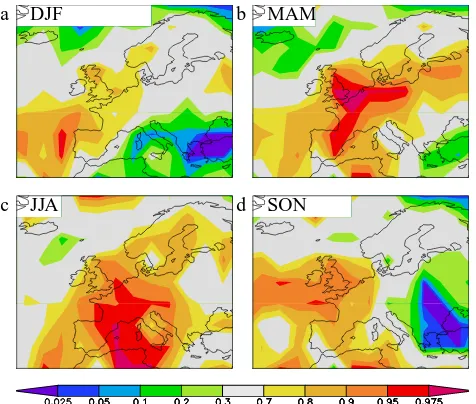
a DJF b MAM

c JJA d SON

Fig. 2. Observed trends in surface temperature (colour, [K/K])

March 1950–February 2008, in the merged HadSST2/CRUTEM3 dataset. (a) December–February, (b) March–May, (c) June–August,

(d) Sep-Nov. A value of one denotes a trend equal to global mean

warming. The contours indicate thez=2, 3 and 4 lines of the signifi-cance of the difference with the modelled trends (ESSENCE ensem-ble). Black (red) indicates that the observed trend is significantly larger (smaller) than the modelled trend.

CRUTEM3+HADSST2

ECHAM5-MPI-OM

GFDL CM2.1

MIROC 3.2 T106

HadGEM1

CCCMA CGCM 3.1 T63

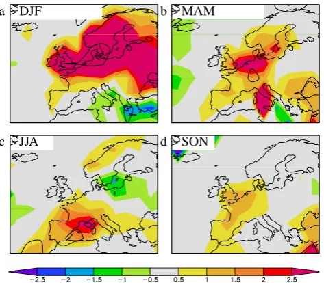
annual mean Dec-Feb Mar-May Jun-Aug Sep-Nov

Fig. 3. The trends in temperature in western Europe as the regression against global mean temperature [K/K] in the observations and the

GCMs with the most realistic mean circulation in Europe over 1950–2007. The contours denote the number of standard errors between the observed and modelled trends starting atz=2 (black) andz=−2 (red).

In all seasons the eastern Atlantic Ocean has warmed sig-nificantly faster than the model simulated. In spring there are also discrepancies of up to 3 standard deviations over land from France to the Baltic and Russia. In summer, the largest discrepancies are in the Mediterranean area, thez=2 contour extending north to the Netherlands. In autumn, over land only Great Britain has 95% significant discrepancies be-tween observed and modelled trends.

The area inside thez=2 contour, 12% to 29% of the area enclosed in 32◦–72◦N, 25◦W–35◦E, is much larger than the 6% expected by chance at 95% confidence. For thez = 3 contour the area is 2% to 6%, larger than the 2.5% expected except in winter. The area expected by chance includes the effects of spatial correlations, assuming 30 degrees of free-dom (Livezey and Chen, 1983).

We performed similar analyses for four other models used for the IPCC Fourth Assessment Report (IPCC, 2007) that simulate the current climate in Europe well (van Ulden and van Oldenborgh, 2006). In Fig. 3 the local temperature trends

over 1950–2007 are shown over Europe in the observations, the ESSENCE ensemble of ECHAM5/MPI-OM model runs, GFDL CM2.1, MIROC 3.2 T106, HadGEM1 and CCCMA CGCM 3.2 T63 models. For the models, we define the trend as the regression against the modelled global mean tempera-ture1. Over western Europe, the patterns of change are sim-ilar to the ones in Fig. 2, although the statistical significance is lower due to the smaller ensemble sizes.

Considering the full CMIP3 ensemble, Fig. 4 shows for each 5◦×5◦grid box the quantile of the observed trend in the distribution defined by the 22-model CMIP3 ensemble, i.e., the fraction of the model ensemble that shows a lower trend than the observed one. As in Fig. 1c, multiple runs of the same model have been weighed by 1/Nrun, so that natural variability is preserved and all models are weighed equally. In many grid boxes at most one ensemble member of one

1_{The MIROC 3.2 T106, HadGEM1 and CCCMA CGCM 3.2}

T63 experiments in the CMIP3 archive exhibit an O(1.5) times

a DJF b MAM

c JJA d SON

Fig. 4. The quantileqof the observed trend in the CMIP3 ensem-ble,q = (N+1/2)/(1+Nmod)withN the number of models in

theNmod=22 model ensemble that have a trend lower than the

ob-served one. If there areNrun>1 runs for one model each run

con-tributes 1/Nrun toN, so that the models are given equal weight.

Purple (q>0.975) indicates that the observed trend is higher than all runs of all models simulate, in the red areas (0.95<q<0.975) one run of one model has a higher trend.

model shows a higher trend than observed. The area corre-sponds geographically to the areas of largez-values in Fig. 2. The highest trend is almost everywhere obtained by run 1 of the three MIROC CGCM3.1 medres experiments, which shows strong warming throughout the Northern Hemisphere. A 17-member perturbed physics ensemble (Murphy et al., 2007) with observed forcing up to 2000 and SRES A1b after-wards exhibits similar behaviour, see Fig. 5. Time slice ex-periments of the PRUDENCE ensemble of high-resolution regional climate models show temperature changes that are similar to the equivalent GCM changes (Christensen and Christensen, 2007).

Over large parts of Europe the observed annual mean tem-perature trends are also outside the range simulated by the re-gional climate models in the ENSEMBLES project that were available, both the 15 models with ERA-40 re-analyis bound-aries and the 11 models with GCM boundbound-aries (not shown).

Figures 2–5 show that the probability is very low that the discrepancy between observed and modelled warming trends is entirely due to natural variability: the area enclosed by the contours is much larger than expected by chance. We there-fore investigate which physical trends are misrepresented in the GCMs.

a DJF b MAM

c JJA d SON

Fig. 5. As Fig. 4, but for a 17-member UK Met ffice perturbed

physics ensemble. Due to the lower number of ensemble members, in this figure red indicates that the observed trend is higher than simulated by any of the ensemble members.

5 Atmospheric circulation

In Europe, at the edge of a continent, changes in tempera-ture are caused to a large extent by changes in atmospheric circulation (Osborn and Jones, 2000; Turnpenny et al., 2002; van Oldenborgh and van Ulden, 2003). To investigate the ef-fects of trends in the atmospheric circulation, monthly mean temperature anomalies are approximated by a simple model that isolates the linear effect of circulation anomalies (van Ulden and van Oldenborgh, 2006; van Ulden et al., 2007). These are the effects of the mean geostrophic wind anoma-liesU0(t ), V0(t )across the temperature gradients, and vor-ticity anomaliesW0(t )that influence cloud cover. The other terms are the direct effect of global warming, approximated again by a linear dependence on the global mean tempera-tureT_global0 (t ), and the remaining noiseη(t ). A memory term Mdescribes the dependence on the temperature one month earlier, which is important near coasts (van Ulden and van Oldenborgh, 2006):

a DJF b MAM

c JJA d SON

Fig. 6. As Fig. 2, but for the circulation-dependent temperature Tcirc.

both in the observations and the models (with coefficients fitted from model data). Temperature changes that are due to changes in the atmospheric circulation show up as trends in T_circ0 . Figure 6 shows the warming trends in the circulation-dependent temperature in the observations and the signifi-cance of the difference with the ECHAM5/MPI-OM climate model results.

In winter, the observed temperature rise around 52◦_{N is}

dominated by circulation changes. Figure 7a shows that a significant increase in air pressure over the Mediterranean (Osborn, 2004) (z>3) and a not statistically significant air pressure decrease over Scandinavia (z<2) have brought more mild maritime air into Europe north of the Alps.

In Fig. 7 trends in sea-level pressure over 1950–2007 of the NCEP/NCAR reanalysis are compared to climate model simulations. Both the reanalysis and the ESSENCE ensem-ble show a significant trend in the Mediterranean region, but the observed trend is a factor four larger than the modelled trend. The GFDL CM2.1 and MIROC 3.2 T106 models also show significant positive trends in this area, but again much smaller than observed. The other two models show no posi-tive trends there.

We conclude that the temperature trends in winter and to a lesser extend spring are due to a shift towards a more west-erly circulation. This change is underrepresented in climate models. In summer and autumn the rise in temperature is mainly caused by factors not linearly related to shifts in at-mospheric circulation.

a b

c d

e f

Fig. 7. Trends in December–February sea-level pressure [hPa/K] over 1950–2007 in the NCEP/NCAR reanalysis (a), ECHAM5/MPI-OM (b), GFDL CM 2.1 (c), MIROC 3.2 T106 (d), CCCMA CGCM 3.1 T63 (e) and HadGEM1 (f).

The contours denote thez-value of the trend being different from zero, starting at 2.

6 Oceanic circulation

The temperature trend in the eastern Atlantic Ocean is un-derestimated by the model results in all seasons but summer and this motivated an investigation of the Atlantic ocean cir-culation. The discrepancy may be either a result of ocean memory of the initial state, or model errors.

-0.6 -0.4 -0.2 0 0.2 0.4 0.6

0 10 20 30 40 50

Essence AMOC Essence AMO HadSST2 AMO

Fig. 8. Autocorrelation function of the ECHAM5/MPI-OM Atlantic

Meridional Overturning Circulation (AMOC) at 35◦N and the

At-lantic Multidecadal Oscillation (AMO) index, SST averaged over 25◦–60◦N, 75◦–7◦W. The effects of external forcing have been minimised by taking anomalies relative to the ensemble mean in the model, and by subtracting the regression against the global mean temperature in the observations.

give weight to temperature variations in the first ten years, when the global mean temperature is almost constant, the ef-fect of ocean memory on the trends is negligible. The fact that the observed trend is outside the ensemble spread there-fore includes the effects of decadal climate variations, to the extent that these are simulated well by the models.

In the observations the multi-decadal oscillations in the Atlantic Ocean are stronger and slower (Fig. 8) than in the ECHAM5/MPI-OM model. Over the last decades there has been a rising trend in the AMO index. To disentangle the effects of the AMO and global warming on temperatures in the North Atlantic region, we subtract a term proportional to the global mean temperature from the SST average, fitted over the 150 years with estimates for both. In the model, this gives the same result as subtracting the ensemble mean (the AMO has very little effect on the global mean temper-ature). Over the relatively short period 1950–2007 we then find virtually no contribution from the AMO on the trend in the observations either.

Systematic model errors play a much larger role. The coarse resolution ocean models used in GCMs have a com-mon error in the North Atlantic Current (NAC). The NAC is compared between the 0.5◦SODA 1.4.1 and 1.4.2 ocean re-analyses (Carton et al., 2005) and the ECHAM5/MPI-OM GCM. Fig. 9c, d show that in the average over the upper 750 m, the warm water of the modelled NAC crosses the basin zonally to Portugal, and continues northward, whereas in the reanalysis this Azores current is much weaker and most water meanders north-east across the Atlantic as part of the surface branch of the Atlantic Meridional Overturning Cir-culation (Lumpkin and Speer, 2003).

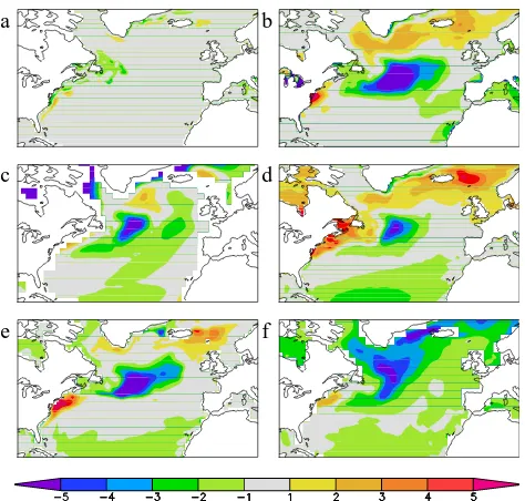
a b

c d

e f

Fig. 9. Ocean surface currents [ms−1] in the SODA reanalysis (a) and the ESSENCE ensemble mean (b), both averaged over 1961– 1990. Northward currents are shown positive, southward currents negative, the colour denotes the total velocity. The same for ver-tically integrated currents from 0 to 750 m [m2s−1] (c, d). Sub-surface temperature [◦C] up to 750 m across the Atlantic Ocean at

53◦N in SODA (e) and the ESSENCE ensemble (f).

The mean vertical thermal structure is shown in Fig. 9e, f at 53◦N. The bias in the currents results in a too weak ver-tical stratification and very deep mixed layers in the mod-elled East Atlantic, where the surface is cooled by cold fresh water advected from the north (due to too strong westerlies that drive a too large southward Ekman drift, Fig. 9a, b) and warmed by the anomalously warm water below (associated with a too far eastward flowing NAC). The deep mixed layer hardly warms under global warming, whereas the observed surface temperature rises at about the same rate as the global mean temperature.

A signature of this bias in the NAC is a strong negative SST bias in the middle of the northern Atlantic Ocean. In the observations this region is south of the NAC, but in the models it is located north of the current and hence it is much colder. Such a bias is clearly visible in all CMIP3 mod-els considered (Fig. 10b–f), but absent when comparing the high-resolution SODA reanalysis to the same lower resolu-tion Oi v2 SST analysis (Fig. 10a) (Reynolds et al., 2002).

a b

c d

e f

Fig. 10. Difference between 1982-2007 annual mean SST and the

OI v2 SST analysis: SODA ocean reanalysis (a), ESSENCE en-semble (b), GFDL CM 2.1 (c), MIROC 3.2 T106 (d), HadGEM1

(e) and CCCMA CGCM 3.1 T63 (f).

with a 5 yr running mean. Trends were removed by taking anomalies with respect to the 17-member ensemble mean. The results are shown in Fig. 11. There is an influence of East Atlantic SST on coastal temperatures of 0.3 to 0.5 K per degree change of East Atlantic SST the previous month, but the signal does not extend very far inland.

7 Soil moisture and short-wave radiation

The third important factor explaining discrepancies between observed and modelled trends in Figs. 2,3 consists of re-lated trends in soil moisture and radiation at the surface in spring and summer. In summer, the pattern of stronger-than-expected heating corresponds closely to the area in which evapotranspiration correlates negatively with temperature in the RCM of Seneviratne et al. (2006) (their Fig. 3a). This indicates that in this area, the soil moisture is exhausted to the extent that an increase in radiation translates directly into a large increase in temperature, whereas in wetter areas the evapotranspiration increases with rising temperature, damp-ing the high temperatures. It should be noted that the ob-served trend (2.6±0.2 over 40◦–50◦N, 0◦–15◦E) is much stronger than the modelled trend (1.4±0.1), indicating that the GCMs underestimate the strength of this process in the current climate.

Regional climate models do not resolve this discrepancy. Comparing the ESSENCE results with the PRUDENCE en-semble (Christensen and Christensen, 2007), we find that the

a b

Fig. 11. Regression of local temperature on SST averaged over

40◦–50◦N, 30◦–10◦W in the ESSENCE ensemble, low-pass fil-tered with a 5yr running mean, sum of monthly 1-month lag regres-sions with SST leading, 1950–2000, anomalies w.r.t. the ensemble mean. December–February (a), June–August (b).

second-highest temperature increases in the Mediterranean, the Alps and southern France between 1960–1990 and 2071– 2100 are no more than 25% higher than the equivalent num-bers for ECHAM5/MPI-OM, whereas the discrepancy be-tween observed and modelled trends approaches a factor two. There is therefore no indication that RCMs simulating the last 50 years would show a warming trend as high as ob-served.

To explain the warming trends further north, we propose a mechanism that closely resembles the mechanism described in Vautard et al. (2007) for extreme summers in Europe. North of the area with most severe drying, southerly winds bring warmer and drier air northwards, increasing the amount of solar radiation reaching the ground. Northerly winds do not change. With the wind direction randomly fluctuating between these two, the net effect is a heating trend accom-panied by soil drying. This way the effects of soil moisture depletion migrate northwards.

We found supporting evidence using Dutch global short-wave radiation observations, which are well-calibrated since the early 1970s (Frantzen and Raaff, 1978). The monthly mean observations were corrected for circulation effects us-ing a model analogous to Eqs. (4)–(6). The trend in circula-tion is small in late spring and summer (cf. Fig. 6), so sub-tracting circulation effects mainly decreases the variability.

a

-5 0 5 10 15 20 25 30 35

ESSENCENetherland

s

De KooyDe BiltEelde VlissingenMaastrichtWagening

en b

-5 0 5 10 15 20 25 30 35

ESSENCENetherland

s

De KooyDe BiltEelde VlissingenMaastrichtWagening

en

Fig. 12. Trends over 1971–2007 in global short-wave radiation

[Wm−2K−1] in spring (a) and summer (b) in the ESSENCE

en-semble of 17 ECHAM5/MPI-OM model experiments, the Nether-lands average, and all stations in the NetherNether-lands. Error bars denote the standard error.

The GCM also has a positive trend in this area, but only 5±2 Wm−2K−1 over 1971–2007. The difference, equiva-lent to a trend of 0.5 in units of global mean temperature, therefore explains half the discrepancy between observations and model in the Netherlands. Spatially, the modelled trend in short-wave radiation is at the northern side of the area of strongest warming in Fig. 2c, in accordance with our hypoth-esis for the summer. In the model the trend is mainly due to a decrease in cloud cover and continues up to 2100, also supporting the hypothesis that the decrease in cloudiness is driven by soil moisture depletion further south. We do not have an explanation for the increased sunshine in spring.

There are indications in the observations that the trend is largest on days with southerly wind directions, both in spring and in summer, but the statistical uncertainty on these results is large. Direct cloud cover observations are unreliable (Nor-ris and Wild, 2007) and uncertainties in cloud cover changes are known to be large (IPCC, 2007), making this mechanism difficult to investigate further using observations, but likely to be relevant.

Land use changes are estimated to contribute O(0.1 K) to the temperature rise in the Netherlands up to now. This value comes from a direct estimate of the effect of grow-ing cities around De Bilt (Brandsma et al., 2003). A rough country-wide estimate can be deduced from the measured in-crease in “built-up area” of 1%/10 yr over 1986–1996 and 1996–2003 (Centraal Bureau voor Statistiek, 2007). Assum-ing that the latent heat flux is halved over this area, this de-creases evaporative cooling by O(2 Wm−2) over 30 years, causing aO(0.1 K)temperature rise. We conclude that land use changes do not contribute substantially to the discrep-ancy between observed and modelled temperature trends.

8 Aerosols

Air pollution has caused a decrease in summer temperatures in Europe from 1950 to around 1985, after this clearer skies (Stern, 2006) have caused a temperature rise (Wild et al., 2005; Norris and Wild, 2007; Wild et al., 2007). This is

re-a

-30 -20 -10 0 10 20 30 40 50

1970 1980 1990 2000 2010 2020 2030 Essence ensemble

De Bilt observations Wageningen observations

b

-30 -20 -10 0 10 20 30 40 50

1970 1980 1990 2000 2010 2020 2030 Essence ensemble

De Bilt observations Wageningen observations

Fig. 13. Modelled global circulation-independent short-wave

radi-ation [Wm−2] compared with observations at the two stations with the longest records in the Netherlands in spring (a) and summer (b).

a b

flected in first a decrease and later an increase in observed short-wave radiation of about 0.3 Wm−2yr−1_{in the} Nether-lands in summer (see Fig. 13). Converting to an annual mean, this is on the low end of the range quoted for the European average of 0.3±0.1 Wm−2yr−1, corrected for cloud cover changes (Norris and Wild, 2007). As the Netherlands, on the coast, escaped the worst affects of air pollution, this dif-ference is not surprising.

The observed decrease over 1970–1985 translates into a cooling effect of 0.3 to 0.4 K. Note that the effect of this tem-porary dimming on the trend over the longer period 1971– 2007 or 1950–2007 is small: the dimming and brightening cancel each other to a large extend.

In our trend measure the effect of decreased solar radiation due to direct and indirect aerosol effects is about 0.2 times the global mean temperature. This explains only a small part of the observed trend in the Netherlands in summer. On shorter time scales, e.g. the period 1985–2007, the reduction of aerosols of course gives a much larger contribution to the temperature trend.

The incoming solar radiation in the ESSENCE ensemble shows a smaller aerosol effect of 0.1±0.1 Wm−2yr−1in the Netherlands in summer. The discrepancy translates into a temperature trend bias of only 0.1±0.1 K per degree global warming, significantly smaller than the effect of the bias in long-term trend discussed above.

9 Snow cover

In spring, differences in modelled and observed snow cover trends amplify the discrepancies in trends in the Baltic re-gion. In Fig. 14 the trend in Mar-May snow cover is shown in the observations and the ESSENCE ensemble. The ob-servations indicate a much faster decrease of spring snow cover than the model. At most grid points the significance of the difference is not very high (p<0.2) because of the large decadal fluctuations in the observed snow cover.

10 Conclusions

We have shown that the discrepancy between the observed temperature rise in western Europe and the trend simulated in present climate models is very unlikely due to fast weather fluctuations or decadal climate fluctuations. The main phys-ical mechanisms are varied, both geographphys-ically and as a function of the seasonal cycle. The most important discrep-ancies between observations and models are

1. a stronger trend to westerly circulation in later winter and early spring in the observations than in the models, 2. a misrepresentation of the North Atlantic Current in the models giving rise to an underestimation of the trend in coastal areas all year,

3. in summer, higher observed than modelled trends in ar-eas in southern Europe where soil moisture depletion is important,

4. a stronger observed trend towards more short-wave ra-diation around the Netherlands in spring and summer than simulated in the climate model.

Smaller contributions come from differences between ob-served and modelled trends in aerosol effects in spring and summer, and snow cover changes in the Baltic in spring.

As most projections of temperature changes in Europe over the next century are based on GCMs and RCMs with the biases discussed above, these projections are probably biased low. To correct the biases, it is essential to not only validate the GCMs for a good representation of the mean climate, but also on the observed temperature trends at regional scales. Acknowledgements. The ESSENCE project, lead by Wilco Hazeleger (KNMI) and Henk Dijkstra (UU/IMAU), was carried out with support of DEISA, HLRS, SARA and NCF (through NCF projects NRG-2006.06, CAVE-06-023 and SG-06-267). We thank the DEISA Consortium (www.deisa.eu), co-funded through EU FP6 projects RI-508830 and RI-031513, for support within the DEISA Extreme Computing Initiative. The authors thank HLRS and SARA staff for technical support.

We acknowledge the other modelling groups for making their sim-ulations available for analysis, the Program for Climate Model Di-agnosis and Intercomparison (PCMDI) for collecting and archiving the CMIP3 model output, and the WCRP’s Working Group on Cou-pled Modelling (WGCM) for organising the model data analysis ac-tivity. The WCRP CMIP3 multi-model dataset is supported by the Office of Science, US Department of Energy.

David Stephenson is thanked for helpful suggestions for the statistical analysis.

Edited by: G. Lohmann

References

Boe, J. and Terray, L.: Uncertainties in summer evapotranspi-ration changes over Europe and implications for regional cli-mate change, Geophys. Res. Lett., 35, L05702, doi:10.1029/ 2007GL032417, 2008.

Brandsma, T., K¨onnen, G. P., and Wessels, H. R. A.: Empirical estimation of the effect of urban heat advection on the temper-ature series of De Bilt (The Netherlands), Int. J. Climatol., 23, 829–845, doi:10.1002/joc.902, 2003.

Brohan, P., Kennedy, J., Haris, I., Tett, S. F. B., and Jones, P. D.: Uncertainty estimates in regional and global observed tempera-ture changes: a new dataset from 1850, J. Geophys. Res., 111, D12106, doi:10.1029/2005JD006548, 2006.

Christensen, J. H. and Christensen, O. B.: A summary of the PRU-DENCE model projectionsof changes in European climate by the end of the century, Clim. Change, 81, 7–30, doi:10.1007/ s10584-006-9210-7, 2007.

Delworth, T. L., Broccoli, A. J., Rosati, A., Stouffer, R. J., Balaji, V., Beesley, J. A., Cooke, W. F., Dixon, K. W., Dunne, J., Dunne, K. A., Durachta, J. W., Findell, K. L., Ginoux, P., Gnanadesikan, A., Gordon, C. T., Griffies, S. M., Gudgel, R., Harrison, M. J., Held, I. M., Hemler, R. S., Horowitz, L. W., Klein, S. A., Knut-son, T. R., Kushner, P. J., Langenhorst, A. R., Lee, H. C., Lin, S. J., Lu, J., Malyshev, S. L., Milly, P. C. D., Ramaswamy, V., Russell, J., Schwarzkopf, M. D., Shevliakova, E., Sirutis, J. J., Spelman, M. J., Stern, W. F., Winton, M., Wittenberg, A. T., Wyman, B., Zeng, F., and Zhang, R.: GFDL’s CM2 global cou-pled climate models – Part 1: Formulation and simulation char-acteristics, J. Climate, 19, 643–674, doi:10.1175/JCLI3629.1, 2006.

Drijfhout, S. S. and Hazeleger, W.: Detecting Atlantic MOC changes in en ensemble of climate change simulations, J. Cli-mate, 20, 1571–1582, doi:10.1175/JCLI4104.1, 2007.

Frantzen, A. J. and Raaff, W. R.: De globale straling in het Rijn-mondgebied (Global Radiation in the greater Rotterdam area), W. R., KNMI, De Bilt, Netherlands, 78–14, 1978.

IPCC: Climate Change 2007: The Physical Science Basis. Contri-bution of Working Group I to the Fourth Assessment Report of the Intergovernmental Panel on Climate Change (IPCC), edited by: Solomon, S., Qin, D., Manning, M., Chen, Z., Marquis, M., Averyt, K. B., Tignor, M., and Miller, H. L., Cambridge Univer-sity Press, Cambridge, UK and New York, NY, USA, 2007. Johns, T., Durman, C., Banks, H., Roberts, M., McLaren, A.,

Ri-dley, J., Senior, C., Williams, K., Jones, A., Keen, A., Rickard, G., Cusack, S., Joshi, M., Ringer, M., Dong, B., Spencer, H., Hill, R., Gregory, J., Pardaens, A., Lowe, J., Bodas-Salcedo, A., Stark, S., and Searl, Y.: HadGEM1 – Model description and anal-ysis of preliminary experiments for the IPCC Fourth Assessment Report, Tech. Rep. 55, UK Met Office, Exeter, UK, 2004. Jungclaus, J. H., Keenlyside, N., Botzet, M., Haak, H., Luo,

J.-J., Latif, M., Marotzke, J., Mikolajewicz, U., and Roeck-ner, E.: Ocean circulation and tropical variability in the cou-pled model ECHAM5/MPI-OM, J. Climate, 19, 3952–3972, doi: 10.1175/JCLI3827.1, 2006.

K-1 model developers: K-1 coupled model (MIROC) description, Tech. Rep. 1, Center for Climate System Research, Univer-sity of Tokyo, www.ccsr.u-tokyo.ac.jp/kyosei/hasumi/MIROC/ tech-repo.pdf, 2004.

Kalnay, E., Kanamitsu, M., Kistler, R., Collins, W., Deaver, D., Gandin, L., Iredell, M., Saha, S., White, G., Woollen, J., Zhu, Y., Leetma, A., Reynolds, R., Chelliah, M., Ebisuzaki, W., Higgens, W., Janowiak, J., Mo, K. C., Ropelewski, C., Wang, J., and Jenne, R.: The NCEP/NCAR 40-year reanalysis project, Bull. Amer. Met. Soc., 77, 437–471, doi:10.1175/1520-0477(1996) 077h0437:TNYRPi2.0.CO;2, 1996.

Kattenberg, A.: De toestand van het klimaat in Nederland 2008, KNMI, www.knmi.nl/toestandklimaat, 2008.

Keenlyside, N. S., Latif, M., Jungclaus, J., Kornblueh, L., and Roeckner, E.: Forecasting North Atlantic Sector Decadal Cli-mate Variability, Nature, 453, 84–88, doi:10.1038/nature06921, 2008.

Kim, S.-J., Flato, G. M., de Boer, G. J., and McFarlane, N. A.: A

coupled climate model simulation of the Last Glacial Maximum, Part 1: transient multi-decadal response, Clim. Dynam., 19, 515– 537, doi:10.1007/s00382-002-0243-y, 2002.

Lenderink, G., van Ulden, A. P., van den Hurk, B., and Keller, F.: A study on combining global and regional climate model results for generating climate scenarios of temperature and precipitation for the Netherlands, Clim. Dynam., 29, 157–176, doi:10.1007/ s00382-007-0227-z, 2007.

Livezey, R. E. and Chen, W. Y.: Statistical Field Significance and its Determination by Monte Carlo Techniques, Mon. Weather Rev.,

111, 46–59, doi:10.1175/1520-0493(1983)111h0046:SFSAIDi2.

0.CO;2, 1983.

Lumpkin, R. and Speer, K.: Large-Scale Vertical and Horizontal Circulation in the North Atlantic Ocean, J. Phys. Oceanogr., 33,

1902–1920, doi:10.1175/1520-0485(2003)033h1902:LVAHCIi

2.0.CO;2, 2003.

Marsland, S. J., Haak, H., Jungclaus, J. H., Latif, M., and R¨oske, F.: The Max-Planck-Institute global ocean/sea ice model with orthogonal curvilinear coordinates, Ocean Modelling, 5, 91–127, doi:10.1016/S1463-5003(02)00015-X, 2003.

Murphy, J. M., Booth, B. B. B., Collins, M., Harris, G. R., Sexton, D., and Webb, M.: A methodology for probabilistic predictions of regional climate change from perturbed physics ensembles, Phil. Trans. R. Soc. A, 365, 1993–2028, doi:10.1098/rsta.2007. 2077, 2007.

Nakicenovic, N. et al.: Special Report on Emissions Scenarios: A Special Report of Working Group III of the Intergovernmental Panel on Climate Change, Cambridge University Press, Cam-bridge, UK, www.grida.no/climate/ipcc/emission/, 2000. Norris, J. R. and Wild, M.: Trends in aerosol radiative effects over

Europe inferred from observed cloud cover, solar “dimming,” and solar “brightening”, J. Geophys. Res., 112, D08214, doi: 10.1029/2006JD00779, 2007.

Osborn, T. J.: Simulating the winter North Atlantic Oscillation: the roles of internal variability and greenhouse gas forcing, Clim. Dyn., 22, 605–623, doi:10.1007/s00382-004-0405-1, 2004. Osborn, T. J. and Jones, P. D.: Air flow influences on local climate:

observed United Kingdom climate variations, Atmos. Sci. Lett., 1, 62–74, doi:10.1006/asle.2000.0017, 2000.

Rahmstorf, S., Cazenave, A., Church, J. A., Hansen, J. E., Keeling, R. F., Parker, D. E., and Somerville, R. C. J.: Recent Climate Observations Compared to Projections, Science, 316, p. 709, doi: 10.1126/science.1136843, 2007.

Rayner, N. A., Brohan, P., Parker, D. E., Folland, C. K., Kennedy, J. J., Vanicek, M., Ansell, T., and Tett, S. F. B.: Improved analy-ses of changes and uncertainties in marine temperature measured in situ since the mid-nineteenth century: the HadSST2 dataset, J. Climate, 19, 446–469, doi:10.1175/JCLI3637.1, 2006.

Reynolds, R. W., Rayner, N. A., Smith, T. M., Stokes, D. C., and Wang, W.: An Improved In Situ and Satellite SST Anal-ysis for Climate, J. Climate, 15, 1609–1625, doi:10.1175/

1520-0442(2002)015h1609:AIISASi2.0.CO;2, 2002.

Scherrer, S. C., Appenzeller, C., Liniger, M. A., and Sch¨ar, C.: European temperature distribution changes in observations and climate change scenarios, Geophys. Res. Lett., 32, L19705, doi: 10.1029/2005GL024108, 2005.

Seneviratne, S. I., L¨uthi, D., Litschi, M., and Sch¨ar, C.: Land-atmosphere coupling and climate change in Europe, Nature, 443, 205–209, doi:10.1038/nature05095, 2006.

Smith, D. M., Cusack, S., Colman, A. W., Folland, C. K., Harris, G. R., and Murphy, J. M.: Improved Surface Temperature Pre-diction for the Coming Decade from a Global Climate Model, Science, 317, 796–799, doi:10.1126/science.1139540, 2007. Sterl, A., Severijns, C., Dijkstra, H., Hazeleger, W., van

Olden-borgh, G. J., van den Broeke, M., Burgers, G., van den Hurk, B., van Leeuwen P. J., and van Velthoven, P.: When can we ex-pect extremely high surface temperatures?, Geophys. Res. Lett., 35, L14703, doi:1029/2008GL034071, 2008.

Stern, D. I.: Reversal of the trend in global anthropogenic sul-fur emissions, Global Env. Change, 16, 207–220, doi:10.1016/ j.gloenvcha.2006.01.001, 2006.

Stott, P. A.: Attribution of regional-scale temperature changes to anthropogenic and natural causes, Geophys. Res. Lett., 30, 1728, doi:10.1029/2003GL01732, 2003.

Turnpenny, J. R., Crossley, J. F., Hulme, M., and Osborn, T. J.: Air flow influences on local climate: comparison of a regional cli-mate model with observations over the United Kingdom, Clicli-mate Res., 20, 189–202, doi:10.3354/cr020189, 2002.

van den Hurk, B. J. J. M., Klein Tank, A. M. G., Lenderink, G., van Ulden, A. P., van Oldenborgh, G. J., Katsman, C. A., van den Brink, H. W., Keller, F., Bessembinder, J. J. F., Burgers, G., Komen, G. J., Hazeleger, W., and Drijfhout, S. S.: KNMI Cli-mate Change Scenarios 2006 for the Netherlands, WR 2006-01, KNMI, www.knmi.nl/climatescenarios, 2006.

van den Hurk, B. J. J. M., Klein Tank, A. M. G., Lenderink, G., van Ulden, A. P., van Oldenborgh, G. J., Katsman, C. A., van den Brink, H. W., Keller, F., Bessembinder, J. J. F., Burgers, G., Komen, G. J., Hazeleger, W., and Drijfhout, S. S.: New Cli-mate Change Scenarios for the Netherlands, Water Sci. Technol., 56, 27–33, doi:10.2166/wst.2007.533, 2007.

van Oldenborgh, G. J. and van Ulden, A. P.: On the relationship between global warming, local warming in the Netherlands and changes in circulation in the 20th century, Int. J. Climatol., 23, 1711–1724, doi:10.1002/joc.966, 2003.

van Ulden, A. P. and van Oldenborgh, G. J.: Large-scale atmo-spheric circulation biases and changes in global climate model simulations and their importance for climate change in Central Europe, Atmos. Chem. Phys., 6, 863–881, 2006,

http://www.atmos-chem-phys.net/6/863/2006/.

van Ulden, A. P., Lenderink, G., van den Hurk, B., and Van Mei-jgaard, E.: Circulation Statistics and Climate Change in Cen-tral Europe: PRUDENCE Simulations and Observations, Clim. Change, 81, 179–192, 2007.

Vautard, R., Yiou, P., D’Andrea, F., de Noblet, N., Viovy, N., Cassou, C., Polcher, J., Ciais, P., Kageyama, M., and Fan, Y.: Summertime European heat and drought waves induced by win-tertime Mediterranean rainfall deficit, Geophys. Res. Lett., 34, L07711, doi:10.1029/2006GL028001, 2007.

Wild, M., Gilgen, H., Roesch, A., Ohmura, A., Long, C. N., Dutton, E. G., Forgan, B., Kallis, A., Russak, V., and Tsvetkov, A.: From Dimming to Brightening: Decadal Changes in Solar Radiation at Earth’s Surface, Science, 308, 847–850, doi:10.1126/science. 1103215, 2005.