www.ocean-sci.net/12/403/2016/ doi:10.5194/os-12-403-2016
© Author(s) 2016. CC Attribution 3.0 License.
Wave extreme characterization using self-organizing maps
Francesco Barbariol1, Francesco Marcello Falcieri1, Carlotta Scotton2, Alvise Benetazzo1, Sandro Carniel1, and Mauro Sclavo1
1Institute of Marine Sciences, Italian National Research Council, Venice, Italy 2University of Padua, Padua, Italy
Correspondence to: Francesco Barbariol ([email protected]) Received: 17 July 2015 – Published in Ocean Sci. Discuss.: 25 August 2015
Revised: 12 January 2016 – Accepted: 23 February 2016 – Published: 10 March 2016
Abstract. The self-organizing map (SOM) technique is con-sidered and extended to assess the extremes of a multivariate sea wave climate at a site. The main purpose is to obtain a more complete representation of the sea states, including the most severe states that otherwise would be missed by a SOM. Indeed, it is commonly recognized, and herein confirmed, that a SOM is a good regressor of a sample if the frequency of events is high (e.g., for low/moderate sea states), while a SOM fails if the frequency is low (e.g., for the most severe sea states). Therefore, we have considered a trivariate wave climate (composed by significant wave height, mean wave period and mean wave direction) collected continuously at the Acqua Alta oceanographic tower (northern Adriatic Sea, Italy) during the period 1979–2008. Three different strate-gies derived by SOM have been tested in order to capture the most extreme events. The first contemplates a pre-processing of the input data set aimed at reducing redundancies; the sec-ond, based on the post-processing of SOM outputs, consists in a two-step SOM where the first step is applied to the orig-inal data set, and the second step is applied on the events ex-ceeding a given threshold. A complete graphical representa-tion of the outcomes of a two-step SOM is proposed. Results suggest that the post-processing strategy is more effective than the pre-processing one in order to represent the wave climate extremes. An application of the proposed two-step approach is also provided, showing that a proper represen-tation of the extreme wave climate leads to enhanced quan-tification of, for instance, the alongshore component of the wave energy flux in shallow water. Finally, the third strategy focuses on the peaks of the storms.
1 Introduction
applied by Masina et al. (2015) to the significant wave height and peak water level in the context of coastal flooding.
Recently, the self-organizing map (SOM) technique has been successfully applied to represent the multivariate wave climate around the Iberian Peninsula (Camus et al., 2011a, b) and the South American continent (Reguero et al., 2013). SOM (Kohonen, 2001) is an unsupervised neural network technique that classifies multivariate input data and projects them onto a uni- or bi-dimensional output space, called map. The SOM technique was originally developed in the 1980s, and has been largely applied in various fields, includ-ing oceanography (Liu et al., 2006; Solidoro et al., 2007; Morioka et al., 2010; Camus et al., 2011a; Falcieri et al., 2013). Typical applications of SOM are vector quantization, regression and clustering. SOMs gained credit among other techniques with same applications due to its visualization ca-pabilities that allow one to get multi-dimensional informa-tion from a two-dimensional lattice. The SOM also has the advantages of unsupervised learning; therefore, vector quan-tization is performed autonomously. However, the quanti-zation is strongly driven by the input data density. Indeed, the SOM is principally forced by the most frequent condi-tions, while the most rare (i.e., the extreme events) are of-ten missed. Consequently, it is highly unlike to find extremes properly represented on a SOM.
In the context of ocean waves, drawing upon the works of Camus et al. (2011a, b) and Reguero et al. (2013), the SOM input is generally constituted by a set of wave param-eters measured or simulated at a given location and evolv-ing over the timet, e.g., the triplet composed by significant wave heightHs(t ), mean wave periodTm(t )and mean wave directionθm(t ), even if other variables can be added (exam-ples of five- or six-dimensional inputs can be found in Ca-mus et al., 2011a). Several activities in the wave field could benefit from the SOM outcomes, such as selection of typi-cal deep-water sea states for propagation towards the coast to study the longshore currents regime and coastal erosion, identification of typical sea states for wave energy resource assessment and wave farm optimization. In addition the em-pirical joint and marginal PDFs can be derived from SOMs. As accurately shown in Camus et al. (2011b), besides inter-esting potentials, especially in visualization, some drawbacks in using the SOM for wave analysis have emerged with re-spect to other classification techniques. Indeed, the largestHs are missed by SOMs because such extreme events are both rare (few comparisons in the “competitive” stage of the SOM learning) and distant from the others in the multi-dimensional space of input data (poorly influenced during the “coopera-tive” stage).
Moving from this evidence, the scientific question being asked is how can we employ SOM with its visualization ca-pabilities to improve representation of the extremes of a mul-tivariate wave climate at a location. To answer this question we have followed three different strategies. First, we have pre-preprocessed the SOM input data using the
maximum-dissimilarity algorithm (MDA) in order to reduce the redun-dancies of the frequent low and moderate sea states, as done by Camus et al. (2011a). Indeed, MDA is a technique that reduces the density of inputs by preserving only the most representative (i.e., the most distant from each other in a Eu-clidean sense). Doing so, the most severe sea states are ex-pected to gain weight in the learning process. We have called this strategy MDA-SOM. Then, we have focused on the post-processing of the SOM outputs. In this context, we have ap-plied a two-step SOM approach (herein called TSOM), by firstly running the SOM to get a reliable representation of the low/moderate (i.e., the most frequent) wave climate, and then by running a second SOM on a reduced input sample. This new sample has been obtained by taking from first-step SOM results the events exceeding a prescribed threshold (e.g., 97th percentile ofHs). To present results of two-step SOMs, we have proposed a double-sided map, showing on the left the SOM with the reliable representation of the low/moderate sea states, and on the right the map with the most severe sea states (i.e., the extremes). Then, we have applied a SOM to the peak of the storms individuated by means of a peak-over-threshold analysis (calling this strategy POT-SOM) and we have represented results using the double-sided map. An ap-plication of the proposed TSOM approach is finally reported: we have exploited the TSOM results to compute the long-shore component of the wave energy flux, showing that a more proper representation of the extreme wave climate leads to an enhanced quantification of the energy approaching the shore.
2 Data
The data set employed for the SOM analysis consists of wave time series gathered at the Acqua Alta oceanographic tower, owned and operated by the Italian National Research Council – Institute of Marine Sciences (CNR-ISMAR). Acqua Alta is located in the northern Adriatic Sea (Italy, northern Mediter-ranean Sea), approximately 15 km off the Venice coast at 17 m depth (Fig. 1) and is a preferential site for marine obser-vations (wind, wave, tide, physical and biogeochemical water properties are routinely retrieved), with a multi-parameter-measuring structure on board (Cavaleri, 2000) upgraded over the years. For this study, we have relied on a 30-year (1979– 2008) data set of 3-hourly significant wave heightHs, mean wave periodTmand mean wave direction of propagationθm (measured clockwise from the geographical north), observed using pressure transducers. Preliminarily, data have been pre-processed in order to remove occasional spikes. To this end, at first the time series have been treated with an ad hoc de-spiking algorithm (Goring and Nikora, 2002). The complete data set is therefore constituted of three variables and 50 503 sea states.
occa-Figure 1. Acqua Alta (AA) oceanographic tower location in the northern Adriatic Sea, Italy (left panel). The tower is depicted in the right panel.
Table 1. Wave climate at Acqua Alta in the period 1979–2008. Mean (h−i), standard deviation (SD), minimum (min),nth percentile (nth perc), and maximum (max) of wave parameters.
h−i SD min 50th perc 95th perc 97th perc 99th perc max
Hs(m) 0.62 0.57 0.05 0.44 1.80 2.12 2.68 5.23
Tm(s) 4.1 1.1 0.5 3.9 6.0 6.35 7.18 10.1
θm(◦N) 260 72 1 270 336 343 353 360
sionally they can reach severe levels: the most intense event (Hs=5.23 m,Tm=5.36 s,θm=242◦N) occurred on 9 De-cember 1992 during a storm forced by winds coming from north-east. Such severe events are not frequent, as confirmed by the 99th percentile ofHs, which is 2.68 m. Nevertheless they populate the wave time series at Acqua Alta and con-stitute the most interesting part of the sample, for instance for extreme analysis. Mean wave period is on average 4.1 s, while mean wave direction is 260◦N indeed most of the waves propagate towards the western quadrants.
This is represented more in detail by the histogram repre-senting the PDF of θm (Fig. 2, bottom panel), which shows that the most frequent directions of propagation are indeed in the range 180 <θm< 360◦N (western quadrants), with peaks at 247.5 and 315◦N. Directions associated with the most in-tense sea states (Hs>4.5 m) can be obtained from the bivari-ate histogram (Hs−θm) representing the joint PDF ofHsand θm(Fig. 2, top panel): 247.5, 270 and 315◦N. Mild sea states and calms (Hs<1.5hHsi, following Boccotti, 2000) are the most frequent conditions at Acqua Alta, with 80 % of occur-rence during the 30 years of observations. They mainly prop-agate towards the western quadrants too, though the princi-pal propagation directions of such seas states is north-west. In this context, the most frequent sea states at Acqua Alta are represented by {Hs, θm} ={0.25 m, 315◦N}. Storms in the area (denoted as sea states withHs≥1.5hHsi) are gen-erated by the dominant winds, i.e., the so-called Bora and Sirocco winds (Signell et al., 2005; Benetazzo et al., 2012). Bora is a gusty katabatic and fetch-limited wind that blows from north-east; it generates intense storms along the
Ital-5% 10%
15% 20%
25%
270◦ 90◦
180◦ 0◦
0–0.5 0.5–1 1–1.5 1.5–2 2–2.5 2.5–3 3–3.5 3.5–4 4–4.5 4.5–5.5 Hs( m)
0 45 90 135 180 225 270 315 360
10−4 10−3 10−2 10−1
p
(
θm
)
θm(◦N) N
Figure 2. Observed bivariate wave climate at Acqua Alta: his-tograms representing the joint PDF ofHsandθm(top panel) and the marginal PDF ofθm(bottom panel). Resolutions are1Hs=0.5 m and1θm=22.5◦.
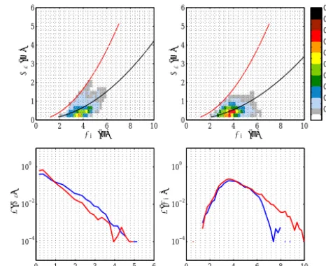
occurrence of 12 % and Sirocco storms an occurrence of 8 %. The most frequent {Hs, Tm}, which occurred in the Bora and Sirocco quadrants, are shown in the bivariate (Hs−Tm) his-togram (Fig. 3) are {0.15 m, 3.6 s} and {0.35 m, 3.8 s}, re-spectively, Sirocco being the most frequent among the two. The associated marginal histogram (Fig. 3) point out that Sirocco winds are responsible for most of the calms, in par-ticular for sea states withHs<1 m, while Bora for the most energetic sea states. Nevertheless, the histogram ofHsshows that Sirocco events with Hs in the range of 4–5 m can oc-cur as well as Bora events. Bora is also associated with the shortest period waves observed: indeed, the histograms ofTm almost coincide for waves shorter than 5.5 s, while for longer waves the probability level of Bora mean periods abruptly drops to values much smaller than those of Sirocco (which remains to non-negligible levels until 9 s). The consequence of shorter and higher Bora waves, with respect to Sirocco, is steeper waves (3 % against 2 % on average, respectively).
3 Self-organizing maps 3.1 Theoretical background
In this section, we recall SOM features that are functional to the study. For more comprehensive readings we refer to Kohonen (2001) and other references cited in the following.
The SOM is an unsupervised neural network technique that classifies multivariate input data and projects them onto a uni- or bi-dimensional output space, called map. Typically a bi-dimensional lattice is produced as output map. The global structure of the lattice is defined by the map shape that can be sheet, cylindrical or toroidal. The local structure of the lattice is defined by the shape of the elements, called units, that are typically either rectangular or hexagonal. The out-put map produced by a SOM on wave inout-put data (e.g., as in Camus et al., 2011a) furnishes an immediate picture of the multivariate wave climate and allows one to identify, among others, the most frequent sea states along with their signif-icant wave height, mean direction of propagation and mean period.
The core of SOM is represented by the learning stage. Therefore, the choice of functions and parameters that con-trol learning is crucial to obtain reliable maps. In SOM, the classification of input data is performed by means of competitive–cooperative learning: at each iteration, the ele-ments of the output units compete among themselves to be the winning or best-matching units (BMUs), i.e., the closest to the input data according to a prescribed metric (compet-itive stage), and they organize themselves due to lateral in-hibition connections (cooperative stage). Usually, given that the chosen metric is a Euclidean distance, inputs have to be normalized before learning (e.g., by imposing unit variance or[0,1]range for all the input variables) and de-normalized once finished. The lateral inhibition among the map units is based upon the map topology and upon a neighboring
func-Tm( s ) Hs
(m
)
0 2 4 6 8 10
0 1 2 3 4 5 6
0 1 2 3 4 5 6
10−4 10−2 100
p
(
H
s
)
Hs( m) 0 2 4 6 8 10
10−4 10−2 100
p
(
Tm
)
Tm(s) Tm( s ) Hs
(m
)
0 2 4 6 8 10
0 1 2 3 4 5 6
p
(
H
s
,T
m
)
0.05 0.1 0.15 0.2 0.25 0.3 0.35 0.4 0.45 0.5
Figure 3. Observed bivariate wave climate at Acqua Alta: his-tograms representing the joint PDFs ofHs andTmfor Bora (top-left panel) and Sirocco (top-right panel) sea states and the corre-sponding marginal PDFs ofHs(bottom-left panel; blue for Bora, red for Sirocco) andTm(bottom-right panels; blue for Bora, red for Sirocco). Black solid lines in the top panels denote average wave steepness 2π Hs/g/Tm2(3 % for Bora, 2 % for Sirocco,gbeing grav-itational acceleration), red solid lines denote wave breaking limit (7 %). Resolutions are1Hs=0.2 m and1Tm=0.2 s.
met-rics. The most common ones are the mean quantization error and the topographic error (Kohonen, 2001). The former is the average of the Euclidean distances between each input data and its BMUs, and is a measure of the goodness of the map in representing the input. The latter is the percentage of input data that have first and second best matching units adjacent in the map and is a measure of the topological preservation of the map.
3.2 SOM setup
In this paper, the SOM technique has been applied by means of the SOM toolbox for MATLAB (Vesanto et al., 2000) that allows for most of the standard SOM capabilities, includ-ing pre- and post-processinclud-ing tools. Among the techniques available, we have chosen the batch algorithm because to-gether with a linear initialization it permits repeatable analy-ses; i.e., several SOM runs with the same parameters produce the same result (Kohonen et al., 2009). This is not a general feature of SOM, as the non-univoque character of both ran-dom initialization and selection of the data in the sequential algorithm lead to always different, though consistent, SOMs (Kohonen, 2001).
Parameters controlling the SOM topology and batch-learning have been accurately examined and their values have been chosen as the result of a sensitivity analysis aimed at attaining the lowest mean quantization and topographic errors. Therefore, we have chosen bi-dimensional squared SOM outputs that are sheet shaped and with hexagonal cells. This kind of topology has been preferred to others (e.g., rect-angular lattice, toroidal shape, rectrect-angular cells) because the maps produced this way had the best topological preservation (low topographic error) and visual appearance. The map’s size is 13×13 (169 cells); hence, each cell represents ap-proximately 300 sea states on average, if the complete data set is considered. The lateral inhibition among the map units is provided by a cut-Gaussian neighborhood function that ensures a certain stiffness to the map (Kohonen, 2001) dur-ing the batch learndur-ing process (1000 iterations). At the same time, to allow the map to widely span the data set, the neigh-borhood radius has been set to 7 at the beginning, i.e., more than half the size of the map, and then it linearly decreased to 1 during a single phase learning process.
Input data have been normalized so that the minimum and maximum distance between two realizations of a variable are 0 and 1, respectively. To this end, according to Camus et al. (2011a), the following normalizations have been used:
H= Hs−min(Hs)
max(Hs)−min(Hs) ,
T = Tm−min(Tm)
max(Tm)−min(Tm) ,
θ=θm/180. (1)
Therefore,H andT range in[0,1], whileθranges in[0,2]. To take into account the circular character ofθmin distance
Figure 4. Single-step SOM output map.Hs: inner hexagons’ color,
Tm: vectors’ length, θm: vectors’ direction, F: outer hexagons’ color. Mean quantization error: 0.06; topographic error: 22 %.
evaluation, following Camus et al. (2011a) we have consid-ered the Euclidean-circular distance as the metric for SOM learning. In this context, the distancedij between input data {Hi, Ti, θi}and SOM unit{Hj, Tj, θj}is defined as
dij= n
Hi−Hj
2
+ Ti−Tj
2
+min |θi−θj|, 2− |θi−θj|
2o
. (2)
The Euclidean-circular distance has been therefore imple-mented in the scripts of SOM toolbox for MATLAB where distance is calculated.
4 SOM strategies to characterize wave extremes In this section, results of the standard SOM approach (ap-plied one time, hence called single-step SOM) and results of the different strategies proposed to improve extremes repre-sentation are presented. The performances of a single-step SOM, MDA-SOM and TSOM are assessed by comparing the wave parameters time series and their empirical marginal PDFs to the time series reconstructed from the results of the different strategies and relative PDFs, respectively. POT-SOM is treated separately because a direct comparison with the other strategies using the described methods is not possi-ble.
4.1 Single-step SOM
SOM’s output. Gradual and continuous change in wave pa-rameters over the cells points out that the topological preser-vation is quite good, as confirmed by the 22 % topographic error.
According to the map, the most frequent sea states are represented by the triplet {0.17 m, 3.5 s, 323◦N}, which substantially resembles the information that one could have gather from the bivariate (Hs−Tm) and (Hs−θm) histograms (Fig. 3), though these are not formally related to one an-other. Most cells show wave propagation directions point-ing towards the western quadrants, as also displayed in the joint and marginal histograms of θm (Fig. 2). The cells de-noting sea states forced by land winds (pointing toward east) are clustered in the top-left corner of the map and have low frequencies of occurrence (individual and cumulated). The frequency of occurrence of calms is 80 %, while that of Bora storms is 12 % and that of Sirocco storms is 8 % (us-ing definition of calms, Bora and Sirocco storm events given in Sect. 2). Hence, the integral distribution of the observed events overHs andθmis retained by SOMs. Sea states with the longest wave periods are clustered in the top-right corner of the map.
The most severe sea states of the map are clustered in the top-right part of the map, but are limited toHsvalues smaller than 2.75 m. Indeed, the triplet with the highestHsproduced by the SOM is {2.75 m, 5.9 s, 270◦N}. However, Tables and histograms in Sect. 2 have shown thatHscan exceed 5.0 m at Acqua Alta. Therefore, sea states withHs>2.75 m are repre-sented by cells with lowerHs. This is clear in Fig. 5, where a sequence of observed events, including one withHs>4.0 m, has been compared to the sequence reconstructed after SOM; i.e., for each sea state of the sequence the triplet assumes the values of the corresponding BMUs. In Fig. 5 sea states with
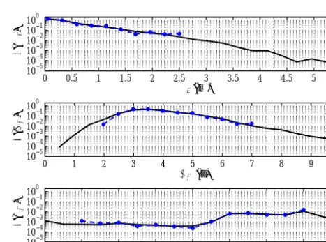
Hs>2.75 m are represented by the cell with the highestHs, i.e., cell no. 118 (first row, 10th column, assuming the cells numbering starts at the top-left cell and proceeds from top to bottom over map rows and then from left to right over map columns); hence,Hsis limited to 2.75 m, whereas the peak of the most severe storm in Fig. 5 has {4.46 m, 6.7 s, 275◦N}. Quantitatively, for this particular event, single-step SOM un-derestimates the peak of 32 %Hs, 12 %Tmand 2 %θm. Al-thoughHsappears to be the most affected (Tmandθmafter a SOM are in better agreement with the original data), all the variables processed by SOM experience a tightening of the original ranges of variation as it is shown in Fig. 6 displaying the marginal empirical PDFs ofHs,Tmandθm after SOM. Generally, PDFs provided by SOMs are in good agreement with the original ones. However, the range of variation ofHs is reduced from [0.05,5.23] to[0.17,2.75]m, the range of
Tmfrom[0.5,10.1]to[2.4,7.4]s, and the range ofθmfrom
[0,360] to[41,323]◦N. The maximumHs value given by SOM (2.75 m) is pretty close to the 99th percentile value (2.68 m), pointing out that SOM provides a good represen-tation of the wave climate up to the 99th percentile approxi-mately. Nevertheless, the remaining 1 % of events not
prop-50 100 150
No. cell
0 5
H
s
(m
)
0 5 10
Tm
(s
)
3310 333 335 337 339 341 343 345 347 349
200
Da y of y e a r 1983 θm
(
◦N
)
Figure 5. Single-step SOM: BMU cells (top panel) and comparison between original (blue solid lines) and reconstructed (red dashed lines) time series of Hs (central-top panel), Tm (central-bottom panel) andθm(bottom panel), for a chosen sequence of events.
0 0.5 1 1.5 2 2.5 3 3.5 4 4.5 5 5.5
10−5
10−4
10−3
10−2
10−1
100
Hs( m)
p
(
H
s
)
0 1 2 3 4 5 6 7 8 9 10
10−5
10−4
10−3
10−2
10−1
100
Tm( s )
p
(
Tm
)
0 45 90 135 180 225 270 315 360
10−5
10−4
10−3
10−2
10−1
100
θm(◦N)
p
(
θm
)
Figure 6. Single-step SOM: comparison of original (black solid line) and resulting (blue dashed dots histograms representing the PDFs ofHs(top panel),Tm(central panel) andθm(bottom panel), for the whole data set.
erly described (extending up to 5.23 m) is for some applica-tions the most interesting part of the sample. This confirms that a single-step SOM provides an incomplete representa-tion of the wave climate.
4.2 Maximum-dissimilarity algorithm and SOM (MDA-SOM)
Table 2. MDA-SOM: absolute errors of average and 99th percentile ofHsafter MDA-SOM relative to the original data set (%).
Hs 100 % 90 % 80 % 70 % 60 % 50 % 40 % 30 % 20 % 10 %
Average 2 4 7 13 15 22 25 32 45 57
99th percentile 9 8 4 5 3 3 5 5 18 27
SOM is constituted by sampling the original data in a way that the chosen sea states have the maximum dissimilarity (herein assumed as the Euclidean-circular distance) one from each other. As a result of MDA, a reduction of the number of sea states with low/moderate Hs, i.e., the most frequent at Acqua Alta, is observed. Hence, MDA-SOM is expected to provide a better description of the extreme sea states. Never-theless, as pointed out by Camus et al. (2011a) the reduction of the sample numerosity leads to lower errors in the 99th percentile ofHs (chosen to represent extremes) but also to higher errors in the average ofHs. Therefore, in terms of per-centage reduction of the original input data set, an optimum balance has to be found in order to get good descriptions of the average and of the extreme wave climate.
In the MDA-SOM application, we have pre-processed the input data set by applying MDA, as described in detail in Camus et al. (2011a). Looking for the best reduction co-efficient, the original data set has been reduced by means of MDA from the initial 50 503 sea states (100 %) to 5050 (10 %), with step 10 %. The absolute errors onhHsiand on the 99th percentile of Hs after MDA-SOM, relative to the original data set, are summarized in Table 2. The error on
hHsi, initially 2 %, monotonically increases up to 57 %, while the error on the 99th percentile ofHs, initially 9 %, decreases down to 3 % at 50–60 % and then increase up to 27 %. With the widening of the variables’ range as principal target (hence a better description of extremes) but without losing the qual-ity on the average climate description, we chose to consider 80 % reduction (7 % error on hHsi, 4 % error on 99th per-centileHs). The corresponding MDA-SOM output displayed in Fig. 7 is topologically equivalent to that produced by the single-step SOM (Fig. 4), except for minor differences on the location of some sea states. However, the most frequent sea state has {Hs,Tm,θm} = {0.28 m, 2.8 s, 328◦N}, which still resembles what has emerged from histograms of Sect. 2, even if Tm is less in agreement with respect to the single-step SOM. Also, the sea state with highestHshas the triplet equal to {2.8 m, 6.0 s, 275◦N}; hence, even if the input data set has been reduced, the representation of extremes is still unsatisfactory.
This is confirmed by the comparison of the original and the reconstructed (after MDA-SOM) time series. In Fig. 8, the comparison has been extended to the results of 60 % MDA-SOM (smaller error on 99th percentileHs, see Table 2) and 10 % MDA-SOM (maximum input data set reduction), in order to investigate if MDA-SOM can enhance extreme wave climate representation even accepting a worsening of
Figure 7. MDA-SOM output map, 80 % reduction of the original data set.Hs: inner hexagons’ color,Tm: vectors’ length,θm: vec-tors’ direction,F: outer hexagons’ color. Mean quantization error: 0.06; topographic error: 15 %.
0 2 4
H
s
(m
)
0 5 10
Tm
(s
)
3310 333 335 337 339 341 343 345 347 349
100 200 300
Day of ye ar 1983
θm
(
◦N
)
Figure 8. MDA-SOM: comparison between original (black solid lines) and reconstructed time series ofHs(top panel),Tm(central panel) andθm(bottom panel), for a chosen sequence of events. Data set reduction: 80 % (blue dashed line), 60 % (red dashed line) and 10 % (green dashed line).
provided by 10 % MDA-SOM, though the maximum is how-ever missed and in its proximity the original data are timated. Indeed, 60 % and 10 % MDA-SOMs locally overes-timateHsin the low/moderate sea states.
The marginal empirical PDFs after MDA-SOM are com-pared in Fig. 9 to the PDFs of the original data set. The distri-butions are in good agreement and the representation is more complete with respect to the single-step SOM, especially concerning Hs. Nevertheless, 10 % MDA-SOM distribution forHsexhibits a larger departure from the original distribu-tion at 1.7 m with respect to the single-step SOM. Also 10 % MDA-SOM distributions, which provides the widest ranges, locally depart from the reference distributions, in particular forTmandθm. The frequency of occurrence of calms is 81 %, while that of Bora storms is 12 % and that of Sirocco storms is 7 %. Hence, except for a minor change in the frequency of calms and Sirocco events, the overall statistics resembles that one directly derived from the Acqua Alta data set.
4.3 Two-step SOM (TSOM)
A TSOM has been then applied to provide a more complete description of the wave climate at Acqua Alta. To this end, the SOM algorithm has been run a first time on the original data set, without reductions (first step). Then, outputs have been post-processed: a thresholdHs∗has been fixed, and the cells having Hs>Hs∗ have been considered to constitute a new input data set that is composed of the sea states repre-sented by the cells exceeding the threshold. Hence, a second SOM has been run on the new data set (second step). Using the same SOM setup as in the first step, we have obtained a two-sided map (Fig. 10): the first map (left panel) provides a good representation of the low/moderate wave climate but fails in the description of the most severe sea states, which are described in the second map (right panel), focusing on the climate overHs∗. Three thresholds have been tested that correspond to the 95th, 97th and 99th percentile ofHs: 1.80, 2.12 and 2.68 m, respectively. In the following, we have fo-cused on the results with 97th percentile threshold, since they have turned out to be more representative of the extreme wave climate than the others.
Figure 10 depicts TSOM results withHs∗=2.12 m (97th percentile). The first map, on the left, is the map shown in Fig. 4, representing the whole wave climate at Acqua Alta. On that map, the six cells with Hs>2.12 m have been en-compassed by a black line. Without such cells, the map on the left represents the low/moderate sea states, i.e., the 97 % of the whole original data set constituted by events withHs below or equal to the 2.12 m threshold. The remaining 3 % of events, represented by the encompassed cells, are the most severe events at Acqua Alta. The first step SOM associates to such events 2.12≤Hs≤2.75 m, 5.0≤Tm≤6.5 s and 249≤θm≤299◦N. Hence, according to SOMs, the most severe sea states pertain to a rather narrow directional sec-tor (50◦) hardly allowing one to discriminate between Bora
0 0.5 1 1.5 2 2.5 3 3.5 4 4.5 5 5.5
10−5
10−4
10−3
10−2
10−1
100
Hs( m)
p
(
H
s
)
0 1 2 3 4 5 6 7 8 9 10
10−5
10−4
10−3
10−2
10−1
100
Tm( s )
p
(
Tm
)
0 45 90 135 180 225 270 315 360
10−5
10−4
10−3
10−2
10−1
100
θm(◦N)
p
(
θm
)
Figure 9. MDA-SOM: comparison between original (black solid lines) and resulting histograms representing the PDFs ofHs (top panel),Tm(central panel) andθm(bottom panel), for the whole pe-riod of observations. Data set reduction: 80 % (blue dashed-squares line), 60 % (red dashed-circles line) and 10 % (green dashed line).
and Sirocco conditions. A more detailed representation of such extremes is provided by the second map in Fig. 10, on the right, where extreme Bora and Sirocco events are more widely described by cells. Indeed, a sort of diagonal (from the top-right corner to the bottom-left corner of the map) di-vides the cells. Bora events are clustered on the left of this diagonal (top-left part of the map), while Sirocco ones on the right of that (bottom-right part of the map). On the diag-onal, cells represent sea states that travel towards the west. This configuration somehow resembles the one observed in the left map, except for the land sea states, in the top-left corner. The most severe sea states are clustered in the top-right corner of the map and also, though to a smaller ex-tent, in the bottom-left part of it. The resulting ranges of
Hs,Tmandθmare 1.94≤Hs≤4.26 m, 4.4≤Tm≤8.3 s and 224≤θm≤316◦N, respectively.
The widened ranges of wave parameters provided by a TSOM allow for a more complete description of the sea states at Acqua Alta, including the most severe as it is shown in Fig. 11. There, for the sequence of events presented in pre-vious sections, the reconstructed TSOM time series is com-pared to the original one. Also results with 95th and 99th percentile TSOMs are plotted, and it clearly appears that the differences among the three tests (i.e., TSOMs withHs threshold on 95th, 97th and 99th percentiles) are very small, in particular for what concerns θm. Nevertheless, the 95th percentile TSOM yields a smaller estimate of the highest
Hs peak with respect to the others, and the 99th percentile TSOM deviates more than the others from the originalTm.
Such differences are also found in the marginal empiri-cal PDFs of the wave parameters, shown in Fig. 12. Indeed,
Figure 10. TSOM output map with thresholdHs∗=2.12 m (97th percentile ofHs).Hs: inner hexagons’ color,Tm: vectors’ length,θm: vectors’ direction, F: outer hexagons’ color. Wave climate after a single-step SOM (left panel) and TSOM extreme wave climate (i.e., over the threshold, right panel and cells within black solid line in the left panel). For the right panel map, mean quantization error: 0.04; topographic error: 6 %.
0 2 4
H
s
(m
)
0 5 10
Tm
(s
)
331 333 335 337 339 341 343 345 347 349
0 100 200 300
Day of ye ar 1983
θm
(
◦N
)
Figure 11. TSOM: comparison between original (black solid lines) and reconstructed time series ofHs(top panel),Tm(central panel) and θm(bottom panel), for a chosen sequence of events. Thresh-olds: 95th (blue dashed line), 97th (red dashed line) and 99th (green dashed line) percentile ofHs.
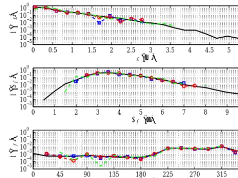
and also from the original PDF, in particular in the largest values ofHsandTm. As expected, the more the threshold is high, the moreHs range widens, extending to higher values. Hence, the 99th percentile TSOM provides the more com-plete representation of the wave climate, at least concerning
Hs. Indeed, the widest Tmrange is obtained with 97th per-centile and the narrowest with a 99th perper-centile TSOM. In-stead, p(θm)is equally represented by the three thresholds and is in excellent agreement with the original PDF, though theθmrange is limited with the respect to the complete circle. In addition, local departure from the original PDFs are still observed, especially forHsandTm. The frequency of occur-rence of calms is 81 %, while that of Bora storms is 11 %
0 0.5 1 1.5 2 2.5 3 3.5 4 4.5 5 5.5
10−5
10−4
10−3
10−2
10−1
100
Hs( m)
p
(
H
s
)
0 1 2 3 4 5 6 7 8 9 10
10−5
10−4
10−3
10−2
10−1
100
Tm( s )
p
(
Tm
)
0 45 90 135 180 225 270 315 360
10−5
10−4
10−3
10−2
10−1
100
θm(◦N)
p
(
θm
)
Figure 12. TSOM: comparison of original (black solid line) and resulting histograms representing the PDFs ofHs (top panel),Tm (central panel) and θm (bottom panel), for the whole data set. Thresholds: 95th (blue squares line), 97th (red dashed-circles line) and 99th (green dashed line) percentile ofHs.
and that of Sirocco storms is 8 %. Hence, except for a minor change in the frequency of calms and Bora events, the overall statistics resembles that one observed at Acqua Alta. 4.4 Peak-over-threshold SOM (POT-SOM)
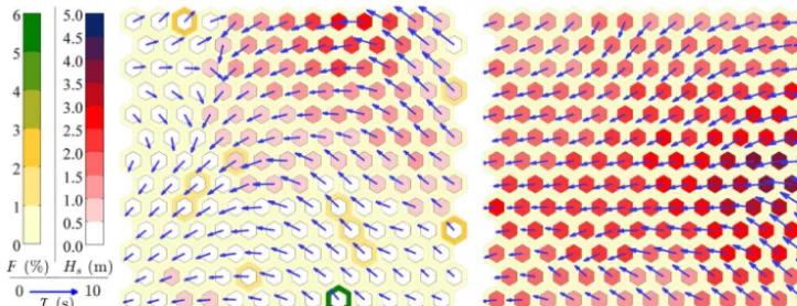
Figure 13. POT-SOM output map.Hs: inner hexagons’ color,Tm: vectors’ length,θm: vectors’ direction,F: outer hexagons’ color. Wave climate after single-step SOM (left panel) and stormy wave climate (right panel). For the right panel map, mean quantization error: 0.06; topographic error: 12 %.
Table 3. Performance summary of different SOM approaches, through the comparisons of reconstructed to original time series, and resulting to original PDFs.rav: ratio of time series averages,rSD: ratio of time series standard deviations, CC: time series cross-correlation coefficient, RMSE: time series root mean square error, CCPDF: PDFs cross-correlation coefficient, RMSEPDF: PDFs root mean square error).
Hs rav rSD CC RMSE (m) range (m) CCPDF RMSEPDF
Single-step SOM 0.98 0.91 0.95 0.18 [0.17,2.75] 1.00 0.04 MDA-SOM (80 %) 1.00 0.90 0.95 0.19 [0.21.2.82] 0.99 0.04 TSOM (97th perc) 0.99 0.95 0.96 0.16 [0.17,4.26] 1.00 0.04
Tm rav rSD CC RMSE (s) range (s) CCPDF RMSEPDF
Single-step SOM 1.00 0.89 0.95 0.34 [2.4,7.4] 0.99 0.02 MDA-SOM (80 %) 1.00 0.90 0.95 0.37 [2.4,7.4] 0.95 0.05 TSOM (97th perc) 1.00 0.90 0.95 0.32 [2.4,8.3] 0.99 0.02
θm rav rSD CC RMSE (◦N) range (◦N) CCPDF RMSEPDF
Single-step SOM 1.00 0.92 0.95 23 [41,323] 0.97 0.00 MDA-SOM (80 %) 0.99 0.95 0.96 20 [30,328] 0.98 0.00 TSOM (97th perc) 1.00 0.92 0.95 23 [41,323] 0.97 0.00
considered thehHsiat Acqua Alta (Table 1) and then, with Hs∗=0.93 m, we individuated 710 storms. The peaks of the storms constitute a new data set that has been analyzed by means of a SOM. At the end, we have obtained a double-sided map that represent at the same time the whole wave climate (on the left) and the “stormy” part of it (on the right). POT-SOM output map is shown in Fig. 13. As expected, stormy events are Bora and Sirocco events: the former are clustered on the upper and middle part of the map, the lat-ter in the lower part of it. The most severe storms, concen-trated on the right side of the map, are both Bora and Sirocco events. The triplet with the highest Hs is {4.27 m, 6.32 s, 265◦N} and the maximum Hs value is very close to the 99th percentile ofHsof the new data set, i.e., 4.28 m. Hence, 99 % of the stormy events are included within the represented range, resembling what was observed for the original data set analyzed with a single-step SOM.
5 Discussion
(below 0.19 m for Hs, 0.37 s forTm and 23◦for θm). Nev-ertheless, the highest ratios and correlation coefficients, and the lowest RMSE pertain to TSOMs. Similar conclusions can be drawn for the PDFs, which are reproduced with very high CC (over 0.95) and RMSEPDF (below 0.04) by all the ap-proaches, but to a greater extent by TSOMs. As expected, the most wide range variability among the different strategies concerns Hs. With the only exception ofθm, whose widest range is provided by MDA-SOM, TSOM turned out to be the most efficient in providing the most complete representation among the tested strategies.
We verified that a higher size single-step SOM (e.g., 25×25, not shown here) can produce a wider range of ex-tremes with respect to that used in the study (i.e., 13×13): the units’ maximum Hs is 3.56 m instead of 2.75 m. In the same map configuration (i.e., 25×25), MDA preselection can further widen this range towards extremes: 3.63 m, the units’ maximumHs obtained with an 80 % reduction of the sample (using MDA); 3.66 m, the units’ maximumHswith a 40 % reduction. This has the effect of reducing the absolute error on 99th percentile ofHs (1 % with 80 % reduction and 11 % with 40 % reduction). However, the most extreme sea states are still far from being properly represented (we recall that the most extreme sea state observed hadHs=5.23 m). In addition and most importantly, if a larger number of ele-ments in the map can improve the SOM performance shown in the paper, it will certainly worsen the readability of the map and the possibility of extracting quantitative information from the map. Indeed, considering, for instance, the 25×25 map, sea states at a site would be represented by 625 typi-cal sea states: a huge number that is hardly manageable for a practical classification of the wave conditions.
6 Application of TSOM
An application of the TSOM is proposed to show that a more detailed representation of the extreme wave climate can en-hance the quantification of the longshore component of the shallow-water wave energy flux P (per unit shore length), expressed as (Komar and Inman, 1970)
P =Ecgsinαcosα, (3)
whereE=ρgHs2/16 is the wave energy per unit crest length (being ρ the water density), cgis the group celerity and α is the mean wave propagation direction measured counter-clockwise from the normal to the shoreline. P is a driving factor for the potential longshore transport, and its depen-dence upon the wave energy E (which in turn depends on the square ofHs) suggests that an accurate representation of Hs is crucial. As the shoreline in front of Acqua Alta tower is almost parallel to the 20◦N direction (i.e., orthogonal to the 290◦N direction), the longshore transport is directed to-wards southwest when P is positive, and directed towards northeast when P is negative. Given the wave energy flux
Ecg,P is maximized whenα= ±45◦N, which correspond toθm=245◦N andθm=335◦N, respectively.
In order to obtain the shallow-water values of wave pa-rameters, following Reguero et al. (2013), we propagated the Acqua Alta sea state resulting from the TSOM (see maps in Fig. 10) from 17 to 5 m depth (a typical closure depth in the region), approximately accounting for the wave trans-formations, i.e., shoaling, refraction and wave breaking. In doing so, we assumed straight and parallel bottom contour lines, we neglected wave energy dissipation prior to wave breaking, and we allowedHs to reach the 80 % of the wa-ter depth at most (depth-induced wave breaking criwa-terion). Roughly, shoaling mostly affects the Sirocco sea states that are typically associated with longer wavelengths with respect to Bora sea states. In shallow water, refraction tends to reduce the difference between Bora and Sirocco directions with re-spect to Acqua Alta, as the normal direction to the shoreline, which waves tend to align to, is very close to the boundary (i.e., 270◦N), which we assumed in order to discriminate be-tween the two conditions. Sea states forced by land winds (20◦N <θm<200◦N) were excluded from the analysis.
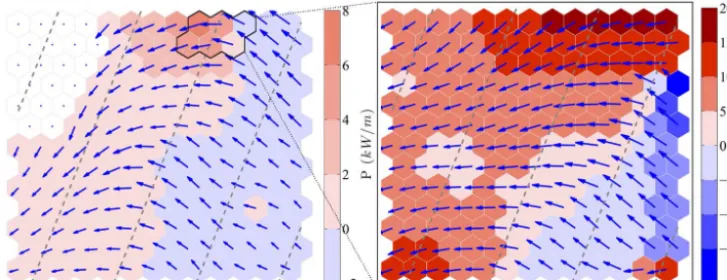
The longshore component of the wave energy fluxP at 5 m depth is shown in Fig. 14. It is worth noting that the left map represents the longshore component of the wave energy flux resulting from the single-step SOM technique (e.g., the left panel of Fig. 10). Here,P ranges between−2 and 8 kW m−1, and the highest values are mainly due to Bora events that are responsible for potential longshore transport towards south-west (even if few Sirocco events withθmclose to 270◦N have the same effect). According to the left map, the transport to-wards northeast is due to Sirocco events that, however, cause less intense potential transport. The highestP values are as-sociated with the highestHsevents, clustered on the cells at the top of the Fig. 10 left map. The right map of Fig. 14 describes the longshore flux component due to the Acqua Alta sea states represented by the SOM cells exceeding the 97th percentileHs threshold (i.e., the six cells bounded by the black line in the left map). The range of P variation widens considerably when the extreme sea states are con-sidered, with values ranging from−20 to 20 kW m−1. As ob-served in the right map of Fig. 10, the sea states exceeding the 97th percentile threshold onHsare Bora and Sirocco events. The Bora events in the top-left part of the map (except for two cells in the bottom-right corner) contribute to positive, i.e., south-westward, transport, while Sirocco events in the bottom-right part contribute to negative, i.e., north-eastward, transport. The most intense transport is associated with the highestHscells at the bottom-left, bottom-right and top-right corners of the Fig. 10 right map. The major difference with respect to a single-step SOM estimate concerns the Sirocco sea states, associated with negativeP, that had the most in-tense value extended from−2 to−20 kW m−1.
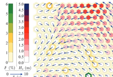
Figure 14. Application of TSOM: assessment of the longshore flux of wave energyPin shallow water, after single-step SOM (left panel) and resulting from the TSOM extreme wave climate (right panel and cells within black solid line in the left panel). Mean wave directions at Acqua Alta tower (blue arrows) indicate contributions of different meteorological conditions: positive mainly due to Bora (180≤θm≤270◦N), negative to Sirocco (270<θm≤360◦N). Land wind events (white cells) have been excluded, and the direction of the shoreline (270◦N) is shown as gray dashed lines.
Table 4. Application of TSOM: assessment of the longshore flux of wave energy in shallow-waterP.Pis the mean over the 1979–2008 period accounting for the absolute value ofP,P+is the mean of the
positiveP, andP−is the mean of the negativeP,1TSOM−SOMis the relative difference of values computed after TSOM with respect to values computed after SOM.
SOM (kW m−1) TSOM (kW m−1) 1TSOM−SOM(%)
P 0.52 0.57 9.0
P+ 0.41 0.45 7.5
P− −0.11 −0.13 16.5
taking the absolute value ofP from the maps of Fig. 14 and is 0.57 kW m−1(Table 4). In order to support this estimate, we compared the 1.71 kW m−1estimate of the mean wave energy fluxEcgat Acqua Alta against the 1.5 kW m−1value obtained at the same site over 1996–2011 by Barbariol et al. (2013). The contributions toP from Bora (P+) and Sirocco
(P−) are 0.45 and−0.12 kW m−1, respectively, pointing out
the predominant effect of Bora on the longshore transport over the western side of the Gulf of Venice. For comparison,
P was also computed using single-step SOM results (see Ta-ble 4): in this case,P is 0.52 kW m−1,P+ is 0.41 kW m−1
andP−is−0.11 kW m−1. Hence, with respect to the TSOM,
the estimate of the mean longshore energy flux is 9.0 % lower forP, 7.5 % lower forP+and 16.5 % lower forP−.
7 Conclusions
In this paper, we have tested different strategies aimed at im-proving the characterization of multivariate wave climate us-ing SOM. Indeed, we have verified that besides a satisfac-tory description of the low/moderate wave climate (in agree-ment with usual uni- and bivariate histograms), the
single-step SOM approach misses the most severe sea states, which are hidden in SOM cells withHseven considerably smaller than the extreme ones.
For our purpose, we used the 1979–2008 trivariate wave climate {Hs,Tm, andθm} recorded at Acqua Alta tower, and we showed that, for instance, the single-step SOM assigned most of the sea states withHs>2.75 m to the {2.75 m, 5.9 s, 270◦N} class. Hence, the most interesting part of the wave
classifi-cation of the storms peaks, based on the peak-over-threshold approach, on the right (POT-SOM).
Finally, a TSOM was applied for the assessment of the potential longshore wave energy flux to show how practical oceanographic and engineering applications can benefit from this novel SOM strategy. Indeed, the mean flux in front of the Venice coast was found to be 9 % higher if evaluated after a TSOM instead of a SOM.
Acknowledgements. The research was supported by the Flagship
Project RITMARE – The Italian Research for the Sea-coordinated by the Italian National Research Council and funded by the Italian Ministry of Education, University and Research within the National Research Program 2011–2015. The authors gratefully acknowledge Luigi “Gigi” Cavaleri for providing wave data at Acqua Alta tower and for the fruitful discussions. The authors wish to thank Renata Archetti (UNIBO, Italy) and three anonymous referees for the useful comments that helped improve the paper.
Edited by: V. Brando
References
Barbariol, F., Benetazzo, A., Carniel, S., and Sclavo, M.: Improving the assessment of wave energy resources by means of coupled wave-ocean numerical modeling, Renew. Energ., 60, 462–471, 2013.
Benetazzo, A., Fedele, F., Carniel, S., Ricchi, A., Bucchignani, E., and Sclavo, M.: Wave climate of the Adriatic Sea: a future sce-nario simulation, Nat. Hazards Earth Syst. Sci., 12, 2065–2076, doi:10.5194/nhess-12-2065-2012, 2012.
Boccotti, P.: Wave mechanics for ocean engineering, vol. 64, Else-vier Science, Amsterdam, the Netherlands, 2000.
Camus, P., Cofiño, A. S., Mendez, F. J., and Medina, R.: Multivariate wave climate using self-organizing maps, J. At-mos. Ocean. Tech., 28, 1554–1568, doi:10.1175/JTECH-D-11-00027.1, 2011a.
Camus, P., Mendez, F. J., Medina, R., and Cofiño, A. S.: Analysis of clustering and selection algorithms for the study of multivariate wave climate, Coast. Eng., 58, 453–462, doi:10.1016/j.coastaleng.2011.02.003, 2011b.
Cavaleri, L.: The oceanographic tower Acqua Alta – activity and prediction of sea states at Venice, Coast. Eng., 39, 29–70, doi:10.1016/S0378-3839(99)00053-8, 2000.
De Michele, C., Salvadori, G., Passoni, G., and Vezzoli, R.: A multi-variate model of sea storms using copulas, Coast. Eng., 54, 734– 751, doi:10.1016/j.coastaleng.2007.05.007, 2007.
Falcieri, F. M., Benetazzo, A., Sclavo, M., Russo, A., and Carniel, S.: Po River plume pattern variability investigated from model data, Cont. Shelf Res., 87, 84–95, doi:10.1016/j.csr.2013.11.001, 2013.
Goring, D. G. and Nikora, V. I.: Despiking Acoustic Doppler Velocimeter Data, 128, 117–126, doi:10.1061/(ASCE)0733-9429(2002)128:1(117), 2002.
Isobe, M.: On joint distribution of wave heights and directions, in: Coastal Engineering Proceedings, 1, 524–538, 1988.
Kohonen, T.: Self-Organizing Maps, Springer Series in Infor-mation Sciences, Springer, Berlin-Heidelberg, Germany, 30, doi:10.1007/978-3-642-56927-2, 2001.
Kohonen, T., Nieminen, I. T., and Timo, H.: On the Quantization Error in SOM vs. VQ: A Critical and Systematic Study, in: Advances in Sel-Organizing Maps, Springer, Berlin-Heidelberg, Germany, p. 374 2009.
Komar, P. and Inman, D.: Longshore sand transport on beaches, J. Geophys. Res., 75, 5914–5927, doi:10.1029/JC075i030p05914, 1970.
Kwon, J. and Deguchi, I.: On the Joint Distribution of Wave Height, Period and Direction of Individual Waves in a Three-Dimensional Random Sea, in: Coastal Engineering Proceedings, 1, 370–383, 1994.
Liu, Y., Weisberg, R. H., and He, R.: Sea surface temperature patterns on the West Florida Shelf using growing hierarchi-cal self-organizing maps, J. Atmos. Ocean. Tech., 23, 325–338, doi:10.1175/JTECH1848.1, 2006.
Longuet-Higgins, M. S.: On the Joint Distribution of Wave Pe-riods and Amplitudes in a Random Wave Field, P. Roy. Soc. Lond. A Mat., 389, 241–258, http://rspa.royalsocietypublishing. org/content/389/1797/241.abstract, 1983.
Masina, M., Lamberti, A., and Archetti, R.: Coastal flooding: A copula based approach for estimating the joint proba-bility of water levels and waves, Coast. Eng., 97, 37–52, doi:10.1016/j.coastaleng.2014.12.010, 2015.
Mathisen, J. and Bitner-Gregersen, E.: Joint distributions for signifi-cant wave height and wave zero-up-crossing period, Appl. Ocean Res., 12, 93–103, doi:10.1016/S0141-1187(05)80033-1, 1990. Morioka, Y., Tozuka, T., and Yamagata, T.: Climate variability in
the southern Indian Ocean as revealed by self-organizing maps, Clim. Dynam., 35, 1059–1072, doi:10.1007/s00382-010-0843-x, 2010.
Ochi, M. K.: On long-term statistics for ocean and coastal waves, in: Coastal Engineering Proceedings, 1, 59–75, 1978.
Reguero, B. G., Méndez, F. J., and Losada, I. J.: Vari-ability of multivariate wave climate in Latin America and the Caribbean, Global Planet. Change, 100, 70–84, doi:10.1016/j.gloplacha.2012.09.005, 2013.
Signell, R. P., Carniel, S., Cavaleri, L., Chiggiato, J., Doyle, J. D., Pullen, J., and Sclavo, M.: Assessment of wind quality for oceanographic modelling in semi-enclosed basins, J. Marine Syst., 53, 217–233, 2005.
Solidoro, C., Bandelj, V., Barbieri, P., Cossarini, G., and Fonda Umani, S.: Understanding dynamic of biogeochemical prop-erties in the northern Adriatic Sea by using self-organizing maps and k-means clustering, J. Geophys. Res., 112, 1–13, doi:10.1029/2006JC003553, 2007.
Vesanto, J., Himberg, J., Alhoniemi, E., and Parhankangas, J.: SOM Toolbox for Matlab 5, Technical Report A57, 2, 59, available at: http://www.cis.hut.fi/somtoolbox/package/papers/ techrep.pdf (last access: 7 March 2016), 2000.