https://doi.org/10.5194/os-14-1127-2018 © Author(s) 2018. This work is distributed under the Creative Commons Attribution 4.0 License.
World Ocean Circulation Experiment – Argo Global
Hydrographic Climatology
Viktor Gouretski
Integrated Climate Data Center, Center for Earth System Research and Sustainability, The University of Hamburg, Grindelberg 5, 20144 Hamburg, Germany
Correspondence:Viktor Gouretski ([email protected]) Received: 13 March 2018 – Discussion started: 6 April 2018
Revised: 21 August 2018 – Accepted: 3 September 2018 – Published: 27 September 2018
Abstract.The paper describes the new gridded World Ocean Circulation Experiment-Argo Global Hydrographic Clima-tology (WAGHC). The climaClima-tology has a 1/4◦spatial reso-lution resolving the annual cycle of temperature and salinity on a monthly basis. Two versions of the climatology were produced and differ with respect to whether the spatial inter-polation was performed on isobaric or isopycnal surfaces, re-spectively. The WAGHC climatology is based on the quality controlled temperature and salinity profiles obtained before January 2016, and the average climatological year is in the range from 2008 to 2012.
To avoid biases due to the significant step-like decrease of the data below 2 km, the profile extrapolation proce-dure is implemented. We compare the WAGHC climatol-ogy to the 1/4◦ resolution isobarically averaged WOA13
climatology, produced by the NOAA Ocean Climate Lab-oratory (Locarnini et al., 2013) and diagnose a generally good agreement between these two gridded products. The differences between the two climatologies are basically at-tributed to the interpolation method and the considerably ex-tended data basis. Specifically, the WAGHC climatology im-proved the representation of the thermohaline structure, in both the data poor polar regions and several data abundant regions like the Baltic Sea, the Caspian sea, the Gulf of Cal-ifornia, the Caribbean Sea, and the Weddell Sea. Further, the dependence of the ocean heat content anomaly (OHCA) time series on the baseline climatology was tested. Since the 1950s, both of the baseline climatologies produce al-most identical OHCA time series. The gridded dataset can be found at https://doi.org/10.1594/WDCC/WAGHC_V1.0 (Gouretski, 2018).
1 Introduction
The description of the mean state of the global ocean has a long history. Since the late 19th century, the continuously growing net of hydrographic observations has resulted in the production of increasingly detailed maps of temperature, salinity, and other parameters. All of these maps were hand drawn, often having the imprint of strong subjective data in-terpretation. The introduction of computers permitted the ac-cumulation and analysis of large amounts of data and led to the construction of the objectively analyzed maps. The first climatology of the world ocean by Levitus (1982) has become a standard for the oceanographic community. Since then the NOAA (National Oceanic and Atmospheric Admin-istration) NCEI (National Centers for Environmental Infor-mation, the former NODC) Ocean Climate Laboratory has regularly produced improved versions of the global climatol-ogy (Levitus et al., 1994, 1998; Locarnini et al., 2006, 2010). The last update (Locarnini et al., 2013) was based on the hy-drographic data over the entire time period from the begin-ning of the hydrographic observations to 2013.
be averaged on isopycnal surfaces. The objective analysis on density surfaces mimics the process of isopycnal mix-ing and does not produce artificial water masses. Gouret-ski and Koltermann (2004) prepared the isopycnally aver-aged Global Hydrographic Climatology (WGHC) based on the high-quality data obtained during the World Ocean Circu-lation Experiment (WOCE). To achieve reasonable data cov-erage between the WOCE section lines, selected pre-WOCE hydrographic data were added to the WOCE dataset, which served as a reference dataset for the calculation of the sys-tematic inter-cruise property offsets (Gouretski and Jancke, 2001). The WGHC was used in a number of applications (e.g., the WOCE Hydrographic Atlas of the Atlantic Ocean – Koltermann et al., 2011; and the calculation of the absolute salinity – IOC, SCOR and IAPSO, 2010). One of the faults of the WGHC climatology is the absence of seasonality: only data mean parameter distributions are available at all levels. More recently a global monthly isopycnal upper-ocean cli-matology with an emphasis on preserving a surface mixed layer was created (Schmidtko et al., 2013).
The purpose of the current study is to produce an update of the WGHC climatology. We use the advantage of the sig-nificantly improved data basis due to the implementation of the Argo programme to achieve monthly temporal resolution and increase the nominal spatial resolution to 0.25×0.25◦ latitude/longitude. We refer to this new climatology as the WOCE-Argo Global Hydrographic Climatology (WAGHC). However, the addition of the Argo data is not the novel fea-ture of the new climatology, and the title simply highlights the importance of the Argo data.
2 Constructing the climatology: an overview
Constructing the climatology consists of several steps which are briefly outlined here. First, the climatology time frame, spatial and temporal resolution, and observation types are se-lected. The automated quality control procedure is applied to the original temperature and salinity profiles, which are subsequently interpolated on a predefined set of depth lev-els. The interpolated profiles are then averaged in 1/4◦bins on a monthly basis, with the binned data providing the input for the spatial optimal interpolation. Highly smooth gridded fields of water density, temperature, and salinity obtained by distance weighted averaging are generated and used as the first guess fields required by the objective mapping method. At each grid point, the covariance matrices for optimal pa-rameter estimation take account of both the distance between the data points and the difference in the bottom depth, so that along isobath observations become greater weights than across isobath observations. It is assumed that the fields to be analyzed and the noise in the data are uncorrelated. Two versions of the climatology are subsequently constructed in two steps: (1) the isobaric climatology with the optimal in-terpolation (mapping) performed on depth levels and (2) the
isopycnal climatology where mapping is carried out on lo-cal density surfaces. The new climatology is compared with the last version of the NOAA WOA13 atlas, which has the same temporal and spatial resolution and also includes Argo profiles. Finally, the new climatology is used as a reference for the calculation of the ocean heat content anomaly time se-ries. It should be noted that even with the Argo data included, the 0.25◦resolution should be considered as a nominal res-olution for the greater part of the world ocean. Nevertheless, the increased resolution permits a better description of the ocean, both in the regions of complicated topography like the Indonesian seas and in the data abundant areas (Boyer et al., 2005).
3 Data basis
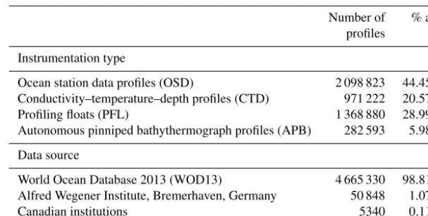
The WOD13 database (Boyer et al., 2013) (includ-ing the January 2017 update) served as the main data source for the WAGHC climatology. The profiles of the four instrumentation types were used: ocean sta-tion data (OSD), conductivity–temperature–depth (CTD), Argo profiling floats (PFL), and the autonomous pinniped bathythermograph data (APB). The latter were only used in the Southern Hemisphere where data coverage is generally poorer compared to the Northern Hemisphere. All four data types normally report both temperature and salinity. As both of these parameters are required for the spatial interpolation on isopycnal surfaces, the expendable (XBT) and mechani-cal (MBT) bathythermograph data were not used. We then added 50 848 profiles obtained from the Alfred Wegener In-stitute, Bremerhaven, and 5340 profiles received from dif-ferent institutions in Canada to the existing 4 665 330 tem-perature/salinity profiles from the WOD13. These two addi-tional datasets helped to significantly improve the data basis for northern polar regions. Table 1 gives details regarding the data types and data sources that contributed to the WAGHC. The dismissal of some instrumentation types along with the stringent quality control criteria explain why the total number of retained profiles is less than the approximate 5.4 million salinity profiles available in the WOD13 archive.
Figure 1 shows the yearly number of profiles of each data type retained after quality control. Before 1990 OSD profiles prevail, whilst CTDs are the main data type between 1990 and 2003. In later years, observations were mostly delivered by Argo floats, with the implementation of Argo floats being marked by a step-like increase in the number of available data.
Table 1.Instrumentation types and data sources that contributed to the WAGHC climatology.
Number of % all profiles
Instrumentation type
Ocean station data profiles (OSD) 2 098 823 44.452
Conductivity–temperature–depth profiles (CTD) 971 222 20.570
Profiling floats (PFL) 1 368 880 28.992
Autonomous pinniped bathythermograph profiles (APB) 282 593 5.985
Data source
World Ocean Database 2013 (WOD13) 4 665 330 98.810
Alfred Wegener Institute, Bremerhaven, Germany 50 848 1.077
Canadian institutions 5340 0.113
ALL
0 50 100 150 200 250
N*10³
1920 1930 1940 1950 1960 1970 1980 1990 2000 2010 2020 Year
OSD CTD PFL APB
Figure 1.Yearly number of profiles for each data type.
no or insufficient data, meaning that older data (since 1925) were utilized. However, the time frame for the data selection was narrower, especially within the upper 2 km Argo float depth range.
4 Data quality control procedure
Quality control is important for the construction of the clima-tology. Due to the large volume of data, an automated quality control (AQC) procedure was developed. It consists of a suite of the following quality checks:
1. crude parameter range check, 2. spike check,
3. constant value check, 4. multiple extrema check, 5. vertical gradient range check, 6. local climatological range check,
7. sample depth vs. local digital bathymetry check, 8. percentage of rejected (flagged) observed levels.
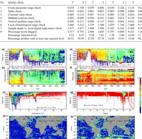
Before quality control, the observed depth levels were checked and reordered in increasing order if necessary. For the purpose of the initial tuning of the AQC procedure and for the final assessment of data quality, a diagnostic tool was developed which provides the statistics of rejected (flagged) data vs. time, observation depth, and bottom depth. The AQC procedure is applied to original profile data separately for temperature and salinity. Table 2 contains statistics of the data rejection rates. According to the statistics, Argo float data are characterized by the lowest rejection rate, followed by CTD, OSD, and APB data. The application of the local climatological range check and the sample level depth vs. lo-cal bathymetry quality checks results in the largest percent-ages of outliers.
Table 2.Data rejection rate for the automated quality control procedure.
Data type
OSD CTD PFL APB
Percent rejected levels
No. Quality check T S T S T S T S
1 Crude parameter range check 0.078 1.740 0.059 0.886 0.030 0.320 3.118 0.640
2 Spike check 0.010 0.003 0.001 0.001 0.005 0.008 0.004 0.003
3 Constant value check 0.004 0.114 0.007 0.114 0.004 0.128 0.024 0.043
4 Multiple extrema check 0.092 0.009 0.056 0.043 0.062 0.074 0.129 0.046
5 Vertical gradient range check 0.050 0.213 0.069 0.147 0.023 0.044 0.042 0.093 6 Local climatological range check 2.669 5.533 2.375 3.180 1.079 1.746 7,088 9.170 7 Sample depth vs. local digital bathymetry check 2.877 2.877 3.588 3.588 0.165 0.163 9.268 9.268
8 Percentage levels flagged 5.517 0.793 2.048 2.645 0.197 0.680 8.421 7.204
Percentage rejected levels 5.52 9.55 5.88 7.61 1.30 2.06 16.98 17.78
Percentage profiles with at least one rejected level 20.52 29.99 23.98 27.78 14.09 15.93 35.69 50.13
−7000 −6000 −5000 −4000 −3000 −2000 −10000 Depth (m)
Bin size = 1 year x 50 m
(a) 0 5 10 15 20 25 30 35 Temperature ( +O C)
1930 1940 1950 1960 1970 1980 1990 2000 2010 Year
Bin size = 1 year x 0.1oC
(b) −7000 −6000 −5000 −4000 −3000 −2000 −10000 Depth (m)
0 5 10 15 20 25 30 Temperature (+OC)
Bin size=0.1oC x 50 m
(c)
−160˚ −120˚ −80˚ −40˚ 0˚ 40˚ 80˚ 120˚ 160˚ −80˚ −60˚ −40˚ −20˚ 0˚ 20˚ 40˚ 60˚ 80˚
Bin size=1 oLATx1 LONGo
Longitude Latitude (d) −7000 −6000 −5000 −4000 −3000 −2000 −10000 Depth (m)
Bin size = 1 year x 50 m
(e) 0 5 10 15 20 25 30 35 40 45 Salinity (psu)
1930 1940 1950 1960 1970 1980 1990 2000 2010 Year
Bin size = 1 year x 0.1 psu (f) −7000 −6000 −5000 −4000 −3000 −2000 −10000 Depth (m)
0 5 10 15 20 25 30 35 40 Salinity
Bin size=0.1 psu x 50 m
(g)
−160˚ −120˚ −80˚ −40˚ 0˚ 40˚ 80˚ 120˚ 160˚ −80˚ −60˚ −40˚ −20˚ 0˚ 20˚ 40˚ 60˚ 80˚
Bin size=1 oLATx1 LONGo
Longitude Latitude (h) −1 2 5 10 20 50 100 %flagged
Figure 2.Temperature(a–d)and salinity(e–h)data rejection rates (all instrument types).
5 Vertical interpolation and extrapolation of the temperature and salinity profiles
The quality-controlled observed temperature and salinity profiles were finally interpolated on 65 unevenly spaced “standard” levels between the surface and 6750 m. The depth interval between the levels increased linearly with depth,
threshold value h: h=20 m within the upper 50m layer,
h=20+0.24·zbetween 50 and 2000 m (zis the mean dis-tance between the two levels in meters), and h=500 m for
z >2000 m. The limitation on the spacing between the ob-served levels is necessary to minimize the creation of artifi-cial water masses due to the interpolation procedure.
After the mid-2000s, the majority of the tempera-ture/salinity profiles come from Argo floats (Fig. 1). Since the floats only measure within the upper 2000 m layer, a step-like decrease in the data coverage occurs around the 2000 m level, which would create a strong bias towards the observa-tions above 2000 m when spatial interpolation is performed on isopycnal surfaces. To avoid this artifact, the profile exten-sion method was developed. The method is based on the ob-servational fact that the local temperature and salinity values are fairly constant below the main thermocline. First, in the vicinity of each profile potentially suitable for extrapolation, up to 10 deep CTD and OSD profiles are selected and the av-erage deep profile is calculated using distance weighted mean values at each standard level (the influence radius for the deep profile selection does not exceed 333 km). For the last observed levelZm(the merging depth) of the profiles subject
to extrapolation the temperature and salinity offsets (DToand
DSo) relative to the mean profile are calculated. If the
pa-rameter offset for the merging depth does not exceed a pre-defined threshold value (0.05◦C for temperature and 0.01 for salinity), and ifZm>1898 m (the deepest WAGHC standard
depth level within the Argo depth range), the profile is con-sidered to be suitable for extrapolation. The average profile is then modified as follows: at each depth levelZ > Zmthe
off-set value DP=DPo[1−(Z−Zm)/(Zmax−Zm)] is subtracted
from the average parameter value (temperature or salinity). The modified mean profile is used to extrapolate the original profile below the levelZm.
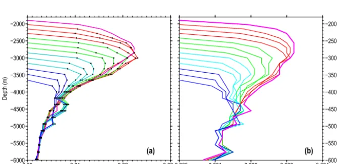
Figure 3 illustrates the extrapolation procedure for three arbitrarily selected full-depth CTD profiles. In order to esti-mate the average extrapolation error, we selected 52 672 full-depth CTD and OSD profiles deeper than 2200 m obtained after 1984 and interpolated on standard levels. The extrap-olation procedure was then applied to all of these profiles truncated at levels equal to or deeper than 1898 m. The re-spective mean absolute difference between the extrapolated and the original full-depth profile decrease with depth and are in the range between 0.03◦C at 3000 m and 0.002◦C at 6000 m for temperature and between 0.003 psu and 0.001 psu for salinity (Fig. 4).
Finally, the extrapolation procedure was applied to 720 839 quality controlled OSD, CTD, and PFL profiles that were obtained after 1984 and had their last level at or deeper then 1898 m. For most of the ocean area, the percentage of extrapolated levels exceeds 20 % from the total number of levels, with Argo extrapolated profiles comprising the largest group. The spatial distribution of full-depth and extrapolated profiles is shown in Fig. 5 along with the percentage of the interpolated levels and extrapolated profile frequency
distri-butions vs. the number of extrapolated levels and the year of observation.
6 Temporal and spatial data binning
The significantly increased data basis since the introduction of the Argo floats permits a better temporal and spatial reso-lution compared to the earlier WOCE Global Hydrographic Climatology (WGHC) (Gouretski and Koltermann, 2004). For each standard depth surface, the quality controlled ver-tically interpolated/extrapolated data were gridded by bin-averaging the data separately for each calender month in each 1/4◦grid cell. The binning procedure serves two purposes. Firstly, the binning reduces the overall number of observa-tions and, secondly, it reduces noise in the data. The thin-ning of the input profiles permits the application of the clas-sical optimal interpolation method without the use of a fast multiscale optimal interpolation algorithm proposed by Men-emelis et al. (1997).
With the aim of producing a climatology for the most data abundant recent years, the data selection for each spatial bin was performed iteratively, with the data being selected first for the time period from 1985 to 2016; thus, the WOCE hydrographic survey was embedded in the analysis. If no data were available for a particular grid node, the time pe-riod was extended to 1957–2016. For a small fraction of the grid nodes, all data since 1925 were used to produce the bin-averaged values. The percentage of spatial monthly bins pop-ulated with two or more observations decreased from 30 % in the upper several hundred meters to about 20 % at levels deeper than 2000 m.
The mean climatological year changes with depth, in the range from 2007 to 2011. For the upper 2 km layer where the Argo float data prevail, the climatological year is within the 3-year range between 2009 and 2011 (Fig. 6). Below the Argo depth range, the mean year is within the range from 2007 to 2009. Differences between the mean clima-tological year for different calendar months do not exceed 1 year. It is important to mention that the WOA13 clima-tology is created by averaging six decadal climatologies be-tween 1955 and 2012, with 1984 being the median year. This method prevents biases toward more recent and data abun-dant years. The difference between the median years of both climatologies does contribute to the temperature and salinity differences of the two gridded products and is discussed later in the text.
7 Spatial interpolation
−5000 −4500 −4000 −3500 −3000 −2500 −2000 −1500
Depth (m)
0.2 0.4 0.6 0.8 1.0 1.2 1.4 1.6 1.8 2.0 2.2 2.4 2.6 2.8 3.0 3.2 3.4 3.6 Temperature (oC)
A B
C
(a) A
B
C
−5000 −4500 −4000 −3500 −3000 −2500 −2000 −1500
Depth (m)
34.50 34.55 34.60 34.65 34.70 34.75 34.80 34.85 34.90
Salinity (psu) Observed profile
Mean profile
Shifted mean profile Offset at merging depth
A B
C
(b)
Figure 3.Example of the profile extrapolation procedure for three arbitrarily selected CTD temperature(a)and salinity(b)profiles.
−6000 −5500 −5000 −4500 −4000 −3500 −3000 −2500 −2000
Depth (m)
0.00 0.01 0.02 0.03
Temperature difference (oC) (a)
−6000 −5500 −5000 −4500 −4000 −3500 −3000 −2500 −2000
Depth (m)
0.000 0.001 0.002 0.003 0.004 Salinity difference (psu)
(b)
Figure 4.Mean absolute difference between the observed and extrapolated profiles for temperature(a)and salinity(b)at different merging depths. The intersection of each difference profile with theyaxis corresponds to the respective merging depth.
here in the form suggested by Gandin (1963). For the opti-mal interpolation on isobaric surfaces, the noropti-malized spatial covarianceCxyhof temperature and salinity was represented through the negative squared exponential:
Cxyh=exp− h
(rx/Lx)2+ ry/Ly2+(h/H )2 i
, (1)
whererxandryare zonal and meridional distances between the two points, LxandLyare the zonal and meridional
Figure 5. (a)Positions of full-depth profiles used for the extrapola-tion procedure (blue – before 1985, red – after 1984);(b)positions of extrapolated profiles (red – Argo profiles, blue – non-Argo pro-files);(c)percentage of extrapolated levels;(d)extrapolated profile frequency distribution vs. the number of extrapolated levels; and (e)extrapolated profile frequency distribution vs. the year of obser-vation.
was set to 2 km. Based on the evaluation of the test calcula-tions the signal-to-noise variance ratio was chosen to be 0.5 as a trade-off between the smoothness and desirable feature resolution.
For the optimal interpolation on isopycnal surfaces the normalized spatial covariance Cxyz was also represented through the negative squared exponential:
Cxyz=exp− h
(rx/Lx)2+ ry/Ly
2
+(</Z)2i, (2)
where<is the depth difference between the vertical positions of the same isopycnal surface, andZ=250 m is the decorre-lation depth scale. The introduction of this term is aimed at reducing the depth bias that appears near the boundaries of the domain, where observations are biased to one side (above or below) of the analyzed grid level. The objective analysis is performed on deviations between the observations and first guess values. To provide the distance-weighted means for the first guess temperature, salinity, and density fields, Eq. (1) was used withLxandLyset to 555 km.
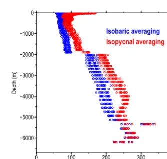
The spatial covariances of the analyzed temperature and salinity fields should be derived from available observations. However, the correlation length scale must at least be larger than the data spacing (Nuss and Tutley, 1994; Sokolov and Rintoul, 1999). We use the mean average distance to the four nearest bin-averaged neighbor profiles as the measure of data sparseness (Fig. 7). The distance between the observation points increases with depth from about 70–100 km within the upper 2000 m to about 200–300 km in the lower layer. These mean values were used as a guide for the choice of the decorrelation length scale for the optimum interpolation. Af-ter some experimenting, we decided on a decorrelation scale value of 333 km, which was used at all levels for the cur-rent version of the climatology (the decorrelation scale is the distance at which the autocorrelation function decreases to
−6000 −5000 −4000 −3000 −2000 −1000 0
Depth (m)
2006 2008 2010 2012 2014
Mean year
Figure 6.Area-mean climatological year vs. depth. Monthly values above 1900 m are shown in red.
−6000 −5000 −4000 −3000 −2000 −1000 0
Depth (m)
0 100 200 300 400
Mean distance to four nearest observations (km) Isobaric averaging Isopycnal averaging
Figure 7. The mean average distance to the four nearest bin-averaged profiles vs. depth.
1/e times the value of the zero lag). As noted by Sokolov and Rintoul (1999), the optimal interpolation produces a spa-tial average of the analyzed parameters, acting as a low-pass filter.
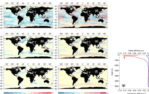
Figure 8.Temperature(a–c)and salinity(d–f)differences between the isopycnally averaged and isobarically averaged WAGHC climatolo-gies for selected depth levels in January: 150 m(a, d), 518 m(b, e), 1050 m(c, f); and area-averaged differences vs. depth(g).
At each grid location, the stabilized isobarically averaged density profile defines the set of local density surfaces on which the interpolation of temperature is subsequently per-formed. As in the isobaric case, the salinity is inferred from density and temperature values.
The advantage of the isobaric method is that it can be applied in exactly the same way throughout the water col-umn. However, the averaging (smoothing) of data along lev-els of constant depth does not correspond to the process of the water mass mixing in the real ocean which takes place along isopycnal, or more correctly along the neutral density surfaces. In contrast, the isopycnal averaging does not pro-duce artificial water masses; however, in the regions where isopycnals outcrop at the surface or bottom, the isopycnally averaged parameters are biased toward the ocean interior (Schmidtko et al., 2013).
8 Isobarically averaged vs. isopycnally averaged WAGHC climatology
Differences between parameter distributions on selected levels between the isopycnally and isobarically averaged WAGHC climatologies are shown in Fig. 8a–e. As expected the largest differences occur in regions of strong spatial
tem-perature and salinity gradients, like the Gulf Stream, the Kuroshio, Antarctic Circumpolar Current, and the equato-rial and tropical Pacific Ocean. In such regions the abso-lute difference in temperature and salinity can exceed 1◦C and 0.2 psu, respectively. The differences diminish with in-creasing depth. Thus, at the level of 1050 m, only the North Atlantic and the belt of the Antarctic Circumpolar Current show systematic differences exceeding 0.05◦C and 0.01 psu for temperature and salinity, respectively. Integrated over the whole ocean area (Fig. 8g), the climatological isobaric tem-perature values are higher than the isopycnally averaged val-ues. The same is true for the salinity except for the upper 100 m layer. Below 2000 m, typical absolute differences be-tween the isobarically and isopycnally averaged temperature and salinity values remain below 0.25◦C and 0.005 psu, re-spectively.
9 WAGHC vs. WOA13 climatology
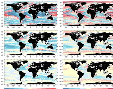
clima-Figure 9.Temperature(a–c)and salinity(d–f)isopycnal WAGHC climatology minus WOA13 climatology differences for selected depth levels in January: 150 m(a, d), 518 m(b, e), and 1050 m(c, f).
tology was used, below this level we used the annual WOA13 temperature and salinity fields.
9.1 Temperature and salinity distributions at levels As previously noted, the interpolation in WOA13 is per-formed on isobaric surfaces for temperature and salinity sep-arately, so that similar difference patterns can be identi-fied as in the case of isobarically and isopycnally averaged WAGHC climatologies. Indeed, Figs. 8a–f and 9a–f reveal several qualitatively similar patterns, indicating the largest differences in the areas with strong spatial gradients. We note that part of the differences should be attributed to climate change, since both climatologies are about 27 years apart on average. As progressive warming has been observed for the global ocean over the last few decades, Fig. 9a–f in contrast to Fig. 8a-f are dominated by the regions with positive tem-perature differences. These differences are described in more detail later in this paper. The introduction of the third term in Eq. (2) effectively reduces the depth bias near the bound-aries, so that the differences in temperature and salinity in Fig. 8 are mostly due to the interpolation method.
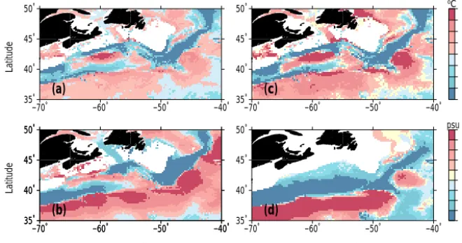
The temperature and salinity differences between the isopycnal and isobaric versions of the WAGHC climatology
at 150 m level for part of the northwestern Atlantic Ocean are shown in Fig. 10a and b. Here, along the path of the Gulf Stream, very high lateral temperature and salinity gradients occur with the effect of the data averaging method being especially pronounced. Parameter differences between the WAGHC and the WOA13 climatologies for the same level are presented in Fig. 10c and d. A very good agreement be-tween the respective difference fields is clearly seen, suggest-ing that the differences between the WAGHC and WOA13 climatologies are mostly due to the difference in the interpo-lation method. Recently, the NCEI produced several regional climatologies including the Northwest Atlantic Regional Cli-matology (Seidov et al., 2016) with 0.1◦resolution. A com-parison with this climatology might reduce the discrepancies but remains beyond the scope of the present study.
9.2 Differences in temperature–salinity space
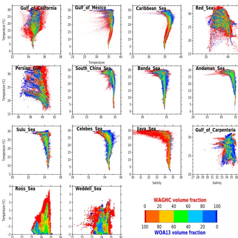
The differences between the WAGHC and the WOA13 at-las can be further identified using the volume T–S di-agrams. For each bin the volume ratio r=(VWOA13−
VWAGHC)/(VWOA13+VWAGHC) was calculated giving the
grid-−70˚ −60˚ −50˚ −40˚ 35˚
40˚ 45˚ 50˚
(a)
Latitude
−70˚ −60˚ −50˚ −40˚
35˚ 40˚ 45˚ 50˚
(b)
−70˚ −60˚ −50˚ −40˚
35˚ 40˚ 45˚ 50˚
Longitude
Latitude
−70˚ −60˚ −50˚ −40˚
35˚ 40˚ 45˚ 50˚
(c)
−9.0 −1.0 −0.5 −0.2 0.0 0.2 0.5 1.0 9.0 oC
−70˚ −60˚ −50˚ −40˚
35˚ 40˚ 45˚ 50˚
(d)
−9.00 −0.16 −0.08 −0.04 −0.01 0.01 0.04 0.08 0.16 9.00 psu
Longitude
Figure 10.Temperature(a)and salinity(b)differences between the isopycnally averaged and isobarically averaged WAGHC climatology in the northwestern Atlantic at the 150 m level in January;(c, d)same but for the isopycnally averaged WAGHC minus WOA13 differences.
0 5 10 15 20 25 30
Temperature [
oC]
0 5 10 15 20 25 30 35 40
0−500 m
0 5 10 15 20 25
32 34 36 38 40 42
500−1000 m
0 5 10 15 20 25
32 34 36 38 40 42
1000−1500 m
0 2 4 6 8
Temperature [
oC]
34.0 34.5 35.0 35.5 36.0
Salinity 1500−2500 m
−1 0 1 2 3 4 5
34.6 34.7 34.8 34.9 35.0
Salinity 2500−3500 m
−1 0 1 2 3 4 5
34.6 34.7 34.8 34.9 35.0
Salinity 3500−6500 m
0 20WAGHC volume fraction40 60 80 100
100 80 60 40 20 0
WOA13 volume fraction
Figure 11.T–Shistograms for six depth layers of the world ocean. Bin sizes are 0.05◦C for temperature and 0.005 for salinity. Histograms are based on the gridded WAGHC and WOA13 climatologies. Colors represent the volume fraction of each climatology.
ded data for six selected depth layers are shown in Fig. 11. The largest differences between the two climatologies are found within the upper 1500 m layer, with the WOA13 usually showing broader T–S sequences compared to the WAGHC climatology. Unrealistically high WOA13 salinities exceeding 35.5 psu are found in the temperature range below
2◦C. A generally good agreement is observed for the layers
below 1500 m where the WOA13 climatology is represented by the annual temperature and salinity fields.
de-Figure 12. Selected areas within the world ocean for whichT–S histograms have been compared between the WAGHC and WOA13 climatologies. Please note that the above figure contains disputed territories.
scribe the most pronounced differences revealed by the T–
S diagrams for particular areas (Fig. 13a and b). Unfortu-nately, it is not possible to give a definite explanation for these differences, as many details regarding the construction of the WOA13 are not known to us. For the Arctic Ocean without the marginal seas, the WOA13 climatology produces unrealistically high salinities exceeding 36 psu. In contrast, for Baffin Bay, the Kara Sea, the White Sea and the Euro-pean Nordic seas, WOA13 gives much lower salinities com-pared to the WAGHC climatology. For temperatures below ca. 2◦C, the WOA13 climatology gives unrealistically high salinities for the Kara Sea, the White Sea, and Hudson Bay. At least part of the differences described above can be at-tributed to the much poorer WOA13 data basis for the north-ern polar region compared to the WAGHC.
Significantly different T–S diagrams are also found for several of the data abundant regions. For instance the Baltic Sea is characterized by extraordinarily good data coverage. However, significant deviations between the two climatolo-gies are clearly seen: (1) the waters with salinities below 5 psu are completely absent in the WOA13; and (2) salini-ties higher than 25 psu are not known for the Baltic Sea but are present in the WOA13 climatology. Very different T–S
diagrams are found for the Caspian Sea. Here, the WOA13 gridded fields report salinities lower than 7 psu throughout the whole temperature range, along with unrealistically high temperatures exceeding 30◦C. For the Mediterranean Sea the WOA13 gridded product exhibits low-salinity sequences (below 36.5 psu) that are not supported by the observational
data. In the Pacific Ocean we note the unrealistically broad WAGHC salinity range for the Sea of Okhotsk, especially for the deep waters with temperatures below 5◦C. TheT–S di-agrams for the two climatologies differ considerably for the Gulf of California. Here the WOA13 climatology exhibits a very broad salinity range even for the deep part of the wa-ter column, with temperatures below 12◦C where theT–S
relation becomes very tight. Similar to the Gulf of Califor-nia, we find WOA13 salinity ranges that are too broad in the deep waters of the Gulf of Mexico and the Caribbean Sea. The WOA13 climatology is also biased to low upper layer salinities in the Andaman and Java seas. Finally, we note a broader WOA13 salinity range for the Weddell Sea. Here, the WOA13 climatology gives unrealistically high salinities exceeding 35 psu, in disagreement with observations. 9.3 Volume-averaged temperature and salinity
differences
As noted above, the spatial patterns of temperature and salin-ity differences at selected levels between the isopycnally averaged WAGHC climatology and isobarically averaged WOA13 climatology resemble the differences between the isopycnally and isobarically averaged WAGHC climatolo-gies, suggesting the dependence on interpolation method.
0 5 10 15 20 25 30 Temperature ( oC)
0 5 10 15 20 25 30 35 40
World_ocean
0 5 10 15
0 5 10 15 20 25 30 35 40
Arctic_Ocean −2 0 2 4 6 8 10
20 25 30 35
Baffin_Bay −2 0 2 4 6 8 10
0 5 10 15 20 25 30 35 40
Kara_Sea 0 5 10 15 Temperature ( oC)
15 20 25 30 35
White_Sea
0 5 10 15
20 25 30 35
European_Nordic_seas 0 5 10 15 Temperature
0 5 10 15 20 25 30 35 40
Hudson_Bay 0 5 10 15 20
15 20 25 30 35 40
Gulf_of_Saint_Lawrence 0 5 10 15 20 Temperature ( oC)
20 25 30 35 40
North_Sea 0 5 10 15 20 25
0 5 10 15 20 25 30 35
Baltic_Sea
5 10 15 20
32 33 34 35 36
Irish_Sea 0 5 10 15 20 25 30
0 5 10 15 20
Azov_Sea 0 5 10 15 20 25 Temperature ( oC)
10 15 20 25
Black_Sea 0 5 10 15 20 25 30
0 5 10 15 20
Caspian_Sea 10 15 20 25 30 35 40 Mediterranean_Sea 10 15 20 25 30
32 34 36 38 40 42
Adriatic_Sea 5 10 15 20 25 Temperature ( oC)
15 20 25 30 35 40
Salinity Marmara_Sea 0 5 10 15
15 20 25 30 35
Salinity Sea_of_Okhotsk 0 5 10 15 20 25 30
26 28 30 32 34
Salinity Yellow_Sea 0 5 10 15 20 25 30
25 30 35
Salinity
Sea_of_Japan
0 5 10 15 20 25 30 Temperature ( oC)
32 34 36 38
Gulf_of_California 0 5 10 15 20 25 30
20 25 30 35 40
Temperature Gulf_of_Mexico 0 5 10 15 20 25 30
25 30 35 40
Caribbean_Sea 15 20 25 30 35 40 Red_Sea 15 20 25 30 Temperature ( oC)
36 38 40 42
Persian_Gulf 0 5 10 15 20 25 30
20 25 30 35
South_China_Sea 0 5 10 15 20 25 30 30 35 Banda_Sea 0 5 10 15 20 25 30
20 25 30 35
Andaman_Sea 5 10 15 20 25 30 Temperature ( oC)
30 32 34 36
Sulu_Sea 0 5 10 15 20 25 30
30 32 34 36
Celebes_Sea 0 5 10 15 20 25 30
30 31 32 33 34 35 36
Salinity
Java_Sea
20 25 30
27 28 29 30 31 32 33 34 35 36 37 Salinity Gulf_of_Carpentaria −2 −1 0 1 2 3 4 Temperature ( oC)
31 32 33 34 35 36
Salinity Ross_Sea −2 −1 0 1 2 3 4
31 32 33 34 35 36
Salinity
Weddell_Sea
0 20 40 60 80 100
WAGHC volume fraction
100 80 60 40 20 0
WOA13 volume fraction
Figure 13.T–Shistograms for selected areas of the world ocean (see Fig. 12) for WAGHC and WOA13 gridded climatologies. Bin size is 0.1◦C×0.05 psu. Colors represent the volume fraction of each climatology. Please note that the above figure contains disputed territories.
WAGHC climatology as being warmer and saltier on aver-age. A rather pronounced dependence on latitude is observed, with “tounges” of positive differences linked to the Antarctic Circumpolar Current and to latitudes north of 30◦N.
The mean temperature difference for the 0–300, 0–700, and 0–1500 m layers are 0.127, 0.079, and 0.048◦C, respec-tively. We attribute these differences to real changes in the world ocean over an approximate 25-year time period be-tween the WAGHC and WOA13 climatologies. The time difference plot (Figs. 14c and 15c) was produced assuming
1984 as the median year for the WOA13 climatology, which was created as the average of six decadal climatologies. 9.4 Annual cycle
−1400 −1200 −1000 −800 −600 −400 −200 0 Depth (m)
−60 −40 −20 0 20 40 60 Latitude −10.00 −0.30 −0.20 −0.10 −0.05 0.00 0.05 0.10 0.20 0.30 10.00 oC (a) −1400 −1200 −1000 −800 −600 −400 −200 0
−60 −40 −20 0 20 40 60 Latitude −10.000 −0.200 −0.150 −0.100 −0.050 0.000 0.005 0.010 0.020 0.030 10.000 psu (b) −1400 −1200 −1000 −800 −600 −400 −200 0
−60 −40 −20 0 20 40 60 Latitude 15 17 19 21 23 25 27 Year (c)
Figure 14.Zonally averaged differences between the WAGHC and WOA13 climatologies for temperature(a), salinity(b), and mean clima-tological year(c).
−1500 −1000 −500 0
Depth (m)
0.0 0.1 0.2 0.3
TWAGHC−TWOA13
Mean=0.048oC
(a) −1500 −1000 −500 0
−0.01 0.00 0.01 0.02 0.03 SWAGHC−SWOA13
Mean=0.0017 psu (b) −1500 −1000 −500 0
20 25 30
YEARWAGHC−YEARWOA13
Mean=24.9 years
(c)
Figure 15.Differences between the WAGHC and WOA13 climatologies vs. depth for temperature(a), salinity(b), and for the mean clima-tological year(c).
Pacific oceans and in the tropical and equatorial belts. Max-imum salinity amplitudes are observed in the polar ocean and in several tropical areas like the Indonesian seas and the northern Indian Ocean. The difference plots for temperature (Fig. 16e) are characterized by higher WAGHC amplitudes in the tropical belt, the Gulf Stream, off northeastern Greenland, and within the Agulhas Return Current. The difference plot for salinity (Fig. 16d) generally shows much higher WAGHC amplitudes for the polar ocean and for the eastern tropical Pa-cific Ocean.
The zonally averaged September minus March differences shown in Fig. 17 are very similar to the plots based on Argo data and presented by Roemmich and Gilson (2009), and confirm the hemispheric asymmetry with seasonal ampli-tude in the Northern Hemisphere being much higher com-pared to the Southern Hemisphere. However, several sys-tematic differences between the climatologies may be noted. The WAGHC climatology gives a 0.5◦C higher temperature amplitude near the Equator within the depth layer from 50 to 100 meters. In comparison, the WAGHC climatology be-tween 10 and 80◦N is characterized by a 0.2–0.5◦C lower amplitude in the seasonal cycle. The annual cycle differences between the climatologies for salinity are less pronounced, with the largest differences found in the polar latitudes of both hemispheres.
9.5 Ocean heat content time series
Finally, we used the WAGHC and WOA13 climatologies to test them as the baseline mean for the calculations of the ocean heat content anomaly (OHCA) time series.
Here the OHCA time series between 1920 and 2016 (Fig. 18) were calculated as follows. First, the depth aver-aged temperatures for the 0–300 and 0–700 m layers were obtained. The mean layer temperature anomaly was then dif-ferenced from a baseline climatological monthly mean. The global temperature anomaly for each layer was represented as the area-weighted mean of all 1◦latitude zones containing data. For each 1◦ zone, the temperature anomaly was rep-resented by the mean of all 1◦ boxes containing data. The calculated global temperature anomalies were converted to OHCA over the entire ocean area. This was equivalent to the assumption that the mean temperature anomaly for the ocean boxes without data was equal to the mean anomaly estimated for the grid boxes with observations. We note that the time se-ries presented in Fig. 18 represent the decadal mean anoma-lies centered on each calendar year. Figure 18c–i shows tem-perature anomalies averaged for selected decades in 1×1◦ boxes.
Figure 16.Annual cycle amplitudes for temperature (a– WAGHC,b– WOA13) and salinity (d– WAGHC,e– WOA13) averaged over the upper 100 m layer for the WAGHC and WOA13 climatologies. Amplitude difference WAGHC minus WOA13 for temperature(c)and salinity(f).
−400 −300 −200 −100 0
Depth (m)
(a) (b) (c) −8.0−4.0
−2.0 −1.0 −0.5 −0.2 0.0 0.2 0.5 1.0 2.0 4.0 6.0 8.0 12.0
psu
−400 −300 −200 −100 0
Depth (m)
−80−60−40−20 0 20 40 60 80 (d)
Latitude
−80−60−40−20 0 20 40 60 80 (e)
Latitude
−80−60−40−20 0 20 40 60 80 (f)
Latitude
−2.50 −1.50 −0.50 −0.20 −0.10 −0.05 0.00 0.05 0.10 0.20 0.50 1.50
oC
Figure 17.Zonally averaged September minus March differences vs. depth for(a)WAGHC temperature,(b)WOA13 temperature;(c) dif-ferencea−b;(d)WAGHC salinity;(e)WOA13 salinity; and(f)differenced−e.
synthesis (German contribution to Estimating the Circula-tion and Climate of the Ocean) (Köhl and Stammer, 2008). This method was previously applied to the upper-ocean tem-perature anomaly calculations (Gouretski et al., 2012). The GECCO synthesis provides an estimate of ocean circulation
Figure 18.Decadal globally integrated ocean heat content anomaly (ZJ) time series for 1920–2016 for 0–300 m(a)and 0–700 m(b)layers computed using WAGHC (red curve) and WOA13 (blue curve) baseline climatologies. Error bars correspond to the errors due to the irreg-ular and incomplete sampling; the green line corresponds to the heat content change estimated by differencing the WAGHC and WOA13 climatologies.(c–j)The 0–300 m layer temperature anomalies in 1×1◦boxes averaged over the selected decades.
model output. The standard deviation of the difference be-tween the two time series provides the measure of uncertainty due to the irregular and incomplete sampling for that decade. Unfortunately, the historical climatologies are based on data irregularly distributed in time and space and can have different mean years for different regions of the ocean, which introduces inconsistencies among the regions. Boyer et al. (2016) used three monthly mean temperature clima-tologies to test the sensitivity of the OHCA estimates for the global ocean to the choice of the baseline mean. The OHCA uncertainty for the 0–700 m layer due to the baseline mean was found to depend on the mapping method and time pe-riods, varying between 2.7 and 24.5 ZJ, which corresponds to approximately 2 % to 16 % of the full OHCA range be-tween 1970 and 2010.
Our calculations reveal much smaller differences due to the choice of baseline mean. The largest differences reach about 10 % of the full OHCA range for some years be-tween 1920 and 2015 and are observed before the mid-1950s. This time period is characterized by an extremely uneven dis-tribution of observations and almost no observations in the Southern Hemisphere, especially during the 1940s. After the mid-1950s, the differences due to the baseline mean do not exceed a few percent.
We find an OHCA increase of∼150 ZJ since 1920 for the 0–300 m layer and of∼220 ZJ for the 0–700 m layer. Both time series are characterized by an acceleration of the ocean heat content growth since the mid-1990s. As mentioned in Sect. 9.3, the WAGHC and WOA13 climatologies have a mean year difference exceeding 25 years, meaning that the overall temperature differences between the two climatolo-gies can be attributed to climate change in the ocean over this time period. The overall temperature (OHCA) differences be-tween the two climatologies are shown in green in Fig. 18, and in both cases they are lower than the OHCA differences obtained from decadal time series (72 % and 89 % for the 0– 300 and 0–700 m layers, respectively).
10 Conclusions
basis. Two versions of the climatology are available, with the spatial interpolation being performed on isobaric and isopy-cnal surfaces, respectively.
The WAGHC climatology is further compared to the widely used 1/4◦resolution isobarically averaged climatol-ogy WOA13, produced by the NOAA Ocean Climate Labo-ratory (Locarnini et al., 2013). We note generally good agree-ment between these two gridded products. The differences between the two climatologies are basically attributed to in-terpolation method (isopycnal vs. isobaric averaging) and to the considerably improved data basis (the WAGHC includes an additional 4 years of the Argo float and other data). The in-clusion of additional data into the WAGHC climatology sig-nificantly improved the representation of the thermohaline structure in polar regions. However, a significant improve-ment was also achieved for several data abundant regions like the Baltic Sea, the Caspian sea, the Gulf of California, the Caribbean Sea, and the Weddell Sea. Further investigations are needed to identify the causes of differences between the two climatologies in these regions.
We also tested the dependence of the ocean heat content anomaly (OHCA) time series on the baseline climatology. Since the 1950s, both WAGHC and WOA13 used as baseline means produce almost identical OHCA time series. Even for the earlier data-poor decades, the largest differences do not exceed 10 % of the full OHCA range.
Appendix A: Quality control tests on temperature and salinity profiles
A1 Crude range check
The data are screened for extreme temperature and salin-ity values. Global temperature–depth and salinsalin-ity–depth his-tograms are used to define the respective masks for gross er-rors. Values falling outside the mask fail the test. It is as-sumed that observations which failed the test give no infor-mation on the true parameter values.
A2 Spike check
The check aims to identify spikes in temperature and salinity profiles. For each triple of parameter values on neighboring depth levelspk,pk+1,pk+2the following test values are
cal-culated:
s1= |pk+1−(pk+pk+2)·0.5| (A1)
s2= |(pk+2−pk)·0.5| (A2)
s=s1−s2. (A3)
If the value s exceeds the depth dependent threshold valuesmax, the levelk+1 is flagged. The test is not performed
for profiles with large gaps between the observed levels. A3 Constant value check
This test proves how many temperature/salinity measure-ments of one profile are identical. The test includes two tun-able parameters: the minimal thickness of the layer within which all measurements shows exactly the same parameter value, and the number of such levels within the layer. The first parameter sets the threshold thickness of the thermostad and halostad, whereas the second parameter takes the typical observed level spacing into account, which differs between instrumentation types.
A4 Multiple extrema check
This test identifies profiles with unrealistically large numbers of local parameter extrema. For each triple of three neighbor observed levels the extremum is considered to be significant if|pk−pk+1|< d and|pk−pk−1|< d, where the
parame-terd is selected to be larger than the measurement precision and the typical amplitude of the microscale parameter inver-sions.
A5 Vertical gradient range check
This test identifies pairs of levelskandk+1 for which the vertical gradients of temperature or salinity exceed the over-all depth dependent ranges. The gradient ranges are defined on the basis of the depth–gradient histograms. Both observa-tions are flagged when the vertical gradient falls outside the range.
A6 Local climatological range check
For the calculation of the climatological parameter ranges the adjusted box plot method for skewed distributions is used (Vanderviere and Huber, 2004). Here, the skewness of the local parameter distribution is taken into account, so that the local climatological range is defined as
[Q1−Hl(MC)IQR;Q3+Hr(MC)IQR], (A4) where Hl(MC)=1.5eaMC, Hr(MC)=1.5ebMC, Q1 and Q3 are the first and the third quartiles, respectively, and
IQR=Q3−Q1is the interquartile range.
The medcouple MC is defined as follows: MC(F )=medianh (x1, x2) , (x1<MF< x2) , and
h xi, xj= xj−mF−(mF−xi)/ xj−xi. (A5) At each 0.25◦ grid node and at each standard level, the lo-cal median and the medcouple were lo-calculated using data within a variable influence radius. The influence radius was increased iteratively from the initial value of 55 km to the limit of 333 km in order to achieve the target number of 300 observations.
A7 Sample depth vs. local digital bathymetry check For the local bathymetry check the 0.5 arcmin resolution dig-ital GEBCO bathymetry was used. Profiles situated on land according to the digital bathymetry were rejected. For the ocean profiles the levels deeper than the local bottom depth (added by the depth-dependent tolerance) were flagged and not used for the further analysis.
Competing interests. The author declares that he has no conflict of interest.
Acknowledgements. The ongoing efforts of the NOAA Ocean Climate Laboratory to prepare and disseminate the newest updates of the global hydrographic data archive which provided the main data basis for this study are highly appreciated. I am thankful to the Department of Fisheries and Oceans of Canada for the hydrographic data from the Arctic Ocean. I am also grateful for the hydrographic data from the North Atlantic collected by the Freshwater Institute, Bedford Institute of Oceanography, Institute Maurice-Lamontagne, Northwest Atlantic Fisheries Centre, and the Institute of Ocean Sciences. I would particularly like to thank Mathieu Ouellet, Colline Combault, and Ives Gratton for preparing these data for me. My thanks go to the colleagues from the Alfred Wegener Institute, Bremerhaven, especially to Axel Behrend, for sharing their collection of the Arctic hydrographic data with me. I am grateful to Marc Carson for careful reading of the paper and numerous suggestions for improvement. Finally, I would like to thank the colleagues from the German Climate Computing Center (DKRZ) for their help regarding the publication the WAGHC climatological gridded dataset. The two anonymous reviewers provided useful comments on an earlier version of this paper. This work was conducted as part of the Excellence Initiative CLISAP at the Universität Hamburg, funded through the German Science Foundation (Grant EXC 177/2).
Edited by: David Stevens
Reviewed by: two anonymous referees
References
Barnes, S. L.: A technique for maximizing detailes in numerical weather map analysis, J. App. Meteorol., 3, 396–409, 1964. Boyer, T., Levitus, S., Garcia, H., Locarnini, R., Stephens, C., and
Antonov, J.: Objective analyses of annual, seasonal, and monthly temperature and salinity for the World Ocean on 0.25◦grid, Int. J. Climatol., 25, 931–945, 2005.
Boyer, T., Antonov, J., Baranova, O., Coleman, C., Garcia, H., Grodsky, A., Johnson, D., Locarnini, R., Mishonov, A., O’Brian, T., Paver, C., Reagan, J., Seidov, D., Smolyar, I., Zweng, M., Levitus, S. (Ed.), and Mishonov, A. (Technical Ed.): WORLD OCEAN DATABASE 2013, NOAA Atlas NESDIS 72, US Gov-ernment Printing Office, Washington, D.C., 209 pp., 2013. Boyer, T., Domingues, C. M., Good, S., Johnson, G., Lyman,
J., Ishii, M., Gouretski, V., Willis, J., Antonov, J., Wijf-fels, S., Church, J., Cowley, R., and Bindoff, N.: Sensitivity of Global Upper-Ocean Heat Content Estimates to Mapping Methods, XBT Bias Corrections, and Baseline Climatologies, J. Climate, 29, 4817–4842, https://doi.org/10.1175/JCLI-D-15-0801.1, 2016.
Gandin, L.: Objective Analysis of Meteorological Fields, Gidrome-teorologicheskoe Izdatel’stvo, Leningrad, 242 pp., 1963. Gouretski, V.: WOCE-Argo Global Hydrographic Climatology
(WAGHC Version 1.0), World Data Center for Climate (WDCC) at DKRZ, https://doi.org/10.1594/WDCC/WAGHC_V1.0, last access: February 2018.
Gouretski, V. V. and Jancke, K.: Systematic errors as the cause for an apparent deep water property variability: global analysis of the WOCE and historical hydrographic data, Progr. Oceanogr., 48, 337–402, 2001.
Gouretski, V. V. and Koltermann, K. P.: WOCE Global Hydro-grahic Climatology, in: Berichte des BSH, 35, Bundesamt für Seeschiffsfahrt und Hydrographie, Hamburg, 52 pp., 2004. Gouretski, V. V., Kennedy, J., Boyer, T., and Köhl, A.: Consistent
near-surface ocean warming since 1900 in two largerly inde-pendent observing networks, Geophys. Res. Lett., 39, L19606, https://doi.org/10.1029/2012GL052975, 2012.
IOC, SCOR and IAPSO: The international thermodynamic equation of seawater 2010: Calculation and use of thermodynamic prop-erties, Intergovernmental Oceanographic Commission, Manuals and Guides No. 56, UNESCO, Paris, 196 pp., 2010.
Köhl, A. and Stammer, D.: Variability of the meridional over-turning in the North Atlantic from the 50 years GECCO state estimation, J. Phys. Oceanogr., 38, 1913–1930, https://doi.org/10.1175/2008JPO3775.1, 2008.
Koltermann, K. P., Gouretski, V. V., and Jancke, K.: Hydrographic Atlas of the orld Ocean Circulation Experiment (WOCE), in: Volume 3: Atlantic Ocean, edited by: Sparrow, M., Chapman, P., and Gould, J., Intrernational WOCE Project Office, Southamp-ton, UK, 2011.
Levitus, S.: Climatological Atlas of the World Ocean, US Gov. Printing Office, Washington, D.C., 173 pp., 1982. Levitus, S., Burgett, R., and Boyer, T. P.: World Ocean Atlas 1994,
in: Volume 3: Salinity, NOAA Atlas NESDIS 3, US Department of Commerce, Washington, D.C., 99 pp., 1994.
Levitus, S., Boyer, T., Conkright, M., O’Brian, T., Antonov, J., Stephens, C., Stathopulos, L., Johnson, D., and Gelfeld, R.: World Ocean Database 1998, in: Vol. 1: Introduction, NOAA Atlas NESDIS 18, US Gov. Printing Office, Washington, D.C., 346 pp., 1998.
Locarnini, R. A., Mishonov, A. V., Antonov, J. I., Boyer, T. P., and Garcia, H. E.: World Ocean Atlas 2005, in: Volume 1: Tempera-ture, NOAA Atlas NESDIS 61, edited by: Levitus, S., US Gov-ernment Printing Office, Washington, D.C., 182 pp., 2006. Locarnini, R. A., Mishonov, A. V., Antonov, J. I., Boyer, T. P.,
Gar-cia, H. E., Baranova, O. K., Zweng, M. M., and Johnson, D. R.: World Ocean Atlas 2009, in: Volume 1: Temperature, NOAA At-las NESDIS 68, edited by: Levitus, S., US Government Printing Office, Washington, D.C., 184 pp., 2010.
Locarnini, R. A., Mishonov, A. V., Antonov, J. I., Boyer, T. P., Garcia, H. E., Baranova, O. K., Zweng, M. M., Paver, C. R., Reagan, J. R., Johnson, D. R., Hamilton, M., and Seidov, D.: World Ocean Atlas 2013, in: Volume 1: Temperature NOAA At-las NESDIS 73, edited by: Levitus, S. and Mishonov, A., Silver Spring, MD, 40 pp., 2013.
Lozier, M. S., McCartnes, M. S., and Owens, W. B.: Anomalous anomalies in averaged hydrographic data, J. Phys. Oceanogr., 24, 2624–2638, 1994.
Reiniger, R. F. and Ross, K. C.: A method of interpolation with application to oceanographic data, Deep-Sea Res., 15, 185–193, 1968.
Roemmich, D. and Gilson, J.: The 2004–2008 mean and annual cycle of temperature, salinity, and steric height in the global ocean from the Argo Program, Prog. Oceanogr., 82, 81–100, https://doi.org/10.1016/j.pocean.2009.03.004, 2009.
Schmidtko, S., Johnson, G., and Lyman, J.: MIMOC: A global monthly isopycnal upper-ocean climatology, J. Geophys. Res., 118, 1658–1672, https://doi.org/10.1002/jgrc.20122, 2013.
Seidov, D., Baranova, O. K., Boyer, T., Cross, S. L., Mis-honov, A. V., and Parsons, A. R.: Northwest Atlantic Re-gional Ocean Climatology, in: NOAA Atlas NESDIS 80, edited by: Mishonov, A. V., Silver Spring, MD, 56 pp., https://doi.org/10.7289/V5/ATLAS-NESDIS-80 (dataset: https://doi.org/10.7289/V5RF5S2Q), 2016.
Sokolov, S. and Rintoul, S.: Some remarks on Interpolation of Non-stationary Oceanographic Fields, J. Atmos. Ocean. Tech., 16, 1434–1449, 1999.