www.clim-past.net/13/107/2017/ doi:10.5194/cp-13-107-2017
© Author(s) 2017. CC Attribution 3.0 License.
Biome changes in Asia since the mid-Holocene – an analysis of
different transient Earth system model simulations
Anne Dallmeyer1, Martin Claussen1,2, Jian Ni3,4,5, Xianyong Cao4,6, Yongbo Wang4,7, Nils Fischer1, Madlene Pfeiffer8, Liya Jin9, Vyacheslav Khon10,11, Sebastian Wagner12, Kerstin Haberkorn2, and Ulrike Herzschuh4,6
1Max Planck Institute for Meteorology, Bundesstraße 53, 20146 Hamburg, Germany
2Meteorological Institute, Centrum für Erdsystemforschung und Nachhaltigkeit (CEN), Universität Hamburg,
Bundesstraße 55, 20146 Hamburg, Germany
3Institute of Biochemistry and Biology, University of Potsdam, Maulbeerallee 3, 14469 Potsdam, Germany
4Alfred Wegener Institute Helmholtz Centre for Polar and Marine Research, Telegrafenberg A43, 14473 Potsdam, Germany 5State Key Laboratory of Environmental Geochemistry, Institute of Geochemistry, Chinese Academy of Sciences,
Lincheng West Road 99, 550081 Guiyang, China
6Institute of Earth and Environmental Science, University of Potsdam, Karl-Liebknecht-Straße 24–25,
14476 Potsdam, Germany
7College of Resource Environment and Tourism, Capital Normal University, Beijing 100048, China 8Alfred Wegener Institute Helmholtz Centre for Polar and Marine Research, 27568 Bremerhaven, Germany 9Key Laboratory of Western China’s Environmental Systems, College of Earth and Environmental Sciences,
Lanzhou University, Lanzhou 730000, China
10Institute of Geosciences, Christian-Albrechts Universität zu Kiel, Ludewig-Meyn-Str. 10–14, 24118 Kiel, Germany 11A. M. Obukhov Institute of Atmospheric Physics RAS, Pyzhevsky 3, 117019 Moscow, Russia
12Helmholtz Center Geesthacht, Institute for Coastal Research, 21502 Geesthacht, Germany
Correspondence to:Anne Dallmeyer ([email protected])
Received: 22 June 2016 – Discussion started: 7 July 2016
Revised: 13 January 2017 – Accepted: 18 January 2017 – Published: 9 February 2017
Abstract.The large variety of atmospheric circulation sys-tems affecting the eastern Asian climate is reflected by the complex Asian vegetation distribution. Particularly in the transition zones of these circulation systems, vegeta-tion is supposed to be very sensitive to climate change. Since proxy records are scarce, hitherto a mechanistic un-derstanding of the past spatio-temporal climate–vegetation relationship is lacking. To assess the Holocene vegetation change and to obtain an ensemble of potential mid-Holocene biome distributions for eastern Asia, we forced the diagnos-tic biome model BIOME4 with climate anomalies of dif-ferent transient Holocene climate simulations performed in coupled atmosphere–ocean(–vegetation) models. The simu-lated biome changes are compared with pollen-based biome records for different key regions.
In all simulations, substantial biome shifts during the last 6000 years are confined to the high northern latitudes and
the monsoon–westerly wind transition zone, but the tempo-ral evolution and amplitude of change strongly depend on the climate forcing. Large parts of the southern tundra are replaced by taiga during the mid-Holocene due to a warmer growing season and the boreal treeline in northern Asia is shifted northward by approx. 4◦in the ensemble mean, rang-ing from 1.5 to 6◦in the individual simulations, respectively. This simulated treeline shift is in agreement with pollen-based reconstructions from northern Siberia. The desert frac-tion in the transifrac-tion zone is reduced by 21 % during the mid-Holocene compared to pre-industrial due to enhanced precip-itation. The desert–steppe margin is shifted westward by 5◦
The different character and the interplay of these circulation systems as well as the connection to the tropical Pacific lead to strong climate variability and regionally very diverse cli-mate conditions in Asia (e.g. Lau et al., 2000; Wang, 2006; Ding and Wang, 2008). This is furthermore intensified by the complex Asian orography including vast mountain ranges, high-elevated plateaus as well as deep depressions, basins and large plains (Broccoli and Manabe, 1992).
The regional climate peculiarities are reflected in the mul-tifaceted vegetation distribution. The climate in the cold Arc-tic zones is too harsh for trees and this temperature limita-tion results in prominent transilimita-tion of deciduous and ever-green taiga to tundra and even ice deserts in northern Asia (Larsen, 1980). In contrast, the warm tropical climate regions and large parts of eastern China are affected by the monsoon systems leading to high annual rainfall rates that support the growing of tropical and warm temperate forests (Ramankutty and Foley, 1999). The monsoon-related diabatic heating and vertical uplift at the Himalayas induce strong subsidence of air north and west of the Tibetan Plateau, leading to dry cli-mate in central and western Asia (e.g. Rodwell and Hoskins, 1996; Duan and Wu, 2005). Coincidently with this transition from monsoonal influenced climate to dry (westerly wind dominated) climate, a transition zone of forest to steppe and steppe to desert forms in central East Asia. Particularly in the two transition zones, i.e. the temperature-limited taiga– tundra margin and the moisture-limited forest–steppe–desert transition area, vegetation is supposed to be very sensitive to climate change and strong feedbacks are expected in case of climate and vegetation shifts due to large environmental and biophysical changes (e.g. Feng et al., 2006, and references therein).
During the mid-Holocene, cyclic variations in the Earth’s orbit around the sun led to substantial changes in climate (Wanner et al., 2008). The monsoon circulations were en-hanced (Kutzbach, 1981; Shi et al., 1993; Fleitmann et al., 2003; Wang et al., 2005) and the high northern latitudes ex-perienced a much warmer summer climate (Sundqvist et al., 2010; Zhang et al., 2010). Pollen-based reconstructions for the mid-Holocene time slice show an influence of these cli-mate changes on the vegetation distribution. The northern treeline was shifted poleward accompanied by an expansion of the boreal forest (MacDonald et al., 2000; Bigelow et al., 2003). The forests in East Asia were extended, the steppe–
time slices (e.g. Yu et al., 2000). Vegetation trends – so far – have mostly been presented by trends of different taxa for single sites not depicting the regional vegetation trend appro-priately.
Large climate model intercomparison projects have been established to assess the mid-Holocene to pre-industrial cli-mate change and to validate the state-of-the-art clicli-mate mod-els against the mid-Holocene climate (e.g. Joussaume et al., 1999; Braconnot et al., 2007a, b). Some of these models only poorly reflect observed Asian climate (Zhou et al., 2009, and references therein) and, accordingly, the simulated Holocene climate strongly deviates among the models and from recon-structions. Current Earth system models generally include interactively coupled dynamic vegetation models that are based upon comparable routines but differ in their individual parametrisations. In these routines, vegetation is commonly described by few plant functional types (PFTs) that may not be able to represent the diverse taxa found in Asia. Hence, it is impossible to partition the differences between modelled vegetation into those originating from different climates and those being related to the specific vegetation module config-urations.
In this study, we therefore go one step back and re-analyse the Holocene vegetation change in Asia by using a diagnos-tic vegetation model, i.e. the biome model BIOME4 (Kaplan, 2001; Kaplan et al., 2003; Tang et al., 2009). This model has been used before to assess the Holocene biome shifts in the Arctic (Kaplan et al., 2003), in the northern hemispheric extra tropics (Wohlfahrt et al., 2008), in the southern trop-ical Africa (Khon et al., 2014) and on the Tibetan Plateau (Song et al., 2005; Ni and Herzschuh, 2011; Herzschuh et al., 2011) by comparing time-slice simulations for the mid-Holocene and pre-industrial climate. Additionally, the sen-sitivity of vegetation distribution simulated by BIOME4 to different present-day input climatologies has been tested for East Asia (Tang et al., 2009). However, to date BIOME4 has not been applied for the entire Asian region.
dis-Figure 1.Orography (shaded, in metres), based on ETOPO5 (Data Announcement 88-MGG-02: Digital relief of the Surface of the Earth; NOAA, National Geophysical Data Center, Boulder, Colorado, 1988) and sketch of mean present-day summer circulation in 850 hPa (based on ERA re-analysis data; Uppala et al., 2005) displaying the three major circulation systems (vectors) affecting Asia: the Indian summer monsoon (ISM, dark blue), the East Asian summer monsoon (EASM, dark blue) and the westerlies (grey). Shown is also the present-day extent of the Asian summer monsoon region (light blue) based on the observed mean 2 mm/day summer isohyet (taken from GPCP data; Adler et al., 2003). Red numbers mark the location of the pollen sites: 1 is Lake Daihai (40.5◦N, 112.5◦E; Xu et al., 2010) and 2 is small lake on southern Taymyr Peninsula (13-CH-12; 72.4◦N, 102.29◦E; Klemm et al., 2016).
tribution but also for the analysis of Holocene vegetation changes.
The main aims of this study are (a) to get a consistent en-semble of possible changes in biome distribution since the mid-Holocene, (b) to test the robustness of the simulated veg-etation changes and quantify the differences among the mod-els, i.e. to assess how large the vegetation variability is that results from different climate forcings, and (c) to compare simulated vegetation changes in selected key regions with pollen-based reconstructions.
2 Methods
2.1 Vegetation model: BIOME4
BIOME4 (Kaplan, 2001; Kaplan et al., 2003) is a terrestrial biosphere model that calculates the global equilibrium biome distribution based on a prescribed climate, taking biogeo-graphical and biogeochemical processes into account.
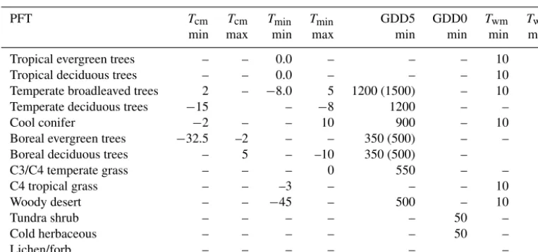
Basic input variables are monthly mean climatologies of temperature, cloud cover (sunshine) and precipitation as well as the absolute minimum temperature, the atmospheric CO2 concentration and soil physical properties such as the water holding capacity and percolation rates. These soil properties are based on global soil maps provided by the Food and Agri-culture Organisation (FAO, 1995). The model distinguishes 13 different PFTs that are defined by physiological attributes and bioclimatic tolerance limits such as heat, moisture and chilling requirements or the cold resistance of the plants (Ta-ble 1). These limits determine the area where the PFTs could exist in a given climate. Competition between the calculated PFTs is incorporated by ranking the PFTs according to their
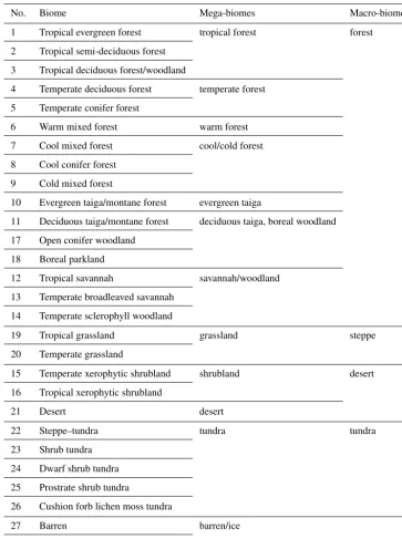
simulated relative net primary productivity (NPP), leaf area index (LAI) and the mean soil moisture (Kaplan et al., 2003). The biomes are then identified based on the dominant and second-most dominant PFTs. The original BIOME4 version includes 28 different biomes. To better track main biome shifts throughout the Holocene, we further grouped them into 12 mega-biomes (Table 2).
BIOME4 has originally been designed and calibrated to resolve global vegetation distributions under modern atmo-spheric CO2 concentrations (325 ppm). To give considera-tion to the lower atmospheric CO2level during the Holocene as well as to the biome diversity and unique environment formed in the complex topography of Asia, we slightly mod-ified and recalibrated the model. In detail, the following changes have been undertaken:
1. We implemented dependence of bioclimatic limits on the orography to better represent the vegetation in high-elevated areas such as the flanks of the Tibetan Plateau. In general, the bioclimatic limits given in the global BIOME4 model represent the horizontal biome differ-entiation (e.g. taiga and tundra, i.e. the northern line), but the limits in the vertical (e.g. the upper tree-line) differ. Limits were taken from BIOME4-TIBET (Ni and Herzschuh, 2011). We choose the ETOPO5 dataset (Data Announcement 88-MGG-02: Digital re-lief of the Surface of the Earth; NOAA, National Geo-physical Data Center, Boulder, Colorado, 1988) as orog-raphy.
Cool conifer −2 – – 10 900 – 10 –
Boreal evergreen trees −32.5 –2 – – 350 (500) – – –
Boreal deciduous trees – 5 – –10 350 (500) – –
C3/C4 temperate grass – – – 0 550 – – –
C4 tropical grass – – –3 – – – 10 –
Woody desert – – −45 – 500 – 10 –
Tundra shrub – – – – – 50 – 15
Cold herbaceous – – – – – 50 – 15
Lichen/forb – – – – – – 15
is conform with observations and operated well in test runs. In warm regions (growing degree days (GDD5) exceed 1200◦C) with less than 400 mm of rain per year, steppes are preferred. In warm regions with less than 200 mm year−1, deserts prevail (Pfadenhauser and Kloetzli, 2014).
3. We re-calibrated the model for pre-industrial CO2 con-centration (280 ppm) and the new reference climate data, the University of East Anglia Climatic Research Unit Time Series 3.10 (CRU TS3.10, University of East Anglia, 2008; Harris et al., 2014), i.e. we slightly modi-fied the LAI and NPP constraints in the PFT and biome assignment to better match the observed vegetation dis-tribution (see Fig. A1 in Appendix A). The new LAI and NPP limits are within the range of observations, but LAI and NPP measurements strongly vary and profound and comprehensive dataset do not exist for the Asian region.
The difference between the modified and original BIOME4 model can be seen in Appendix A (Fig. A2) based on the pre-industrial reference simulation and the ensemble mean simulation for the mid-Holocene (including comparison with reconstructions).
2.2 Reference simulation 0 k
As reference simulation for the modern biome distribu-tion (named pre-industrial or 0 k in the following), we forced BIOME4 with the modern monthly mean climatol-ogy (1960–2000) taken from CRU TS3.10 providing a more reliable climate background than pindustrial climate re-constructions or simulations. However, we prescribed pre-industrial atmospheric CO2 concentration (280 ppm) to be
consistent with the transient mid-Holocene to pre-industrial climate simulations and to partly come up with the fact that modern vegetation is not supposed to be in equilibrium with the fast changing atmospheric CO2 level. The differ-ences between the reference simulation using 280 ppm and a simulation prescribing 360 ppm can be seen in Appendix A (Fig. A3).
Furthermore, the CRU TS3.10 data are provided in rel-atively high spatial resolution of 0.5◦×0.5◦, resolving the climate gradients along the complex Asian orography better than the global climate model simulations.
Particu-Table 2.Biomes calculated in BIOME4 and their classification into mega-biomes and macro-biomes that are considered in this study (see Fig. 2).
No. Biome Mega-biomes Macro-biomes
1 Tropical evergreen forest tropical forest forest
2 Tropical semi-deciduous forest
3 Tropical deciduous forest/woodland
4 Temperate deciduous forest temperate forest
5 Temperate conifer forest
6 Warm mixed forest warm forest
7 Cool mixed forest cool/cold forest
8 Cool conifer forest
9 Cold mixed forest
10 Evergreen taiga/montane forest evergreen taiga
11 Deciduous taiga/montane forest deciduous taiga, boreal woodland
17 Open conifer woodland
18 Boreal parkland
12 Tropical savannah savannah/woodland
13 Temperate broadleaved savannah
14 Temperate sclerophyll woodland
19 Tropical grassland grassland steppe
20 Temperate grassland
15 Temperate xerophytic shrubland shrubland desert
16 Tropical xerophytic shrubland
21 Desert desert
22 Steppe–tundra tundra tundra
23 Shrub tundra
24 Dwarf shrub tundra
25 Prostrate shrub tundra
26 Cushion forb lichen moss tundra
27 Barren barren/ice
28 Land ice
larly the non-forest biomes, e.g. different herbs, cannot prop-erly be represented by the limited number of PFTs used in BIOME4. The model cannot distinguish biomes sharing sim-ilar PFTs under simsim-ilar bioclimatic conditions, which is par-ticularly problematic for describing different types of tundra and mountainous vegetation (Ni and Herzschuh, 2011). In addition, bioclimatic constraints are defined to characterise global vegetation and are therefore too broad to represent all regional vegetation types appropriately, even though we
adapted the climate limits and biome assignment rules. Fur-thermore, better resolved soil properties datasets are needed to improve the vegetation simulation.
com-Figure 2.Simulated biome distribution based on the University of East Anglia Climatic Research Unit Time Series 3.10 (CRU TS3.10, University of East Anglia, 2008; Harris et al., 2014) in comparison to the reference dataset (modified from Hou, 2001; Saandar and Sugita, 2004; and Stone and Schlesinger, 2003).
pensate for regions with little or no observational data enter-ing the dataset.
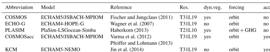
2.3 Transient climate forcing data for the Holocene To assess the Holocene vegetation changes in Asia, we drive BIOME4 with output of five different transient climate model simulations performed in a wide spectrum of fully coupled atmosphere–ocean–vegetation models. Although most of the models integrate versions of the ECHAM atmosphere model, the oceanic models are different leading to different climates in the here used simulations.
All climate models have been run into quasi-equilibrium under early- or mid-Holocene orbital conditions. After-wards, the orbital parameters (Berger, 1978) were contin-uously being changed until pre-industrial (0 k) conditions were reached. We started our analysis with the mid-Holocene time slice, i.e. 6000 years before present (henceforth referred to as 6 k). Atmospheric composition has been kept constant at pre-industrial values with CO2concentration set to 280 ppm in most models. Since the absolute minimum temperature (Tmin) was not provided by all models, we consistently cal-culatedTminfrom the mean temperature of the coldest month as described in Prentice et al. (1992). The models have been tested to capture the present-day Asian climate, in particular the Asian monsoon climate (see Dallmeyer et al., 2015). A short overview of the different climate simulations is given below and summarised in Table 3. For details, we refer to the given references.
2.3.1 COSMOS and COSMOSacc
COSMOS is the model of the Community Earth System Models network, initiated by the Max Planck Institute for Meteorology. The model consists of the atmospheric general circulation model (GCM) ECHAM5 (Roeckner et al., 2003), coupled to the land-surface and vegetation model JSBACH (Raddatz et al., 2007) and the Ocean model MPIOM (Mars-land et al., 2003), and the Ocean-Atmosphere-Sea Ice-Soil coupler (OASIS3; Valcke et al., 2003; Valcke, 2013), which enables the atmosphere and ocean to interact with each other. JSBACH includes the dynamic vegetation module of Brovkin et al. (2009). ECHAM5 ran with a spectral resolu-tion of T31L19, which corresponds to a longitudinal distance of approx. 3.75◦and 19 levels in the vertical. The MPIOM was employed at a horizontal resolution of GR30 (formal res-olution of∼3◦×3◦) with 40 vertical levels. In this set-up, two simulations have been performed, one with an acceler-ated orbit and one without acceleration. In the acceleracceler-ated simulation (COSMOSacc; Varma et al., 2012; Pfeiffer and Lohmann, 2013), the orbital forcing was accelerated by a factor of 10, so that the Holocene is represented by only 600 instead of 6000 model years. In the non-accelerated simula-tion (COSMOS; Fischer and Jungclaus, 2011), orbital forc-ing was applied on a yearly basis. Atmospheric composition was fixed to pre-industrial values in both simulations.
2.3.2 ECHO-G
Table 3.Overview on all climate simulations used as forcing for BIOME4. Given is also the model resolution (Res.), as well as whether a dynamic vegetation module has been coupled (dyn.veg.) and accelerated forcing has been used (acc.).
Abbreviation Model Reference Res. dyn.veg. forcing acc.
COSMOS ECHAM5/JSBACH-MPIOM Fischer and Jungclaus (2011) T31L19 yes orbit no
ECHO-G ECHAM4-HOPE-G Wagner et al. (2007) T31L19 no orbit no
PLASIM PlaSim-LSGocean-Simba Haberkorn (2013) T21L10 yes orbit+GHG no
COSMOSacc ECHAM5/JSBACH-MPIOM Varma et al. (2012) T31L19 yes orbit yes
Pfeiffer and Lohmann (2013)
KCM ECHAM5-NEMO Jin et al. (2014) T31L19 no orbit yes
al., 1997), which has an effective horizontal resolution of 2.8◦×2.8◦ using grid refinement in the tropical regions. In the transient simulation analysed in this study, non-accelerated orbital forcing was applied (Wagner et al., 2007). The atmospheric composition was fixed to pre-industrial level. No interactive vegetation changes were used in this model simulation; i.e. the model is run with constant pre-industrial vegetation cover.
2.3.3 KCM
The Kiel Climate Model (KCM; Park et al., 2009) consists of the atmospheric GCM ECHAM5 (Roeckner et al., 2003) coupled to the ocean/sea-ice GCM NEMO (Madec, 2006). ECHAM5 ran in the numerical resolution T31L19 corre-sponding to 3.75◦on a great circle. NEMO ran with a hor-izontal resolution of approx. 2◦×2◦ with increased merid-ional resolution of 0.5◦ close to the equator. The transient simulation analysed in this study covers the last 9500 years prescribing orbital forcing only (Jin et al., 2014). The change in orbital parameter was accelerated by a factor of 10. Green-house gas concentration was kept constant on pre-industrial values.
2.4 PLASIM
PLASIM is an atmosphere model of medium complexity (Fraedrich, 2005) and ran with a horizontal resolution of T21 (approx. 5.6◦×5.6◦on a Gaussian grid) and 10 levels in the vertical. In the simulation used for this study, PLASIM was coupled to the ocean model LSG (Maier-Reimer et al., 1993) and the vegetation module SimBA (Kleidon, 2006). The tran-sient simulation was not accelerated (Haberkorn, 2013); i.e. orbital forcing was applied on a yearly basis. In contrast to most other simulations, Holocene variations in atmospheric CO2 concentration were additionally prescribed (from Tay-lor Dome; Indermuhle et al., 1999). Atmospheric CO2 con-tent was changed from 265 to 269 ppm during mid-Holocene to pre-industrial level (280 ppm). As the forcing related to the increase in CO2 is relatively small compared to the or-bital forcing, we do not expect any substantial impact of the non-constant CO2on the results drawn in this study.
2.5 Calculation of biome distributions for the Holocene
The biome distributions were calculated for time slices throughout the last 6000 years with an interval of 500 years. We used an anomaly approach to minimise the influence of systematic biases in the climate simulations on the vegetation distributions (see Wohlfahrt et al., 2008). For this purpose, the climate model outputs have been interpolated linearly to the 0.5◦grid used in the CRU TS3.10 climate reference data. Then, the absolute differences between the monthly mean cli-matologies (long-term averages of 120 years; e.g. year 1–120 (1–12) of each model simulation for 6 k, year 501–621 (51– 62) for 5.5 k, the last 120 (12) years for 0 k) simulated for each time slice and the simulated pre-industrial climate have been added to the reference dataset. Negative values in pre-cipitation or sunshine resulting from a too large negative dif-ference of the variables between 6 and 0 k, compensating the present-day values, have been set to zero. This anomaly ap-proach has the advantage of preserving regional climate pat-tern although the complex Asian orography is not resolved in the coarse spatial resolution used in the climate simulations (Harrison et al., 1998). We are, however, aware of the simpli-fications inherent to this approach in interpolating coarsely resolved GCM output (resolution approx. 3.75◦and coarser) onto higher target grids (here 0.5◦) without taking into ac-count potentially important factors that lead to local varia-tions in climate, such as changes in variability and feedbacks from the local to the meso and large scale. Considering the general character of our study this approach should, how-ever, compensate for some of the GCM-related shortcom-ings related to orography and according processes. Atmo-spheric CO2 concentration has been fixed to pre-industrial value (280 ppm) in all biome simulations.
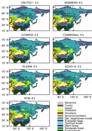
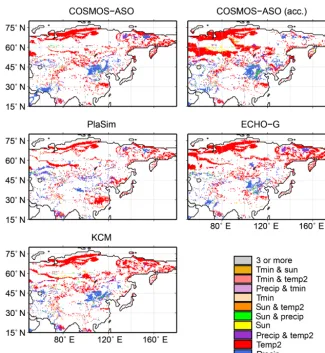
Figure 3.Simulated biome distributions for the modern climate (CRU TS3.10 0 k) and for the mid-Holocene time slice (6 k) based on the ensemble mean climate (ENSMEAN) and the different climate model simulations. In the plot of the ensemble mean, the two key regions of biome changes are marked (red boxes): the taiga–tundra transition zone in north-central Siberia (66–120◦E, 60–80◦N) and the forest– steppe–desert transition zone in north-central China (95–125◦E, 32–52◦N).
of the CRU TS3.10 dataset, as well as the simulated mid-Holocene precipitation.
To facilitate the discussion of the results, the biome simu-lations are named after the climate model simulation serving as input for the BIOME4 model; e.g. the biome simulation forced with the climate calculated in COSMOS is referred to COSMOS in the following.
2.6 Pollen-based biome reconstruction for key areas of vegetation change
compari-Figure 4.Simulated percentages of land area (%) for each biome at pre-industrial (hatched) based on CRU TS3.10 and mid-Holocene (fully shaded) averaged over the entire region considered here (60–180◦E, 15–80◦N) and averaged over all simulations, including the ensemble standard deviation (error bars).
son, representative, high quality (with respect to dating and the data) pollen records covering the last 6000 years have been chosen. For the taiga–tundra transition zone, a record from a small lake located on the southern Taymyr Peninsula (technical name: 13-CH-12; Klemm et al., 2016) is used that is in line with the vegetation trend seen at other records lo-cated at the Siberian treeline (Pisaric et al., 2000; MacDonald et al., 2000; Bigelow et al., 2003). The biome change in the forest–steppe transition zone is reflected by the record from Lake Daihai in Inner Mongolia (China; 40.5◦N, 112.5◦E; 1225 m a.s.l.; Xu et al., 2010) that is in line with other records in north-central China (Zhao et al., 2009, and references therein). To better compare the simulated biome distribution, these records were biomised in accordance with the BIOME4 biome classification. We applied the standard biomisation procedure to assign pollen taxa first to PFTs and in a sec-ond step PFTs to biomes (Prentice et al., 1996) through a global classification system that was specified for East Asia in Ni et al. (2014), but excluding anthropogenic PFTs. Fi-nally, for each pollen spectrum in a record an affinity score for each biome is calculated. It is assumed that the biome with the highest score dominates in the pollen-source area of the lake, while a relatively lower score indicates less occur-rence of a biome in the area. Accordingly, only the dominant biome types and the trends of different biomes but not their absolute coverage can be compared to model-based results. Please notice that the pollen reconstructions are dated in cal-ibrated years before present, i.e. before the year 1950 AD (ca ka BP), and thus the time step 0 cal. ka BP is not identi-cal with the time slice “0 k” used in the modelling result (i.e. a mean of 120 years).
3 Results
3.1 Simulated mid-Holocene biome distributions
Figure 3 shows the mid-Holocene biome distribution corre-sponding to the different climate simulations. Overall, the vegetation change is small and similar for all models. The main biome shifts occur in the high northern latitudes and in the transition zone of desert, steppe and forests in East Asia (95–125◦E, 32–52◦N).
Compared with the pre-industrial situation, deciduous taiga and boreal woodland further penetrate northward dur-ing mid-Holocene and the boreal tree line is shifted to the north by about 3–5◦in the ensemble mean (for simplification,
only◦is used for geographical distances given in degrees of
latitude or longitude in the following). This shift ranges from approximately 1–2◦in PLASIM to 4–6◦in COSMOSacc.
The desert–steppe margin in East Asia is located further west by approx. 4◦in the ensemble mean, substantially re-ducing the desert area in East Asia at mid-Holocene. The maximum response is found in COSMOSacc (approx. 9◦), while the weakest signal is shown by PLASIM (approx. 1◦). The cool/cold forest and taiga biomes extend further north-westward into the pre-industrial East Asian steppe at 6 k (ap-prox. 2◦ in ensemble mean). The largest change occurs in COSMOS (3–4◦). The climate change in PLASIM is too weak to induce a shift of the forest–steppe border in the southern part of the transition zone, north of 41◦the steppe expands to the east.
Figure 5.Factors causing a change in biome distribution as simulated by BIOME4 forced with climate data from different climate model simulations, i.e. precipitation (precip), near-surface air temperature (temp2), sunshine/cloudiness (sun) or absolute minimum temperature (Tmin).
as large as the mean change. Evergreen (6 %) and deciduous (27 %) taiga strongly expand at the expense of tundra that ex-perienced a reduction in area by 35 % during mid-Holocene. The total change of shrubland and savannah/woodland is small. The area of grassland is increased by approximately 28 % at mid-Holocene compared to the modern distribution. The desert fraction is reduced by 14 %.
3.2 Climate factors determining the vegetation change in eastern Asia
The Holocene changes in bioclimate are discussed in Ap-pendix B (Fig. B1). To assess the climate variables be-ing responsible for the biome shifts in the model since the mid-Holocene, climate variables of the pre-industrial input dataset are gradually replaced by the respective variable of the simulated mid-Holocene climate. The results of this sensitivity study are shown in Fig. 5. As expected, most biome shifts between mid-Holocene and pre-industrial can be related to changes in temperature or precipitation. The
prolongation of the warm season, associated with the gen-eral warmer summer climate in the northern latitudes (see Fig. B1), leads to the northward expansion of boreal forest. The biome shifts at the forest–steppe–desert transition in East Asia can already be induced by the mid-Holocene to pre-industrial precipitation change. The cloud cover (sunshine) plays a minor role and is mainly relevant in the differentia-tion of cold/cool forest and taiga (e.g. in COSMOSacc). The absolute minimum temperature has mainly an impact in the tropical region, where the decreased cold season tempera-ture during the mid-Holocene leads, for example, to a slight southward shift of the tropical forest belt.
3.3 Transient biome shifts at the forest–steppe–desert transition zone in north-central China
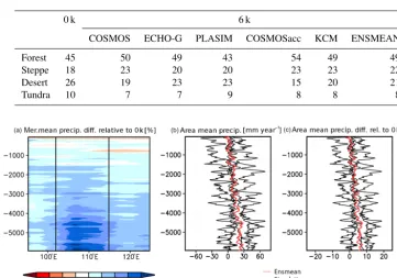
Table 4.Mean coverage of macro-biomes (absolute %) in the forest–steppe–desert transition zone (95–125◦E, 32–52◦N) according to the reference simulation (0 k) and the different simulations using mid-Holocene climate.
0 k 6 k
COSMOS ECHO-G PLASIM COSMOSacc KCM ENSMEAN
Forest 45 50 49 43 54 49 49
Steppe 18 23 20 20 23 23 22
Desert 26 19 23 23 15 20 21
Tundra 10 7 7 9 8 8 8
Figure 6.Mid-Holocene to pre-industrial precipitation change in the desert–steppe–forest transition zone (95–125◦E, 32–52◦N; land only). (a)Hovmoeller diagram showing the ensemble mean of the meridional mean (32–52◦N) relative difference in annual precipitation (%) compared to pre-industrial; the black lines mark the regions with strongest signal.(b)Area mean precipitation (mm year−1) averaged over all simulations (red) and for each single simulation (black).(c)Area mean relative change in precipitation compared to pre-industrial (%).
respectively). Tundra biomes cover only 10 % of the region (Table 4). Averaged over the area, the pre-industrial desert– steppe margin is located at 113◦E and the forest–steppe mar-gin at 120◦E (Table 5). This distribution has changed in the last 6000 years, probably due to differences in precipitation (see Fig. 5). Figure 6 shows the simulated area mean and the meridional mean change in annual precipitation since the mid-Holocene relative to the modern precipitation (ensemble mean). Precipitation is increased by approx. 8 % on average and even by more than 15 % in a broad region directly east of the pre-industrial desert–steppe margin (approx. 113◦E in the mean). In this region, rainfall stays on a relatively high level until 4.2 k and eventually starts to decrease gradually, reaching modern climate conditions around 1.5 k. This in-duces a reduction of the desert and a shift in the mean desert– steppe border. During the mid-Holocene, the area in the tran-sition zone covered by desert biomes is declined by approx. 21 % in the ensemble mean, ranging from a decreased frac-tion by 42 % at mid-Holocene in one simulafrac-tion and a simi-lar desert fraction as in modern climate in another simulation (Fig. 7).
Averaged over all simulations, the mean desert border is located at 108◦E during the mid-Holocene, staying relatively
constant until 4.5 k. Afterwards, a shift of about 100 km to the east within 500 years occurs. The desert border stays
rel-atively constant again until 2 k and then moves gradually to its modern position. This gradual decline is interrupted by a period with strongly increased desert fraction compared to the millennia before at 1.5 k.
On a regional scale, most simulations reveal a substan-tially reduced desert fraction in large parts of the transition zone. During the entire period, the desert fraction is substan-tially reduced in a broad band between 102 and 115◦E.
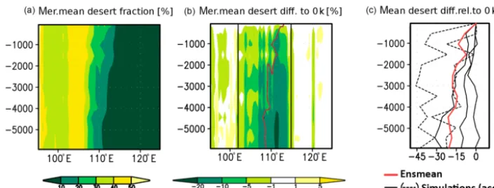
Figure 7.Mid-Holocene to pre-industrial desert biome change in the desert–steppe–forest transition zone (95–125◦E, 32–52◦N; land only). (a)Hovmoeller diagram showing the ensemble mean of the meridional mean (32–52◦N) desert fraction (% fraction of area).(b)Hovmoeller diagram showing the absolute change in meridional mean desert fraction (%) compared to pre-industrial as ensemble mean. The red line marks the steppe border (here ad hoc defined as the isoline of 20 % desert fraction) and the black lines mark the regions with strongest precipitation change (cf. Fig. 6).(c)Area mean relative change in desert fraction compared to pre-industrial averaged over all simulations (red) and for each single simulation (black). The dashed line displays the accelerated simulations.
Figure 8.Same as Fig. 7 but for forest fraction.(b)Red line displays the steppe–forest margin (here ad hoc defined as isoline of 80 % forest fraction).
the last 6000 years (Figs. 8 and C2 in Appendix C). In most simulations, the forest fraction is increased in large parts of the region during the mid-Holocene, but they also suggest several periods with less forest than in other periods, at least on a local scale, e.g. between 3 and 3.5 k and around 1.5 k in the ensemble mean. The simulations based on the acceler-ated climate models reveal a much stronger response to the climate forcing than the other simulations.
Averaged over all simulations, the area in the transition zone covered by forest biomes is increased by approx. 8 % during the mid-Holocene compared to the modern frac-tion (Fig. 8). The maximum forest extent during the last 6000 years is reached at 5 and 2.5 k with an increase in forest fraction by 12 % compared to the modern distribution. How-ever, the relatively small expansion of forest during the mid-Holocene is deceptive, because BIOME4 tends to replace taiga and cold forest with grass at the northern part of the transition zone and east of the Tibetan Plateau (100–110◦E) due to higher temperatures at 6 k. This tendency becomes
particularly clear when looking at the simulated meridional mean change in forest cover since the mid-Holocene (Fig. 8). In all simulations, forest cover is suggested to be decreased in the region between 103–110◦E at 6 k. Averaged over all simulations, this period of reduced forest areas lasts until 4 k, ranging from 5 k in COSMOSacc to 0.5 k in ECHO-G.
In the region around 100◦E, all simulations show an in-crease of the forest fraction (10 % in the ensemble mean), which can mainly be attributed to an expansion of taiga on the Altai Mountains and on the Tibetan Plateau. The forest cover gradually decreases and reaches modern conditions at 2 k in most simulations.
Table 5.Summary of the mean positions of the desert–steppe (20 % isoline of desert fraction), forest–steppe (80 % isoline of wood fraction) and taiga–tundra border (20 % isoline of tundra fraction) in the different simulations during pre-industrial and mid-Holocene.
Border 0 k 6 k
COSMOS ECHO-G PLASIM COSMOSacc KCM ENSMEAN
Desert–steppe 113◦E 107◦E 110◦E 112◦E 104◦E 107◦E 108◦E
Forest–steppe 120◦E 117◦E 119◦E 124◦E 119◦E 117.5◦E 118◦E
Taiga–tundra 67.5◦N 73.5◦N 73.5◦N 69◦N 73.5◦N 71◦N 71.5–73◦N
Figure 9.Mid-Holocene to pre-industrial 2 m air temperature change in the north-central Siberian taiga–tundra margin (66–120◦E, 60– 80◦N; land only).(a)Hovmoeller diagram showing the ensemble mean of the zonal mean absolute difference in annual mean near-surface air temperature (K) compared to pre-industrial;(b)area mean annual mean 2 m air temperature (K) averaged over all simulation (red) and for the individual simulations (black);(c)area mean absolute difference in annual mean near-surface air temperature compared to pre-industrial averaged over all simulation (red) and for each simulation (black).
more than 20 % and a westward shifted forest–steppe border by approx. 3◦at 6 k. However, PLASIM suggests a relatively
weak forest response to the Holocene climate forcing. The forest fraction is increased between 113 and 118◦E from 6 to 1 k, but decreased eastward of 118◦E by more than 10 % dur-ing the entire period, actually resultdur-ing in an eastward shifted mean forest–steppe border.
3.4 Transient biome shift in the north-central Siberian taiga–tundra transition zone
According to the pre-industrial biome simulation, the north-central Siberian taiga–tundra transition zone (66–120◦E, 60– 80◦N) consists of 27 % tundra and 73 % taiga (Table 6). The mean taiga–tundra border is located at 67.5◦N (Table 5). The vegetation in the high northern latitudes is particularly sensitive to changes in temperature (see Fig. 5). In the area mean and averaged over all simulations, the temperature is increased by approx. 1 K during the mid-Holocene, ranging from 1.9 K in ECHO-G to 0 K in PLASIM (Fig. 9). The cli-mate in the northern parts of the region, i.e. north of ca. 71◦N, stays relatively warm until 4.5 k, showing increased temperatures by more than 0.75 K in the ensemble mean. This warm period is interrupted several times by slightly colder periods. The southern part stays warm (>0.5 K)
un-til 2.5 k. Afterwards, the climate in the north-central taiga– tundra margin is similar to pre-industrial. These changes in temperature lead to an increase in forest cover and a north-ward shift of the taiga belt.
All simulations show a substantially increased extent of taiga forest during the mid-Holocene and in the following millennia (Figs. 10 and C3 in Appendix C). In the ensemble mean, the mean taiga border is located at 71.5◦N at 6 k with some extension to 73◦N. In large parts of the area, the tun-dra fraction is reduced by more than 25 % at mid-Holocene, directly at the taiga border by even more than 50 % (absolute values). The areal mean tundra fraction is decreased by 64 % at 6 k relative to the 0 k extent (Fig. 10).
Averaged over all simulation, the taiga retreats relatively fast southward until 4 k (back to 68.5◦N) and then moves gradually and slowly back to the modern position. Neverthe-less, the north-central Siberian taiga–tundra transition zone is characterised by a substantially increased taiga fraction dur-ing most of the period, staydur-ing on a high level until 1.5 k.
Figure 10.Mid-Holocene to pre-industrial tundra fraction change in the north-central Siberian taiga–tundra margin (66–120◦E, 60–80◦N; land only).(a)Hovmoeller diagram showing the ensemble mean of the zonal mean tundra fraction (% fraction of area);(b)same as(a)but for the absolute change in zonal mean tundra fraction (%) compared to pre-industrial as ensemble mean. The red line marks the taiga border (here ad hoc defined as the isoline of 20 % tundra fraction).(c)Area mean relative change in tundra fraction compared to pre-industrial averaged over all simulation (red) and for each simulation (black, dashed line: accelerated simulations).
tundra fraction north of 70◦N at 1.5 k. PLASIM reveals the weakest signal with a reduction by 48 % and a shift of the taiga–tundra margin by only 1.5◦during the Holocene. In-terestingly, COSMOS reveals a period with substantially re-duced taiga fraction around 4 k (up to 25 %), resulting in a southward retreat of the taiga border to 68◦N.
3.5 Pollen-based biome reconstruction for the
forest–steppe transition and the taiga–tundra zones Figure 11 shows the reconstructed biome change based on two pollen records representing the vegetation change in the key regions experiencing the most pronounced changes in the biome simulations, i.e. the forest–steppe–desert transi-tion zone in north-central China (represented by Lake Daihai record) and the taiga–tundra transition zone in north-central Siberia (represented by the record on the southern Taymyr Peninsula). Also shown are the simulated biome changes in the surroundings of these sites. In contrast to the simulated biome change, the reconstructions do not show an absolute change in biome coverage. They depict the trend only semi-qualitatively and can be interpreted as change in the simi-larity of reconstructed pollen taxa composition to a certain biome.
According to the biome reconstructions, cool-mixed forests slightly dominate over steppes and temperate xero-phytic shrublands at Lake Daihai in the forest–steppe–desert
transition zone during mid-Holocene. After 5.1 cal ka BP, biome composition is characterised by a dominance of steppes and temperate xerophytic shrublands (assigned to desert in the BIOME4 macro-biome classification). The overall increasing trend in steppe and deserts and decreas-ing trend in forest is interrupted by periods with substantially raised forest biome similarity around 3.7 and 1.6 cal ka BP. Forest trend is reversing in the last 400 years.
4 Discussion
4.1 Differences in biome simulations originating from weaknesses in simulated climate
One aim of this study is the representation of a range of possi-ble biome changes in Asia during the last 6000 years. For this purpose, we forced BIOME4 with simulated climate anoma-lies from various global climate models. The outcome of this analysis and its reliability depends directly on the capability of the models to simulate the mid-Holocene to pre-industrial climate change. Biases in the models and differences in the simulated climate between the individual models lead to er-rors and differences in the simulated biome distributions. Re-cent studies revealed that climate models have large deficits in representing the present-day mean precipitation distribu-tion and seasonal cycle of the Asian monsoon system (Kang et al., 2002; Zhou et al., 2009; Boo et al., 2011) that affect large parts of the area under consideration in this study. Tem-perature distributions are generally better captured by the models.
A detailed assessment of the performance of the models used in this study with respect to the Asian monsoon pre-cipitation distribution has been conducted in Dallmeyer et al. (2015). In general, the models reveal similar biases re-garding the precipitation pattern, but the amplitude diverges. All of the models overestimate the present-day annual pre-cipitation in central and north-eastern China. In the East Asian monsoon transition zone, simulated precipitation ex-ceeds the observations by up to 900 mm year−1 in the en-semble mean. As we use climate anomalies between the dif-ferent time slices and pre-industrial and add them to obser-vational data, this bias in precipitation should not affect the simulated biome distributions. The models respond very dif-ferently to the insolation forcing, revealing large differences in model sensitivity that have an impact on the simulated biome distribution. PLASIM generally shows a rather weak response. The PLASIM simulation ran at coarser resolution than the other simulations. In the pre-industrial control run, the Asian monsoon strength is underestimated by the model (see Dallmeyer et al., 2015) and thus the dynamic of the monsoons might not be represented correctly. The acceler-ated simulations reveal a rather strong response and exhibit large variability. The latter is at least partly due to the method of averaging the climate forcing data. We took the climatol-ogy of 120 calendar years as representative of the climate at the individual time slices. These are 120 model years in the non-accelerated simulations, but only 12 years in the accel-erated simulations.
In general, the coarse resolution of the models may lead to uncertainties in the biome simulations. Local (sub-grid scale) climate and vegetation changes cannot be represented in the simulations, but they may be recorded in reconstruc-tions showing mostly the vegetation change in, for example, the catchment area of the lakes. The coarse resolution may,
thus, lead to artefacts in the shift of vegetation zones; e.g. if the precipitation increases in one grid box column at the desert–steppe margin, the steppe also shifts by one grid box column since sub-grid changes are not resolved.
Furthermore, different spatial resolutions lead to differ-ent represdiffer-entations of the elevation in the climate models, which may have an impact on the climate change during the Holocene, particularly in high-elevated regions. As we use the anomaly method to calculate the biome distribution, the elevation – or more precisely – the climate gradients result-ing from the elevation are preserved from the CRU reference climate. Implicit in this widely used downscaling approach is the assumption that the temperature lapse rate does not change with climate. This is a fair assumption, if not drasti-cally different climate states (e.g. glacial vs. interglacial cli-mate) are considered.
At least partly, the discrepancies in simulated climate may be related to the differences in interactive model components used in the climate model; i.e. some models include dynamic vegetation some do not. Previous modelling studies indicate that land-surface feedbacks with the atmosphere could have enhanced the Holocene precipitation change induced by or-bital forcing in the Asian monsoon region (e.g. Wang, 1999; Texier et al., 2000; Diffenbaugh and Sloan, 2002; Li et al., 2009). To test the influence of dynamic vegetation on the simulated Asian climate, sensitivity simulations have to be undertaken. An appropriate set of experiments only exists in the COSMOS set-up (see Dallmeyer et al., 2010). Accord-ing to these simulations, interactive vegetation has a negligi-ble effect on the mid-Holocene to pre-industrial precipitation change in the desert–steppe–forest transition zone. Vegeta-tion feedbacks contribute to the warmer mid-Holocene cli-mate in the high northern latitudes, but the interactive ocean has a much stronger impact on the climate change. There-fore, the lack of interactive vegetation in KCM and ECHO-G may partly lead to biases in simulated climate change, but we do not expect an effect of this on the general results of this study.
4.2 Comparison with pollen-based biome reconstructions
mod-Figure 11.Reconstructed biome change at two representative key sites:(a)Lake Daihai (40.5◦N, 112.5◦E; Xu et al., 2009) for the forest– steppe–desert transition zone and(b)a small lake on the southern Taymyr Peninsula (13-CH-12; 72.4◦N, 102.29◦E; Klemm et al., 2016) for the taiga–tundra margin. The reconstructions are given in arbitrary units and show the dominant biome at a certain time and the trend qualitatively (i.e. less or more dominant than other biomes). Shown are also the simulated biome change in the surrounding of both sites, i.e. 110–114◦E, 38–42◦N for Lake Daihai and 106–110◦E, 69–73◦N for the southern Taymyr record. The latter region had to be adjusted to the modern taiga–tundra margin that is shifted northward in the modern biome simulation due to an overestimation of forest cover in the boreal region. For comparison, the nearest grid box around the lake showing tundra vegetation in modern climate has been taken. The reconstructions are given in fractional coverage per area (%).
elling is often described in the form of few PFTs (within cou-pled dynamic vegetation models) or biomes (within diagnos-tic vegetation models).
Therefore, we translate representative records of recon-structed plant taxa into biomes that are in accordance with the biome classifications used in BIOME4 (Fig. 11), i.e. the Lake Daihai record (forest–steppe–desert transition zone) and the 13-CH-12 record (taiga–tundra transition zone). The Lake Daihai biome reconstruction, indicating a dominance of cool mixed forests during the mid-Holocene, reflects the expansion of pine forests in the uplands as depicted by the high Pinus-pollen percentage in the pollen spectra (Xu et al., 2010). However, the low land most probably was covered by steppe vegetation throughout the Holocene. This general trend of a mid-Holocene maximum is known from further sites in north-central China (e.g. Shi and Song, 2003; Jiang et al., 2006; Zhao et al., 2009), while sites on the Tibetan Plateau rather indicate an early-to-early-mid-Holocene for-est and vegetation maximum (e.g. van Campo et al., 1996;
Shen et al., 2005; Zhao et al., 2009). At present day, steppe is the dominant biome in the Lake Daihai region, while forests are substantially reduced. Furthermore, taxa composition has a high resemblance with temperate xerophytic shrublands, probably reflecting an increase in shrubland and desert vege-tation in this region. Human interference cannot be excluded at this site (see Xiao et al., 2004) but may have affected vege-tation change since the mid-Holocene rather locally. In east-ern and central Asia, overall climate is assumed to be the major driver of forest decline (e.g. Wang et al., 2010; Cao et al., 2015; Tian et al., 2016).
forest and taiga biomes into the pre-industrial East Asian steppe. The desert-to-steppe border (including desert and xe-rophytic shrubland biomes) is even shifted approx. 450 km to the west. However, the models reveal strong discrepan-cies among each other with respect to the vegetation distribu-tion and temporal change. Regarding the vegetadistribu-tion change around Lake Daihai (in the model: 110–114◦E, 38–42◦N), the models mostly agree with the biome reconstruction on the long term, showing a decrease of cool/cold forest and an increase of grassland and shrublands since the mid-Holocene in the ensemble mean (see Fig. 11). They even reveal short-time recovering of the forest biome at certain phases, e.g. around 5, 2 and 1 k. The timing of these phases deviates from the reconstruction, but, as mentioned before, the spread in the simulated vegetation change between the different climate models is large. Furthermore, the catchment area of Lake Daihai is not exactly definable and does most probably not coincide with the region chosen in the model. The models re-veal regionally strong differences in the temporal forest and desert change within the forest–steppe–desert transition zone that may not be captured by the reconstructions. And last but not least, short-term (multi-centennial) variability may not be resolved in the biome simulations that have been run with coarse temporal resolution (time steps of 500 years).
The reconstructed Holocene increase of tundra and de-crease of taiga shown in the Taymyr Peninsula record from north-central Siberia is in agreement with other Holocene records from northern Siberian treeline areas (e.g. MacDon-ald et al., 2000; Herzschuh et al., 2013). It reflects the south-ward retreat of larches that coincide with the southsouth-ward shift in the boreal treeline since the mid-Holocene due to cooler climate at 0 k.
While the deciduous taiga biome reveals a clear domi-nance during mid-Holocene around lake 13-CH-12, tundra covers the landscape at present day. This is not in line with the biome simulations for pre-industrial (based on the CRU-climate dataset), showing deciduous taiga and boreal wood-lands in the region around the lake. This difference probably results from the non-equilibrium of the regional vegetation with the fast warming climate in the Arctic region. Thus, tree coverage is overestimated by the model, since temperature is the limiting factor for tree growth in this region. Furthermore, only few meteorological stations exist in northern Siberia. This fact may lead to larger uncertainties in the CRU dataset for northern Siberia compared to other regions.
Due to the overestimation of tree coverage around the lake by the biome model, we chose a corresponding region at the taiga–tundra border for comparison with the reconstructed biome trends (106–110◦E, 69–73◦N).
In general, the biome simulations are in line with the gen-eral view of reconstructed Holocene vegetation change at the boreal treeline and the record from the Taymyr Peninsula. The taiga and boreal woodlands were expanded northward during mid-Holocene, shifting the boreal treeline by approx. 4◦ to the north. The simulated biome change at the site is
large. Vegetation switches from coverage by 100 % of taiga during the mid-Holocene to coverage by 80.5 % tundra for pre-industrial. Similar to the reconstructions, the simulations also reveal periods with substantially increased tundra, i.e. at 4 and at 1 k.
5 Summary
To get a systematic overview on the Holocene vegetation change in Asia, the terrestrial biosphere model BIOME4 has been forced with climate output of five different transient simulations performed with coupled atmosphere–ocean(– vegetation) models. The differences in biome distribution be-tween the mid-Holocene and pre-industrial (potential vegeta-tion) as well as the temporal change in Holocene vegetation have been analysed.
The model results reveal only weak biome changes in Asia during the last 6000 years. Main changes concentrate on the high northern latitudes and the transition zone from the moist East Asian summer monsoon to the dry westerly winds. In the high northern latitudes the northern treeline shifts northward due to an expansion of taiga during the mid-Holocene. The vegetation in the monsoon–westerlies transi-tion area consists of desert, grassland and forest belts, whose margins shift in time. In the majority of cases, the models agree regarding the pattern of biome shift, but the amplitude of change strongly depends on the climate forcing, i.e. the different climate models.
According to BIOME4, the vegetation changes in the forest–steppe–desert transition zone (95–125◦E, 32–52◦N)
are mainly influenced by changes in precipitation. The higher moisture levels in the mid-Holocene lead to a decreased desert fraction by approx. 20 % and a westward shift of the desert–steppe boundary by approx. 500 km in the ensemble mean, ranging from 100 to 1000 km in the different simula-tions. The expansion of desert during the Holocene back to modern distribution is not uniform and varies spatially. De-pending on the climate forcing and the longitudinal position, the general trend of declining vegetation is interspersed with periods of substantially increased or decreased desert frac-tion.
Forests are increased by approx. 8 % during the mid-Holocene, penetrating into the steppe and desert regions from two sides. On the one hand, the increased precipitation at 6 k leads to a westward shifted forest–steppe boundary in east China by 2◦, ranging from 0 to 4◦ in the different
mid-approx. 400 km in the ensemble mean. From 6 to 4 k, the taiga retreats relatively fast, afterwards slowly and gradually. Some individual simulations reveal high temporal variability of tundra fraction. The biome simulations agree with vegeta-tion reconstrucvegeta-tions, but the taiga coverage is overestimated by the model, probably due to a non-equilibrium of the north-ern Siberian vegetation to the fast warming climate. One rea-son explaining the non-linear retreat of the taiga relates to the non-linear decline in northern hemispheric summer inso-lation in the course of the mid-to-late Holocene. This non-linear decline might further have been amplified by internal climate feedbacks, for instance related to the expansion and persistence of Arctic sea ice during summer.
Besides the general conclusions based on the model results one also should account for uncertainties that are included in the present results: most models used have a quite coarse hor-izontal resolution of several hundreds of kilometres – there-fore changes in the longitudinal and latitudinal spatial extent of certain biomes should show at least this order of magni-tude to allow a robust conclusion. More pollen records are needed to evaluate the simulated results, particularly in the desert–steppe transition zone.
Second and related to the last point is the aforementioned partly unrealistic representation and simulation of precipita-tion in the models. To overcome this problem one needs to carry out a regionalization of the GCM output by means of statistical and/or dynamical downscaling to yield a better ba-sis for the BIOME4 model in terms of hydrological changes or, even better, run global climate models with higher hori-zontal resolution. This methodological step is, however, be-yond the scope of this study; results that are based on thermal changes in the course of the Holocene can be expected to be more realistically simulated by the GCMs.
since the mid-Holocene, this study identifies two main re-gions with strong vegetation changes, i.e. the desert–steppe– forest transition zone related to the East Asian monsoon mar-gin and the taiga–tundra transition zone in northern Siberia. Both represent transition zones between forested and non-forested biomes. Particularly the East Asian monsoon mar-gin has hitherto been poorly documented in reconstruction. The strong spread of the simulated Holocene biome distribu-tions shows that the vegetation in these regions is very sen-sitive to variations in climate, i.e. to precipitation changes in central Asia and to temperature change in northern Siberia. Accordingly, these areas can be expected to react strongest to ongoing climate change.
7 Data availability
Appendix A: Additional figures showing the modifications of the BIOME4 model
Appendix A provides three figures which highlight the differ-ences in the BIOME-4 model as a result of our modifications.
Figure A2.Biome distributions for the modern climate (CRU TS3.10 0 k) simulated in the modified BIOME4 version (new model) and the original BIOME4 model (old model), modern biome distribution based on the reference dataset (modified from Hou, 2001; Saandar and Sugita, 2004; and Stone and Schlesinger, 2003) and biome distribution for the mid-Holocene time slice (6 k) based on the ensemble mean climate, using the modified model version and the original model. In the 6 k plots, the reconstructed biome distribution (from BIOME6000 project, http://www.bridge.bris.ac.uk/resources/Databases/BIOMES_data; Prentice et al., 2000; Harrison et al., 2001; Bigelow et al., 2003) is additionally shown for model validation (dots).
Appendix B: Bioclimatic changes
Since the simulated vegetation distributions strongly depend on the given bioclimatic conditions, we additionally identify marked changes in bioclimate between mid-Holocene and pre-industrial. Figure B1a shows the modern pattern of dif-ferent bioclimate variables that determine the biome distri-bution in Asia based on the CRU TS3.10 dataset (see Ta-ble 1). To express the moisture limitation in the semi-arid and arid regions of Asia, the annual mean precipitation and the Taylor–Priestley coefficient (α) are additionally provided. Figure B1b presents the ensemble mean difference in these bioclimatic variables between mid-Holocene (6 k) and mod-ern climate (0 k). During mid-Holocene, the annual mean near-surface air temperature is increased by up to 1.2 K in the high northern latitudes and subtropics and decreased by up to 1.9 K in the tropics, attenuating the zonal temperature contrast. This temperature change is accompanied by an in-crease in growing degree days (GDD5) north of 30◦N that is particularly pronounced in the region around the Hami and Turpan depression (up to 240◦C) and in western Siberia (up to 220◦C). South of 30◦N, growing degree days are reduced by up to 650◦C. The mean near-surface temperature during
Figure B1. Simulated bioclimate, i.e. annual mean near-surface air temperature (am. temp2), mean near-surface air temperature of the warmest month (Twm) and of the coldest month (Tcm), growing degree days on a basis of 5◦(GDD5), Taylor–Priestley coefficient of annual actual to equilibrium evapotranspiration (α) as calculated in Prentice et al. (1992) and the annual mean precipitation (am. precip),(a)based on modern climatology (CRU TS3.10) and(b)difference of the ensemble mean bioclimate at mid-Holocene and the modern climatology (6–0 k). Temperature and GDD5 are given in◦C; precipitation is given in mm year−1.
the warmest month is higher in the entire Asian region aside from India and parts of the Indochina peninsula. The max-imum warming occurs on the Tian Shan mountain range with a temperature increase by up to 3.2 K in the ensem-ble mean. The temperature of the coldest month (Tcm) is strongly increased in East Siberia by up to 1.8 K during mid-Holocene. In the other regions,Tcmis markedly lower at 6 k with anomalies reaching up to 2.7 K in India, corresponding to the decreased winter insolation during mid-Holocene.
stays relatively constant until 4.5 k. Afterwards, the desert border gradually moves eastward to its pre-industrial posi-tion, accompanying a general increase in the desert fraction that starts first in the western part (around 108◦E at ca. 4.5 k) and finally in the eastern part of the transition zone (starting at 3 k around 111◦E and at 2 k around 113◦E). However, the expansion of the desert is longitudinally not uniform: Areas around 102 and 113◦E show a relatively high degree of veg-etation cover until 0.5 k, periods with increased desert frac-tion that partly even exceeds the pre-industrial fracfrac-tion in-terrupt the periods showing higher vegetation cover between 108 and 110◦E.
Figure C1.Mid-Holocene to pre-industrial desert biome change in the desert–steppe–forest transition zone (95–125◦E, 32–52◦N; land only). Hovmoeller diagrams showing the absolute change in meridional mean desert fraction (%) compared to pre-industrial as ensemble mean and for the individual simulations. The grey lines mark the steppe border (here ad hoc defined as the isoline of 20 % desert fraction); the black lines mark the regions with strongest precipitation change (cf. Fig. 6).
Figure C2.Same as Fig. C1 but for forest fraction in the desert–steppe–forest transition zone. The grey lines display the steppe–forest margin (here ad hoc defined as isoline of 80 % forest fraction).
In contrast, the change in biome distribution based on the two accelerated simulations, i.e. COSMOSacc and KCM, shows a strong variability. The generally increased vegeta-tion cover during the Holocene compared to pre-industrial is interrupted by several periods with substantially reduced vegetation. The most prominent event occurs around 1.5 k. Similar as for ECHO-G, KCM suggests less vegetation in parts of the transition zone during the last 500 years. BIOME4 shows the strongest response using COSMOSacc as climate forcing. The desert fraction is decreased by more than 20 % in large parts of the region from 6 to 2 k and the mean desert border is shifted to 104◦E at 6 k.
Figure C2 shows the meridional mean change in forest fraction in the desert–steppe–forest transition zone for the in-dividual simulations. Directly west of the modern mean for-est border (120◦E), COSMOS and KCM reveal the strongest change with an increase of forest fraction by more than 20 % and a westward shift in the forest–steppe border by approx. 3◦. PLASIM suggests a weak change in forest coverage since
the mid-Holocene. The forest fraction is increased between 113 and 118◦E from 6 to 1 k, but decreased westward of 118◦E by more than 10 % during the entire period, actually resulting in an eastward shift of the mean forest–steppe bor-der.
ECHO-G and PLASIM suggest slightly less forest area compared to the modern distribution in nearly the entire region during the last 1000 years, while KCM and COS-MOSacc still show enhanced forest cover but with a strong decreasing trend during this period. The simulations
ECHO-G, KCM and COSMOSacc are characterised by strong vari-ability revealing several periods with substantially reduced forest fraction (e.g. 4 and 1.5 k in ECHO-G, 3.5 k in COS-MOSacc, 3 and 1.5 k in KCM). The maximum forest extent in the simulations based on the accelerated climate models is not reached during the mid-Holocene but at 5 and 4 k in COS-MOSacc and 4.5, 2 and 1 k in KCM, showing an increased forest fraction by more than 30 and 20 % during these peri-ods, respectively.
Figure C3 shows the zonal mean change in tundra frac-tion in the north-central Siberian taiga–tundra transifrac-tion zone since the mid-Holocene for all simulations.
According to COSMOS, the tundra fraction is decreased by more than 25 % in large parts of the north-central Siberian taiga–tundra transition zone during mid-Holocene. Directly at the mean taiga border, the tundra area is reduced by more than 50 %. This leads to a shift of the mean taiga border to 73.5◦N at 6 k compared to 67.5◦N at pre-industrial.
COS-MOS reveals a period with substantially enhanced tundra fraction around 4 k (up to 25 %), resulting in a southward retreat of the taiga border to 68◦N. The last 1000 years are characterised by slightly less taiga compared to pre-industrial. ECHO-G shows a similar signal but also reveals an uninterrupted and rather gradual retreat of the taiga dur-ing the Holocene.
Figure C3.Same as Fig. C1 but for the tundra fraction in the north-central Siberian taiga–tundra margin (66–120◦E, 60–80◦N). The grey lines display the taiga–tundra margin (here ad hoc defined as isoline of 20 % tundra fraction).
shows the strongest signal, suggesting a reduction of the tun-dra fraction by more than 50 % in large parts of the region at mid-Holocene. The mean taiga border is shifted to 73.5◦N at
6 k and stays at this position until 5 k. Afterwards, the taiga forest rapidly retreats southward of 69.5◦N. The variability in tundra fraction is relatively high, revealing periods with substantially decreased tundra area compared to other time slices at 4 and 2.5 k. During the latter period, tundra is re-duced by approx. 67 %, averaged over the entire region. At
1.5 k, COSMOSacc suggests a period with strongly increased tundra fraction north of 70◦N by up to 25 %. In KCM, the
mean taiga border is located at 71◦N during mid-Holocene
Competing interests. The authors declare that they have no con-flict of interest.
Acknowledgements. This research is part of the priority program INTERDYNAMIK funded by the German Research Foundation (DFG). It also contributes to the project PalMod, funded by the Federal Ministry of Education and Science (BMBF). We thank J. Bader (MPI-M) and three anonymous reviewers for constructive comments that helped to improve the paper.
The article processing charges for this open-access publication were covered by the Max Planck Society.
Edited by: P. Braconnot
Reviewed by: three anonymous referees
References
Adler, R. F., Huffman, G. J., Chang, A., Ferraro, R., Xie, P. P., Janowiak, J., Rudolf, B., Schneider, U., Curtis, S., Bolvin, D., Gruber, A., Susskind, J., Arkin, P., and Nelkin, E.: The version-2 global precipitation climatology project (gpcp) monthly precipi-tation analysis (1979–present), J. Hydrometeorol., 4, 1147–1167, 2003.
Berger, A.: Long-term variations of daily insolation and Quaternary climate changes, J. Atmos. Sci., 35, 2362–2367, 1978.
Bigelow, N. H., Brubaker, L. B., Edwards, M. E., Harrison, S. P., Prentice, I. C., Anderson, P. M., Andreev, A. A., Bartlein, P. J., Christensen, T. R., Cramer, W., Kaplan, J. O., Lozhkin, A. V., Matveyeva, N. V., Murray, D. F., McGuire, A. D., Razzhivin, V. Y., Ritchie, J. C., Smith, B., Walker, D. A., Gajewski, K., Wolf, V., Holmqvist, B. H., Igarashi, Y., Kremenetskii, K., Paus, A., Pisaric, M. F. J., and Volkova, V. S.: Climate change and Arctic ecosystems: 1. Vegetation changes north of 55◦N between the last glacial maximum, mid-Holocene, and present, J. Geophys. Res.-Atmos., 108, 8170, doi:10.1029/2002JD002558, 2003. Boo, K.-O., Martin, G., Sellar, A., Senior, C., and Byun, Y.-H.:
Evaluating the East Asian monsoon simulation in climate mod-els. J. Geophys. Res., 116, D01109, doi:10.1029/2010JD014737, 2011.
Braconnot, P., Otto-Bliesner, B., Harrison, S., Joussaume, S., Pe-terchmitt, J.-Y., Abe-Ouchi, A., Crucifix, M., Driesschaert, E., Fichefet, Th., Hewitt, C. D., Kageyama, M., Kitoh, A., Laîné, A., Loutre, M.-F., Marti, O., Merkel, U., Ramstein, G., Valdes, P., Weber, S. L., Yu, Y., and Zhao, Y.: Results of PMIP2 coupled simulations of the Mid-Holocene and Last Glacial Maximum – Part 1: experiments and large-scale features, Clim. Past, 3, 261– 277, doi:10.5194/cp-3-261-2007, 2007a.
Braconnot, P., Otto-Bliesner, B., Harrison, S., Joussaume, S., Pe-terchmitt, J.-Y., Abe-Ouchi, A., Crucifix, M., Driesschaert, E., Fichefet, Th., Hewitt, C. D., Kageyama, M., Kitoh, A., Loutre, M.-F., Marti, O., Merkel, U., Ramstein, G., Valdes, P., Weber, L., Yu, Y., and Zhao, Y.: Results of PMIP2 coupled simula-tions of the Mid-Holocene and Last Glacial Maximum – Part 2: feedbacks with emphasis on the location of the ITCZ and mid- and high latitudes heat budget, Clim. Past, 3, 279–296, doi:10.5194/cp-3-279-2007, 2007b.
Broccoli, A. J. and Manabe, S.: The effects on orography and mid-latitude northern hemisphere dry climates, J. Climate, 5, 1181– 1201, 1992.
Brovkin, V., Raddatz, T., Reick, C. H., Claussen, M., and Gayler, V.: Global biogeophysical interactions between forest and climate, Geophys. Res. Lett., 36, L07405, doi:10.1029/2009GL037543, 2009.
Cao, X., Herzschuh, U., Ni, J., and Böhmer, T.: Spatial and temporal distributions of major tree taxa in eastern continental Asia during the Late Glacial and Holocene (22–0 cal ka BP), Holocene, 25, 79–91, 2015.
Cao, X. Y., Ni, J., Herzschuh, U., Wang, Y. B., and Zhao, Y.: A late Quaternary pollen dataset in eastern continental Asia for vege-tation and climate reconstructions: set-up and evaluation, Rev. Palaeobot. Palynol., 194, 21–37, 2013.
Dallmeyer, A., Claussen, M., and Otto, J.: Contribution of oceanic and vegetation feedbacks to Holocene climate change in mon-soonal Asia, Clim. Past, 6, 195–218, doi:10.5194/cp-6-195-2010, 2010.
Dallmeyer, A., Claussen, M., Fischer, N., Haberkorn, K., Wagner, S., Pfeiffer, M., Jin, L., Khon, V., Wang, Y., and Herzschuh, U.: The evolution of sub-monsoon systems in the Afro-Asian monsoon region during the Holocene-comparison of different transient climate model simulations, Clim. Past, 11, 305–326, doi:10.5194/cp-11-305-2015, 2015.
Diffenbaugh, N. S. and Sloan, L. C.: Global climate sensitivity to land surface change: The mid Holocene revisited, Geophys. Res. Lett., 29, 1476, 114-1–114-4, doi:10.1029/2002GL014880, 2002.
Ding, Y. and Wang, W.: A study of rainy seasons in China, Meteo-rol. Atmos. Phys, 100, 121–138, doi:10.1007/s00703-008-0299-2, 2008.
Duan, A. and Wu, G. X.: Role of the Tibetan Plateau thermal forc-ing in the summer climate pattern over subtropical Asia, Clim. Dynam., 24, 793–807, 2005.
FAO (Food and Agriculture Organization): Digital Soil Map of the World and Derived Soil Properties, Rome: Food and Agriculture Organization, 1995.
Feng, Z.-D., An, C. B., and Wang, H. B.: Holocene climatic and environmental changes in the arid and semi-arid areas of China: a review, Holocene, 16, 119–130, 2006.
Fischer, N. and Jungclaus, J. H.: Evolution of the seasonal tempera-ture cycle in a transient Holocene simulation: orbital forcing and sea-ice, Clim. Past, 7, 1139–1148, doi:10.5194/cp-7-1139-2011, 2011.
Fleitmann, D., Burns, S. J., Mudelsee, M., Neff, U., Kramers, J., Mangini, A., and Matter, A.: Holocene forcing of the Indian monsoon recorded in a stalagmite from Southern Oman, Science, 300, 1737–1739, 2003.
Fraedrich, K., Jansen, H., Kirk, E., Luksch, U., and Lunkeit, F.: The Planet Simulator: Towards a user friendly model, Meteorol. Z., 14, 299–304, 2005.
Haberkorn, K.: Reconstruction of the Holocene climate using an atmosphere-ocean-biosphere model and proxy data, Hamburg University, Dissertation, 2013.