Ground-based remote sensing of thin clouds in the Arctic

(1)

Atmos. Meas. Tech., 6, 1227–1243, 2013 www.atmos-meas-tech.net/6/1227/2013/ doi:10.5194/amt-6-1227-2013

EGU Journal Logos (RGB)

Advances in

Geosciences

Open Access

Natural Hazards

and Earth System

Sciences

Open Access

Annales

Geophysicae

Open Access

Nonlinear Processes

in Geophysics

Open Access

Atmospheric

Chemistry

and Physics

Open Access

Atmospheric

Chemistry

and Physics

Open Access

Discussions

Atmospheric

Measurement

Techniques

Open Access

Atmospheric

Measurement

Techniques

Open Access

Discussions

Biogeosciences

Open Access Open Access

Biogeosciences

Discussions

Climate

of the Past

Climate

of the Past

Discussions

Earth System

Dynamics

Earth System

Dynamics

Discussions

Geoscientific

Instrumentation

Methods and

Data Systems

Open Access

Geoscientific

Instrumentation

Methods and

Data Systems

Open Access

Discussions

Geoscientific

Model Development

Geoscientific

Model Development

Discussions

Hydrology and

Earth System

Sciences

Open Access

Hydrology and

Earth System

Sciences

Open Access

Discussions

Ocean Science

Discussions

Solid Earth

Discussions

The Cryosphere

Discussions

Natural Hazards

and Earth System

Sciences

Open Access

Discussions

Ground-based remote sensing of thin clouds in the Arctic

T. J. Garrett1and C. Zhao2,3

1_{Department of Atmospheric Sciences, University of Utah, Salt Lake City, Utah, USA} 2_{Lawrence Livermore National Laboratories, Livermore, California, USA}

3_{College of Global Change and Earth System Science, Beijing Normal University, Beijing, China} Correspondence to: T. J. Garrett ([email protected])

Received: 5 November 2012 – Published in Atmos. Meas. Tech. Discuss.: 30 November 2012 Revised: 18 April 2013 – Accepted: 19 April 2013 – Published: 14 May 2013

Abstract. This paper describes a method for using

interfer-ometer measurements of downwelling thermal radiation to retrieve the properties of single-layer clouds. Cloud phase is determined from ratios of thermal emission in three “micro-windows” at 862.5 cm−1, 935.8 cm−1, and 988.4cm−1where absorption by water vapour is particularly small. Cloud mi-crophysical and optical properties are retrieved from thermal emission in the first two of these micro-windows, constrained by the transmission through clouds of primarily stratospheric ozone emission at 1040 cm−1. Assuming a cloud does not approximate a blackbody, the estimated 95 % confidence re-trieval errors in effective radiusre, visible optical depthτ, number concentration N, and water path WP are, respec-tively, 10 %, 20 %, 38 % (55 % for ice crystals), and 16 %. Applied to data from the Atmospheric Radiation Measure-ment programme (ARM) North Slope of Alaska – Adja-cent Arctic Ocean (NSA-AAO) site near Barrow, Alaska, re-trievals show general agreement with both ground-based mi-crowave radiometer measurements of liquid water path and a method that uses combined shortwave and microwave mea-surements to retrievere,τandN. Compared to other retrieval methods, advantages of this technique include its ability to characterise thin clouds year round, that water vapour is not a primary source of retrieval error, and that the retrievals of mi-crophysical properties are only weakly sensitive to retrieved cloud phase. The primary limitation is the inapplicability to thicker clouds that radiate as blackbodies and that it relies on a fairly comprehensive suite of ground based measurements.

1 Introduction

Arctic clouds play a significant role in the influential, but poorly understood ice-albedo and cloud-radiation feedback mechanisms (Curry et al., 1996; Francis and Hunter, 2006). Changes in Arctic cloudiness can have discernible effects on the surface energy budget (Wang and Key, 2003; Beesley, 2000; Kay et al., 2008, 2012). Lower level Arctic stratiform clouds are regarded as an especially important target for im-proved numerical simulations (Smith and Kao, 1996; Har-rington et al., 2000; Francis and Hunter, 2007; Fridlind et al., 2007; Klein et al., 2009; Morrison et al., 2011).

(2)

liquid droplets in Arctic clouds (Hobbs et al., 2001), and this makes interpreting a radar signal more difficult. Lidar depo-larisation has been used effectively to constrain the relative contributions of ice and liquid (van Diedenhoven et al., 2009; Bourdages et al., 2009; de Boer et al., 2011; Shupe, 2011). Yet even here, a difficulty is that the backscatter from short-wave lidar is weighted to much smaller particles than mi-crowave radar, and lidar is attenuated much more rapidly by cloud.

A third approach is to use the infrared portion of the spec-trum for remote sensing (Turner et al., 2003; Turner and Elo-ranta, 2008). While limited to thinner clouds, this approach is appealing because, from a climatological standpoint, it is downwelling thermal emission that plays a dominant role in the Arctic surface radiation balance (Beesley, 2000; Francis and Hunter, 2006). Retrievals are based on the part of the electromagnetic spectrum that is coupled to the physics in question.

Here, we modify an infrared technique that was first devel-oped by Mahesh et al. (2001) (hereafter M01) for retrieving the microphysical properties of Antarctic ice clouds, and ex-tend it here to Arctic ice and liquid clouds. Cloud phase is assessed using a newly developed tri-spectral scheme. The method described here is expected to be particularly accu-rate for three reasons. First, the remote-sensing technique is anchored in two places: measurements of cloud emissivity within the atmospheric window are combined with measured cloud transmittance of 9.6-µm (1040 cm−1) ozone emission. Effectively, stratospheric ozone replaces the sun in solar re-trieval techniques. Second, rere-trievals are based on pairs of narrow spectral windows where sensitivity to water vapour is low while maintaining response to a particularly broad range of cloud properties. Third, the absorptivity of ice and liquid at 9.6 µm is almost identical, and this constrains errors in re-trievals of cloud properties that might be associated with er-rors in cloud phase identification.

The retrieval method is outlined in Sect. 2. Section 3 de-scribes the measurements used in this study. The error in the retrieval method is analysed in Sect. 4. The retrieval method is evaluated in Sects. 5 and a summary is presented in Sect. 6.

2 The modified M01 retrieval algorithm

The algorithm described here is based on retrievals of a cloud particle “effective radius” (re) and an optical depth in the geometric-optics limit at visible wavelengths (τ). Here,reis proportional to the ratio of the bulk ice or liquid volume to the scattering cross-section of the particle, as introduced by Hansen and Travis (1974). The original definition ofrecan be applied equally to all shapes, independent of whether they are spherical droplets or hexagonal ice crystals (Foot, 1988). 1

1_{Because ice crystals are not spherical, the concept of}

effec-tive radius does not relate directly to the ice crystal geometric size.

Retrieval Method

Δε: ε1‐ε2 re: effective radius

τ: geometric optical

depth

N: particle concentration LWP: liquid water path

Measured spectral radiation in atmospheric window and ozone band I I(ע) Subtraction of precipitation effects from I(ע) temperature (T)

and O3profile Phase determination

ε: I and cloud base T t: LBLRTM (O3, T profile) and I

Model (DISORT) calculated Look-up table (εand t) re: 0 to 50; step 0.1 (μm)

τ: 0 to 16; step 0.01 Inter-comparison

Min{[ε1, Δε, t]measure– [ε1, Δε, t]calculation}

Cloud properties

(re, τ) (re,τ, N, LWP)

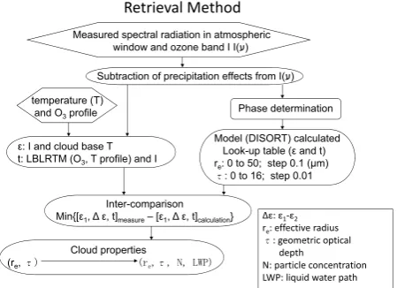
Fig. 1. Diagram illustrating the cloud property retrieval method. The

parametersre,τ,ε,t,Nand WP represent effective radius, visible

optical depth, cloud emissivity, cloud transmittance, particle con-centration and water path, respectively. Cloud phase is determined first based on cloud spectral emissivity and cloud base brightness temperature. A look-up table includingεandtfor a range ofreand

τ is computed with DISORT for the corresponding phase. Calcu-latedεandtare obtained based on measurements. A minimisation of the difference between calculatedεandtand values in the look-up table is used to obtainreandτ. CloudN and WP are obtained

based on a log-normal size distribution and the retrieved values of

reandτ.

The retrieval process has several important components. Narrow bands or ’micro-windows’ are selected in the atmo-spheric window and ozone band where atmoatmo-spheric water vapour emission is particularly small. It is by comparing measured values of cloud transmissivity and emissivity in these micro-windows to theoretically estimated values that cloud phase, effective radius and optical depth are inferred. These quantities can be combined to provide cloud water path and, in combination with estimates of cloud thickness, cloud particle concentration. The full retrieval algorithm, in-cluding our modifications is illustrated in Fig. 1.

2.1 Micro-window selection

For purposes of measurement and calculation of cloud win-dow emissivity, M01 identified seven micro-winwin-dows with a width of 2 cm−1_{where water vapour absorption is} particu-larly small and with varying sensitivity of particle absorption efficiencyQabs, to particle radius. As shown in Fig. 2,

(3)

5000 600 700 800 900 1000 1100 1200 20

40 60 80 100

cloudy

clear

ν (cm−1₎

I (mw m

−

2 sr cm

−

1)

8000 850 900 950 1000 5

10 15 20 25 30 35

830.7 862.5 903.5 935.8 960.4 988.4 917.5

cloudy

clear

ν (cm−1₎

I (mw m

−

2 sr cm

−

1)

Fig. 2. Selected micro-windows in the atmospheric window, at which atmospheric gases absorption is particularly small. The upper and lower

spectral radiation are for cloudy and clear conditions, respectively, measured at ARM NSA-AAO on 7 May 2001.

100 ₁₀1 ₁₀2

0 0.2 0.4 0.6 0.8 1 1.2 1.4

Qabs

re (µm)

a b

c d e fg

water

ν (cm−1) a=830.7 b=862.5 c=903.5 d=917.5 e=935.8 f=960.4 g=988.4

100 ₁₀1 ₁₀2

0 0.2 0.4 0.6 0.8 1 1.2 1.4

Qabs

a b

c d

e

f g

ice

ν (cm−1₎

a=830.7 b=862.5 c=903.5 d=917.5 e=935.8 f=960.4 g=988.4

re (µm)

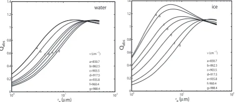
Fig. 3. Water and ice absorption efficiencyQ_abs as a function of cloud particle effective sizereat six different wavenumbers within

atmospheric micro-windows where atmospheric gaseous absorption is particularly small.

date micro-windows in the atmospheric window are centred at 830.7 (a), 862.5 (b), 903.5 (c), 917.5 (d), 935.8 (e), 960.4 (f) and 988.4 (g) cm−1. The values of liquid water and ice

Qabsare computed from Mie theory (Wiscombe, 1980) based on their respective complex refractive indices (Warren, 1984; Wieliczka et al., 1989). It is from this set that we determine pairs for which, as shown in Fig. 3, there is varying sensi-tivity of the water and ice absorption coefficient (Qabs) for a particularly wide range of particle radii (r) (r here, as it is applied to ice crystals, is more a radiative length scale than a spherical radius).

As shown in Fig. 3, the sensitivity ofQabstor is not the same in every micro-window. To exploit differences in size sensitivity, the retrieval method applied here uses the micro-window wavenumber pair 862.5 (b) and 935.8 cm−1(e). For these wavenumbers, a look-up table is calculated for cloud emissivityεin the two micro-windows, and cloud transmit-tance in the ozone bandt, for various values ofreandτ for a range of effective radiire<50 µm and visible optical depths

τ <16, using the Discrete Ordinates Radiative Transfer code

(DISORT; Stamnes et al., 1988). Emissivity and

transmissiv-ity are defined by

ε(ν)=I (ν)/B(Tc, ν) (1)

t=1−ε (2)

whereI is the radiative intensity andB(Tc)is the intensity of blackbody radiation for cloud base temperatureTc. The calculated value ofε (ν)is an “effective emissivity” that im-plicitly incorporates the small added component from reflec-tion, normally of order 2 % (see Turner, 2005). Calculated this way, the calculated effective emissivity is more directly comparable to ground-based measurements of downwelling

I (ν), which also implicitly incorporate both thermal

emis-sion and reflection.

Figures 4 and 5 shows micro-windowt(between 1038 and 1042 cm−1_{), alongside the aforementioned}_ε_{pairs and their} differenceεb−εe. Values are calculated with DISORT, as a

function ofreandτ, for both liquid and ice clouds.

The choice of the εb−εe split-window has several

strengths. First, the choice ofεbandεegives broad sensitivity

to a wide range of values ofreandτ for both liquid and ice clouds, although sensitivity diminishes for values ofrelarger than about 25 µm. For the purpose of retrievals, we can as-sume sensitivity for a range of parameter space bounded by a cloud transmissivity within the ozone bandtthat is greater than 0.05, and a cloud emissivityεbat 862.5 cm−1that is less than 0.95 and greater than 0.05.

The second strength is that the relationship of eitherreor

(4)

0 0.5 1 0

0.05 0.1 0.15 0.2

ICE

5 µm

10 µm

25 µm

50 µm

b

−

e

0 0.5 1

0 0.05 0.1 0.15 0.2

LIQUID

2 µm

5 µm

10 µm

20 µm

b

−

e

0 0.5 1

0 0.05 0.1 0.15 0.2

ICE

16

0.5

t_ozone

b

−

e

0 0.5 1

0 0.05 0.1 0.15 0.2

t_ozone

b

−

e

LIQUID

16

0.5

Fig. 4. “Arch plots” of split window cloud emissivity at 862.5 cm−1

(εb) and 935.8 cm−1 (εe), and cloud transmittance at 1040 cm−1 (tozone) for liquid and ice clouds, for a spread in effective radiire

(dashed: as labelled) and optical depthsτ(solid: 0.5, 1, 2, 4, 8, 16).

0 0.05 0.1 0.15 0.2 0

0.05 0.1 0.15 0.2

liquid _b − _e

ice

b

−

e

8

16 0.5

5 µm

0.01 0.1 1

−0.16 −0.14 −0.12 −0.1 −0.08 −0.06 −0.04 −0.02 0

ice t_ozone

(ice

−

liquid)/ice

5 µm

25 µm 50 µm

Fig. 5. Left: Range ofre(dashed: 5 and 10 µm) andτ(solid: 0.5,

1, 2, 4, 8, 16) associated with the split-window differenceεb−εe, depending on whether a cloud is assumed to be liquid or ice. The dotted line represents 1:1 perfect correspondence. For example, a re=5 µm liquid droplet in a cloud with an optical depthτof 1 has a

split-window difference that is lower than an equivalent cloud com-posed of ice crystals. Right: The difference in transmissivity within the ozone band associated with cloud phase assumption as a func-tion of ozone band transmissivitytozoneand cloudre.

normally such clouds can safely be assumed to be liquid. The reason for the weak dependence of transmissivity on cloud phase is that the imaginary component of the refractive in-dex at 1040 cm−1 is close to 0.045 for both ice and water (Warren and Brandt, 2008).

2.2 Phase determination

Remote determination of cloud phase using infrared tech-niques makes use of a difference in refractive index between ice and water (e.g., Strabala et al., 1994; Turner et al., 2003;

1 1.1 1.2 1.3 1.4 1.5 1.6 1.7 1

1.1 1.2 1.3 1.4 1.5 1.6 1.7

Liquid Ice

Uncertain

= 1

b

/e

e/g

Fig. 6. An intercomparison of ratios of calculated cloud

emissivi-ties at 862.5 cm−1(εb), 935.8 cm−1(εe) and 988.4 cm−1(εg) for assumed liquid and ice clouds. Magenta and blue dashed lines de-lineate these ratios for a range of plausible parameter space inreand

τfor ice and liquid, respectively. Black lines delineate the separa-tion between diagnosed liquid, uncertain, and ice phase retrievals. The unity ratio of the axesχ=1 is shown by the dashed black line, indicating that a rough metric for ice phased clouds is thatχ <1.

King et al., 2004; Chylek et al., 2006; Riedi et al., 2007; Nasiri and Kahn, 2008). Strictly, what is retrieved is a cloud phase that is “radiative” rather than microphysical. For ex-ample, it is common for liquid clouds in the Arctic to contain precipitating snow crystals (Hobbs and Rangno, 1998a; Pinto et al., 2001; McFarquhar et al., 2011). Snow crystals, while larger than droplets, are found in much lower concentra-tions and make a near negligible contribution to the total in-frared absorption cross-section density (e.g., will be shown in Fig. 7). From a radiative perspective, such clouds are purely liquid despite being microphysically “mixed-phased”.

One effective approach for phase identification has been to take advantage of pronounced spectral differences between liquid and ice in the far-infrared portion of the spectrum (Turner, 2005). The disadvantage is that retrievals tend to be constrained to drier atmospheres because strong rotational-band water vapour absorption contaminates the cloud sig-nal. Here we present in Fig. 6 a tri-spectral phase retrieval method that exploits differences in cloud emissivity within the atmospheric window, by focusing on narrow micro-windows where water vapour absorption is particularly small (Fig. 3). We have found that micro-windows at 862.5 cm−1 (εb), 935.8 cm−1 (εe) and 988.4cm−1 (εg) can be paired

to neatly separate cloud phase for much of the plausible space in (re, τ ). Figure 6 shows that a full range of

plau-sible parameter space in re and τ for ice and liquids lies neatly along two distinct lines in a space ofεb/εeandεe/εg.

(5)

Jan Mar May Jul Sep Nov 0

0.04 0.08 0.12

εP

Fig. 7. Seasonal variation in retrieved precipitation emissivity at

934.5 cm−1obtained at NSA-AAO between 2000 and 2003. Points are median values and bars the limits of the upper and lower quar-tiles.

χ=(εb/εe) / εe/εgare greater than unity, the cloud can be

identified as being liquid. The opposite is true for ice clouds. Clouds that are more spectrally flat, or in between ice and liquid, are not amenable to phase discrimination and are la-belled “uncertain”. In reality, many of these cases may in fact be “mixed-phased”. However, the ambiguity in the re-trieval prohibits us from identifying such clouds with cer-tainty. Nonetheless, as will be shown, retrievals of cloud properties are relatively insensitive to an a priori assessment of cloud phase, so retrievals of cloud properties are still per-formed where possible.

2.3 Estimation of cloud emissivity from measurements

In principle, cloud emissivity can be calculated from Eq. 1 using ground-based radiometer measurements of down-welling spectral radianceImeas(ν)combined with some esti-mate of cloud temperature. This works, provided that there is negligible emission by atmospheric constituents between the cloud and the ground.

We have chosen micro-windows where emission and ab-sorption of radiation by atmospheric gases is particularly small. However, cases can exist where below-cloud hydrom-eteors contribute non-negligibly to downwelling thermal ra-diance. To address this possibility, we first estimate a char-acteristic precipitation particle radius and number concentra-tion using a precipitaconcentra-tion retrieval method we previously de-veloped in Zhao and Garrett (2008). This technique retrieves precipitation microphysical properties as a function of radar reflectivity and Doppler velocity. The absorption (Qabs,P(ν)) and extinction (Qext,P(ν)) coefficients for precipitation can be computed from Mie theory (Wiscombe, 1980) based on the retrieved precipitation particle radius (r) and precipita-tion phase. From these values, precipitaprecipita-tion spectral emissiv-ity (εP(ν)) can be determined from

εP(ν)=1−exp(−

Z

1z

π Qext,P(ν)N r2dz) (3)

whereN is the precipitation particle concentration, and1z

is the depth of the precipitation layer.

For greatest precision, the below cloud contribution to downwelling radiance from water vapour could also be in-cluded. In this case, the corresponding emissivity εv(ν),

could in principle be calculated from Eq. 1 using a Line by Line Radiative Transfer Model (LBLRTM; Clough et al., 1992) based on measured ozone, temperature, and moisture profiles. Noting that transmittances multiply, the total emis-sivity of water vapour and precipitationεvP would be

εvP =εv+(1−εv) εP (4)

in which case, ignoring the second-order term inεvεP, the

corrected form of Eq. 1 for cloud emissivity is

ε (ν)=Imeas(ν)−εvP(ν) B (TP, ν)

(1−εvP) B (TC, ν)

(5) where Imeas(ν) is the surface measured radiation at wavenumberν, andB(TP, ν)andB(TC, ν)represent black-body radiation at ν for mean precipitation and cloud tem-peratureTP andTC; temperatures are estimated by match-ing detected heights to measured atmospheric temperature soundings. Here, for the sake of retrieval simplicity we make the approximation thatεvP 'εP. The associated error from

making this approximation is discussed in the appendix. With the contribution of precipitation to thermal emission excluded, the contribution of clouds and other trace gases to downwelling surface radiance is

IC(ν)=ε (ν) B (TC, ν) (6)

Figure 7 shows values ofεP obtained near Barrow, Alaska based on precipitation properties derived by Zhao and Gar-rett (2008). Retrieved values ofεP range from 0 to 0.14 with lower and upper quartile values of 0.01 and 0.04, respec-tively. Because values ofεP are generally low, the combined contribution of water vapour and precipitation toIcis

typi-cally about 1 %, in which case it can usually be ignored for the purpose of retrieving cloud properties. However, in the upper quartile, precipitation has a thermal emissivity greater than 0.05, and contributes in excess of 3 % to Isky. There-fore, if a higher certainty of accuracy is desired, thermally based cloud retrievals should systematically account for the precipitation radiation contribution.

2.4 Estimation of cloud transmissivity from

measurements

In order to constrain estimates of cloud emissivity, it helps to have an estimate of cloud transmissivitytsince, to first order,

ε=1−t. Cloud transmissivity is often estimated using the sun as a direct source. The drawback is that the sun can be absent for long stretches of time in the Arctic.

(6)

950 1000 1050 1100 0

30 60 210 240 270

(a

I (mW/(m

2 sr cm

−

1 ))

cb

(K)

950 1000 1050 1100

0 0.5 1

(c

ν (cm−1) t c

T

(b

950 1000 1050 1100

P

R

Q

Fig. 8. The steps used to determine cloud transmittance of ozone

downwelling emission in a 1038–1042 cm−1micro-window. (Top): The brightness temperatureTcbat cloud base is calculated on both

sides of the ozone emission band, at 970–990 cm−1 and 1070– 1100 cm−1). Then, the cloud brightness temperature Tcb within

the P and R branches of the ozone band is obtained using lin-ear interpolation. (Middle): The background radiance Ibkg from

non-ozone sources is calculated from the estimated cloud bright-ness temperatures. (Bottom): The transmissivity t in the P and R branches of the ozone band is calculated from the measured downwelling radianceIsky (corrected for precipitation

contribu-tions) fromt= Isky−Ibkg

/Iclear, whereIclear is the clear sky

downwelling radiance estimated from ozone, temperature and mois-ture profiles. Transmissivity values within the central Q branch between 1040 cm−1 and 1048 cm−1are estimated by interpolat-ing between the two regions delimited by dashed lines. Values of tozone are derived from a subset of transmissivity values within a

1038–1042 cm−1micro-window where water vapour absorption is small. The data shown is from measurements at ARM NSA-AAO on 15 July 2000.

emission within a 1038 cm−1to 1042 cm−1 micro-window. Because ground based measurements of downwelling radia-tion include both cloud and precipitaradia-tion emission and ozone transmission, cloud and precipitation emission must first be subtracted to obtain the ozone signal. Transmissivity can then be obtained if atmospheric ozone, temperature and moisture profiles are known. The ozone signal is isolated by examin-ing transmissivity within a narrow micro-window for water vapor emission is small.

The procedure for estimating cloud transmissivity within the 1038 cm−1to 1042 cm−1micro-window follows a series

of steps illustrated in Fig. 8. In the first step, surface radi-ance measurementsImeas(ν)are corrected for precipitation emission to give

Isky(ν)=Imeas(ν)−εP(ν) B (TP, ν) (7)

In the second step, a wavelength dependent brightness temperature Tcb representative of cloud base is estimated from the relation Isky(ν)=B (Tcb, ν). Intensity measure-ments are evaluated in two ranges, between 960 cm−1 and 975 cm−1 and between 1070 cm−1 and 1085 cm−1. These spectral bands lie within the atmospheric window, but just outside the P and R branches of ozone emission.

In the third step, the prior estimates of brightness temper-ature from outside the ozone band are used to evaluate val-ues ofTcbwithin the P and R branches associated with ozone emission. This is done using simple linear interpolation. This calculated value ofTcbwithin the ozone band is used to es-timate the background radianceIbkg(ν)that comes from all other sources than ozone and precipitation, including clouds, water vapour and other greenhouse gases.

Fourth, cloud transmissivity t is calculated within the P and R branches of ozone emission. The calculated back-ground emission Ibkg is subtracted from measurements of downwelling emissionIskywithin the P and R branches. The difference is divided by calculated values of the clear sky downwelling radiance Iclear in the P and R branches that would be associated with an atmosphere without precipita-tion or clouds

t (ν)=Icloudy(ν) /Iclear(ν)=(Isky(ν)−Ibkg(ν))/Iclear(ν) (8)

Values ofIclear are estimated using the LBLRTM radiative transfer model and measured profiles of atmospheric ozone, temperature and moisture.

Fifth, values oftthat are calculated in two narrower spec-tral bands – 1020 cm−1 to 1040 cm−1 in the P branch and 1048 cm−1to 1065 cm−1in the R branch – are then used to interpolate values oft in the Q branch between 1040 cm−1 and 1048 cm−1, thereby completing estimates oftwithin the ozone band. Interpolation is used because ozone emission is weak within the Q branch.

Finally, the desired values of tozone are obtained from a subset of these ozone transmissivity values, evaluated within a micro-window between 1038 cm−1 _{and 1042 cm}−1_{. This} micro-window is chosen because water vapour absorption is particularly small in this band.

2.5 Retrieval of cloud properties

Cloud effective radius (re) and visible optical depth (τ) can now be obtained in a two step process. First observed values ofεb,εe andεgare calculated from measured downwelling

(7)

Then, the observed values of εb andεe, along with ob-served values oftin the ozone band micro-window, are com-pared to those in a look-up table forre andτ for either ice or liquid clouds. Calculations are a simple least-squares min-imisation of

|[εb, 1ε, t]observations− [εb, 1ε, t]calculations| (9)

where,1ε=εb−εe.

The variables in the minimisation algorithm are weighted according to the relative magnitudes of their uncertainties. Uncertainties in ε result mostly from uncertainties in esti-mates of cloud-base temperature and uncertainties in mea-surements of downwelling spectral radiance, due for example to water vapour emission. In the latter case, these uncertain-ties are expected to manifest themselves as a bias. Values of

1ε, on the other hand, are highly robust to errors in temper-ature estimates, so they are weighted five times higher than emissivityεb. Cloud transmittance (t) is weighted three times

higher thanεbbecause it is comparatively insensitive to

certainties in estimated cloud phase. For clouds with an un-certain phase, retrievals of cloud properties are made assum-ing that the clouds are liquid. The assumption is that many “uncertain” clouds are in fact mixed-phased, in which case most of the cloud water path (and thermal emission) comes from high concentrations of small liquid droplets (Hobbs and Rangno, 1998b). In any case, as will be shown, retrievals tend not to be highly sensitive to this choice.

By assuming a log-normal cloud particle size distribution, such cloud properties as water path WP and particle number concentrationN, are related to retrievedreandτ through

W P=2ρreτ/3 (10)

N=3 exp(3σ2)WP/(4πρr_e31H ) (11) whereρis the water or ice density depending on the phase,

σ the assumed standard log-normal deviation of the particle size distribution, and 1H=Htop−Hbase is the difference between the measured cloud-top and -base heights.

We estimate a suitable value forσ of 0.32±0.10 based on a reanalysis of airborne measurements of particle size distri-butions<50 µm diameter obtained with an FSSP-100 during four University of Washington field campaigns in the Arc-tic between 1982 and 1998 (Garrett et al., 2004). It is more difficult to obtain a representative value for ice clouds, in part due to concerns about aircraft instrument performance (Field et al., 2003), but the value of σ is not necessarily markedly different (e.g., Rangno and Hobbs, 2001, Fig. 8). Accordingly,σ for ice and liquid are assumed to be identi-cal, but with an uncertainty for ice that is twice as large, i.e.,

σ=0.32±0.20.

Generally it is accepted that saturation effects limit in-frared retrieval techniques to values of WP lower than about

40 g m−2_{(Garrett et al., 2002), but this is not always the case.} The imaginary component of the refractive index is 0.046 for both ice and water in the portion of the ozone trans-mission band between 1038 cm−1and 1042 cm−1(Warren, 1984; Wieliczka et al., 1989). Therefore, in a bulk water medium, an ozone band transmittance value of 0.05, which is the lower sensitivity cutoff in the infrared retrieval tech-nique used here, should correspond to a liquid water absorp-tion path of 60 g m−2. Sensitivity to liquid water path can even extend beyond 60 g m−2if cloud particle radii are larger than about 10 µm (Fig. 4). The reason is that the skin depth for droplet absorption is smaller than the droplet radius itself. Any incident radiation is absorbed almost completely by the droplet exterior such that the interior is effectively invisible to the incident infrared radiation. The consequence is that the water path of a cloud can be higher before the cloud approx-imates a blackbody.

3 Measurements

The datasets used in this study are from the DOE Atmo-spheric Radiation Measurement (ARM) Programme North Slope of Alaska – Adjacent Arctic Ocean (NSA-AAO) site, the NOAA Global Monitoring Division (GMD), the European Remote Sensing satellite (ERS) Global Ozone Monitoring Experiment (GOME), the European Centre for Medium-Range Weather Forecasts (ECMWF), and the Na-tional Weather Service (NWS). The period of data acquisi-tion is 2000 to 2003 to be consistent with analysis described in Garrett and Zhao (2006). For analysis, measurements were grouped into five minute intervals. All ground-based data used here were obtained near Barrow, Alaska. Table 1 sum-marises the measurement site, instruments, resolution and ac-curacy.

1. Cloud Remote Sensing Measurements

Cloud properties were measured using a combination of active and passive remote sensors. Key instruments used for cloud retrievals from NSA-AAO include the Vaisala 25K Laser Ceilometer, the Micropulse Lidar, the Atmo-spheric Emitted Radiance Interferometer (AERI), and the millimetre wavelength cloud radar (MMCR) (Pep-pler et al., 2008).

(8)

clouds this corresponds to uncertainties better than 0.5 mW/(m2sr cm−1₎_.

A Vaisala Laser Ceilometer is used to determine cloud base, separate from precipitation, from sharp gradients in backscatter, and with an uncertainty of 7.6 m (Dong et al., 2005). Since its accuracy diminishes with height (Jay Mace personal communication), retrievals are re-stricted here to clouds with bases less than 4000 m altitude. The micropulse lidar (MPL) provides cloud boundaries with a height resolution of 30 m (Camp-bell et al., 2002). Where the MPL is attenuated, the Millimetre-wave Cloud Radar (MMCR) provides pro-files of radar reflectivity with measurement uncertain-ties of 0.5 dB. MMCR estimates of cloud boundaries have an accuracy of 45 m (Dong and Mace, 2003a). Here the MPL and MMCR are also used to exclude cases with multiple cloud layers (for example cirrus over stratus). More complicated scenes with multi-layered liquid clouds and ice crystal precipitation fill-ing the vertical space between layers are interpreted as single layer clouds.

We found that the ceilometer occasionally detects the base of a thin cloud that is invisible to the radar; or, if the cloud precipitates, the radar cloud top lies below the ceilometer cloud base. When this occurs, retrievals of cloud thickness and, hence, number concentrationNare impossible or nonsensical. However, estimates of other cloud properties are still performed since they do not rely on cloud thickness measurements.

For the purpose of a later comparison with the proposed thermal retrieval method, values of column-integrated liquid water path (LWP) are derived from brightness temperatures measured with a microwave radiometer (MWR) (Liljegren et al., 2001). The root-mean-square uncertainties of the LWP retrievals are commonly be-tween 10 g m−2 and 15 g m−2, but can be higher than 30 g m−2(Marchand et al., 2003).

2. Atmospheric Ozone, Temperature and Moisture Calculation of cloudy transmissiontof ozone emission requires profiles of atmospheric ozone, temperature and moisture. Surface ozone concentrations are provided from ultraviolet ozone photometers at the GMD site at Barrow, Alaska. Stratospheric ozone profiles (>6 km) are the assimilated ERS-GOME 3-D ozone distribu-tions from the World Data Center for Remote Sens-ing of the Atmosphere, WDC-RSAT (?). Ozone profiles from the surface to 6 km are obtained by interpolating between GOME stratospheric ozone profiles and GMD surface ozone measurements assuming a standard sea-sonal ozone profile. The time resolution for ozone pro-file measurements is 6 h and hourly at the surface. The accuracy of satellite measured profiles of stratospheric ozone concentration is about 5–10 % (∼100 ppb)

(La-paolo et al., 2007), and the accuracy of surface ozone concentration measurements from GMD is about 2 %. Temperature and moisture profiles are obtained from twice-daily NWS balloon-borne profiles up to the maxi-mum measured altitude – typically about 16 km. Above that level, European Center for Medium range Weather Forecasting (ECMWF) ERA-40 reanalyses are used (Uppala et al., 2005). Above 60 km, temperatures and humidities are fixed to 230 K and 5 ppmv. For times in-termediate to the NWS profile intervals, a temporal lear interpolation is applied to the data. For heights in-termediate to measured profile levels, cloud base and cloud top temperatures are obtained by applying a verti-cal linear interpolation. For the purpose of retrievals, we assume that balloon-sonde tropospheric water vapour measurements have an uncertainty of 15 % and that the measured upper-level temperature profiles have an un-certainty of 5 %, or roughly±12 K.

In the troposphere, temperature profiles are important for assessing cloud temperature. Based on observed temperature variability during the diurnal cycle, uncer-tainties in cloud base and cloud top temperatures are estimated to be±3 K. Other trace gases, such as carbon dioxide (CO2) and methane (CH4) do not have primary absorption bands at the frequencies used here. Associ-ated uncertainties in cloud property retrievals are less than 1 % and are not considered in detail.

4 Error analysis

Sources of uncertainty in retrievals come from both the mea-surements and the retrieval technique itself. To calculate the magnitude of the errors that are specific to the retrieval tech-nique, the technique is tested on synthetically created clouds. These errors are then combined with errors in the technique associated with measurement uncertainties. The intent here is to evaluate the extent to which adequate physics was im-plemented correctly in the algorithm development.

We test the ability of the retrieval technique to accu-rately infer synthetically specified values of cloud properties. Downwelling spectral radiance (I) at the surface is calculated using DISORT based on synthetically specified values ofre,

τ,Hbase,Htopand cloud temperature. From the values ofI, the cloud propertiesreandτ are “retrieved” and compared with the synthetic values.

(9)

Figure 10 shows that “retrieved” cloud properties agree very well with the synthetic values. Errors associated with retrievals ofτ are not shown since they are<2 % throughout the parameter space inre andτ. Forre, LWP, andN, com-puted values of 95 % confidence retrieval errors associated with the method exceed 10 % only where values ofreexceed 30 µm and values ofτ exceed about 6, presumably because

Qabsis only a weak function ofreand the sensitivity of cloud emissivity toτ decreases as a cloud thickens to approximate a blackbody. That we have assumed that clouds are micro-physically homogeneous in the vertical may mean that addi-tional errors are associated with true clouds. Retrievals based on cloud transmissivity of downwelling atmospheric radia-tion will tend to be biased by the microphysics at cloud top since this is near where radiative attenuation is a maximum; retrievals based on cloud thermal emission will be biased by properties at cloud base. Because the retrievals here are based on both emission and transmission, derived properties are ex-pected to represent some radiative average of the vertical pro-file.

The primary uncertainties in the retrievals arise from mea-surement errors. Based on the discussion of meamea-surement ac-curacies in Sect. 3, the 95 % confidence uncertainties in cloud base temperature (Tc), AERI radiance (I), water vapour pro-file (H2O), ozone profile (O3) and cloud depth (1H) are estimated to be about±3 K, 0.5 mW/(m2sr cm−1), 15 %, 100 ppb, and 50 m, respectively. Uncertainties in strato-spheric temperature and moisture profiles are 5 %. Aircraft measurements from the FIRE-ACE field campaigns show un-certainty in the cloud particle log-normal distribution spec-tral width (σ) to be±0.10 for liquid clouds (Garrett et al., 2004), and it is assumed to be±0.20 for ice clouds.

Assuming that errors from measurements of Tc, I, O3,

1H and σ are independent, the 1-sigma retrieval error in property x due to combined measurement and retrieval method errors is

σ_x2=σ_M2(∂x

∂M)

2₊_σ2

I(

∂x

∂I)

2₊_σ2

H2O(

∂x

∂H2O)

2₊_σ2 O3(

∂x

∂O3)

2

+σ_T2(∂x

∂T)

2₊_σ2

1h(

∂x

∂1H)

2₊_σ2

σ(

∂x

∂σ)

2 ₍₁₂₎

whereσy is the standard deviation of variabley,M

repre-sents the retrieval method, andI, H2O, O3,T,1Handσare measurement variables, the brackets()contain the sensitiv-ity ofx to the measurements or retrieval method. Here, the covariance between the different quantities is assumed to be zero because the measurements are independent.

Table 2 shows estimates of the liquid and ice cloud re-trieval errors due to combined uncertainties in the rere-trieval method and measurements. The errors inre,τ, and WP are due mainly to uncertainties in cloud base temperature and AERI radiance. Errors inN are also strongly dependent on uncertainties in cloud depth and the standard deviation of the droplet or ice size distribution. The combined 95 % confi-dence uncertainties in cloudre,τ, and WP are about 10 %,

0 2000 4000 6000 8000

0 10 20 30 40 50 60

O₃ (ppb)

H (km)

Jan 15, 2001

210 220 230 240 250 260 270

0 10 20 30 40 50 60

T (K)

H (km)

Jan15, 2001

0 2000 4000 6000 8000

0 10 20 30 40 50 60

O₃ (ppb)

H (km)

May 7, 2000

210 220 230 240 250 260 270

0 10 20 30 40 50 60

T (K)

H (km)

May 7, 2000

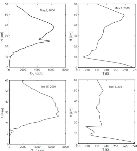
Fig. 9. Ozone (left) and temperature (right) profiles at Barrow,

Alaska, obtained on 7 May 2000 (above) and 15 January 2001 (be-low).

20 %, and 16 %. ForN, they are 38 % and 55 % for liquid and ice, respectively.

5 Evaluation

5.1 Comparison with measurements

Using the phase identification method employed here, it was possible to identify whether the cloud phase was liquid or ice in 65 % of cases where there were thin clouds with

0.05< εb<0.95. The remainder of cases were classified as

having an uncertain phase. One way to assess the magnitude of error in the cloud phase determination is to examine the detected phase above and below certain known phase transi-tions, such as the melting and homogeneous freezing points. For thin cloud cases with cloud top temperatures higher than 273 K, clouds were classified as being ice in 6 % of cases and liquid in 45 % of cases, the remainder being uncertain. The respective numbers for clouds with base temperatures below 238 K were 73 % and 11 %. These numbers suggest that, in about 10 % of cases where a phase identification was made, the phase was misclassified.

(10)

Table 1. Site, instrument, resolution, and 95 % confidence accuracy of measurements used in this study.

Source Instrument Data resolution Accuracy

ERS- Satellite

GOME Spectrometer Stratospheric O3profile 6 h 5–10 %

GMD Photometers Surface ozone 1 h 2 %

NWS Rawinsonde Temperature Profile 12 h 3 K

NWS Rawinsonde Water vapor Profile 12 h 15 %

ECMWF Simulation Temperature Profile 6 h 3 K

ECMWF Simulation Water vapor Profile 6 h 15 %

ARM AERI Surface Radiation 450 s 0.5 mW/(m2sr cm−1)

ARM Laser/Ceilometer Cloud Base 36 s 7.6 m

ARM MMCR Radar Radar Reflectivity 36 s 0.5 dB

ARM MMCR Radar Cloud Top 36 s 45 m

ARM MMCR Radar Doppler velocity 36 s 0.1 m s−1

ARM MWR Liquid water path 15 s 30 g m−2

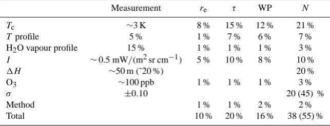
Table 2. Typical 95 % confidence retrieval errors for liquid and (ice) cloudre,τ, WP andNbased on combined measurement and retrieval

errors.

Measurement re τ WP N

Tc ∼3 K 8 % 15 % 12 % 21 %

T profile 5 % 1 % 7 % 6 % 7 %

H₂O vapour profile 15 % 1 % 1 % 1 % 3 %

I ∼0.5 mW/(m2sr cm−1) 5 % 10 % 8 % 10 %

1H ∼50 m (˜20 %) 20 %

O3 ∼100 ppb 1 % 1 % 1 % 3 %

σ ±0.10 20 (45) %

Method 1 % 1 % 2 % 2 %

Total 10 % 20 % 16 % 38 (55) %

values of LWP and IWP using the infrared-based method and the LWP derived from the MWR, evaluated for all cases where comparisons were possible. What is shown is a fairly high correlation (r2=0.50) between microwave and thermal IR retrievals of LWP, but with a 10 g m−2 to 15 g m−2 pos-itive bias in the MWR LWP measurements, consistent with known uncertainties in the MWR retrievals (Marchand et al., 2003). By comparison, thermal retrievals of IWP and the MWR LWP do not correlate well (r2=0.06). When the in-frared based retrievals of IWP are non-zero, the MWR LWP retrievals are consistently within MWR uncertainty bounds.

For those cases where the retrieved cloud phase is “uncer-tain”, it may nonetheless be possible to retrieve cloud optical depthτ and effective radiusreto within an acceptable degree of confidence. Figure 12 shows a comparison between the values of retrievedτ andrefor “uncertain” cases depending on whether the cloud optical properties are treated as being either liquid or ice. For example, if the cloud were composed of ice, but the cloud microphysics were calculated as if it were liquid, then the optical depth would be overestimated, and the effective radius would be underestimated, by about 15 %. These additional uncertainties are comparable to those

due to measurement errors where the cloud phase has been correctly determined (Table 2).

5.2 Comparison with independent retrievals

The final comparison is between the infrared-based retrieval approach described here and an independent retrieval ap-proach that has been applied to the same time period and location by Dong and Mace (2003b). The Dong and Mace method is based on ground pyrometer measurements of solar shortwave cloud transmissivity and MWR retrievals of liquid water path. Combined with the solar zenith angle and mea-surements of surface albedo, Dong and Mace applied their technique to retrieve liquid cloud optical depth, cloud droplet effective radius, and cloud droplet number concentration.

(11)

Visible Optical Depth

2 4 6 8 10 12 14 16 5

10 15 20 25 30 35 40 45 50

1 5 10

r ( m)e

μ

r ( m)

2 4 6 8 10 12 14 16 5

10 15 20 25 30 35 40 45 50

1 5

5 10 10

e

μ

b) LWP

2 4 6 8 10 12 14 16 5

10 15 20 25 30 35 40 45 50

1 5

10 20 30

r ( m)e

μ

c) N

a) re

Fig. 10. Calculated uncertainties in retrievals of liquid cloudre, LWP andNthat are associated only with the look-up table method outlined

in Sect. 4, separate from any errors associated with uncertainties in measurements. Errors (contours) are expressed in percent within a space ofreanτfor a cloud with fixed boundaries and a specified atmospheric profile.

−010 0 10 20 30 40 50 60

10 20 30 40 50 60

MWR LWP (g m−2)

Retrieved LWP and IWP (g m

−

2)

Ice

r2 =0.06

Liquid

r2 =0.5

Fig. 11. Linear probability density distributions (contours) for an

inter-comparison of retrieved and Microwave Radiometer (MWR) measured LWP. The dashed line is a 1:1 line.

For the sake of intercomparison, we examined how well microphysics retrievals agreed for an intermediate regime between 20 g m−2 and 40 g m−2, as shown in Fig. 13. For a period between May and September, the average LWP within this range was 29.26 g m−2 for the infrared method and 29.62 g m−2for the Dong and Mace method.

Overall, both techniques give very similar retrievals, at least in trends if not always in absolute values. Both ap-proaches reveal a transition in liquid cloudre between late spring and summer from approximately 5 µm to 10 µm along with a commensurate relative decline in optical depth. How-ever, in late spring, the Dong and Mace retrievals ofretend to be about one to two micrometers smaller, and this lends it-self to as much as a factor of three discrepancy in retrievals of droplet number concentration (Eq. 11). Nonetheless the tran-sition to higher droplet concentrations between spring and summer is reproduced by both methods. In summer, the dif-ferences between both approaches are in general very small.

Optical depth

Effective radius (µm)

Liquid

Ice

0 5 10 15 20 25

Fig. 12. Linear probability density distributions (contours) for

trieved clouds of “uncertain” phase depending on whether the re-fractive indices in the retrievals are assumed to be those of ice or liquid. The dashed line is a 1:1 line.

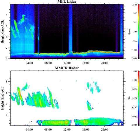
5.3 Case study

Figure 14 shows lidar and radar imagery from NSA-AAO for a scene on 13 January 2001 that is both complex while not being unusual. The day is characterised by two cloud layers: a high layer above 4 km altitude that resembles cirrus fall-streaks, and a lower thin cloud layer at around 1 km altitude with precipitation falling beneath.

Fig. 15 shows retrieved cloud properties for this case. What is observed is a high cirrus cloud in the beginnings of the day that, with some overlap, transitions to a thin low-level cloud. Because the cirrus and lower-low-level cloud are well separated, cloud retrievals are made here even though the day is largely multi-layered. With a few exceptions, when cloud phase is explicitly retrieved, it indicates that the cirrus cloud is ice and the low-level cloud is liquid. The spectral slope

χ=(εb/εe) / εe/εg

(12)

May Jun Jul Aug Sep 0

5 10 15 20

re

(

µ

m)

This Study Dong and Mace

May Jun Jul Aug Sep

0 5 10 15

τ

May Jun Jul Aug Sep

100 101 102 103

Month

N (cm

−

3)

Fig. 13. Calculated in 10-day intervals for the period May to

September between 2000 and 2003, retrieved cloud droplet effec-tive radiusre, visible optical depthτ, particle number concentration

N, using two methods: the method described here (black), and an independent technique based on shortwave transmission and MWR LWP retrievals developed by Dong and Mace (2003b). For the in-tercomparison, retrievals are constrained to a range of LWP values between 20 g m−2and 40 g m−2. Bars represent the range in quar-tiles.

is relatively consistent within each of these two regions: the low-level cloud has median and (lower, upper] quartile val-ues ofχthat are 1.04 (1.03 1.05) versus 0.90 (0.85 0.93) in the cirrus.

Median and (lower, upper) quartile values for the low-level liquid cloud properties are a thickness of 250 (236 272) m, an emissivity of 0.90 (0.83 0.93), a visible optical depth of 6.1 (5.1 7.2], a droplet effective radius of 4.7 (3.8 6.2) µm, droplet concentrations of 192 (130 434) cm−3_{, and a liquid} water path of 22 (15 25) g m−2. For the ice crystal cirrus, me-dian and (lower, upper) quartile values are a thickness of 589 (237 930) m, an emissivity of 0.09 (0.07 0.16), a visible op-tical depth of 0.20 (0.16 0.35), an ice crystal effective radius of 48 (39 49) µm, ice crystal concentrations of 69 (47 128) litre−1, and a liquid water path of 6.1 (4.9 8.0) g m−2. Given that the ice crystal effective radius retrieval is near the upper limit for retrieval sensitivity of 50 µm, it is possible that the true sizes are larger and the concentrations lower.

04:00 08:00 12:00 16:00 20:00

0 2 4 6 8

Height (km) AGL

MPL Lidar

-20.00 -14.17 -8.33 -2.50 3.33 9.17 15.00

Signal

04:00 08:00 12:00 16:00 20:00

2 4 6 8

Height (km) AGL

MMCR Radar

-60.00 -50.83 -41.67 -32.50 -23.33 -14.17 -5.00

dBz

Fig. 14. Lidar and radar returns from NSA-AAO on 13 January,

2001.

5.4 Seasonal variability

Figure 16 shows the retrieved seasonable variability in thin cloud properties at NSA-AAO between 2000 and 2003, pre-sented as monthly means. Cloud cover statistics are prepre-sented for both all clouds and those graybody clouds withεb<0.95. The remainder of parameters shown apply only to graybody clouds for which the thermal IR retrieval technique presented here applies. Therefore, the statistics do not represent a true climatology since they omit thicker clouds that radiate as blackbodies.

In general, the statistics are qualitatively consistent with prior studies of the seasonality of Arctic clouds (e.g., Shupe et al., 2005; Kay and Gettelman, 2009; Devasthale et al., 2011). The Arctic is cloudy. Thin graybody clouds are a sub-stantial fraction of the total, comprising about 42 %. On av-erage, these clouds are found at low levels with bases below 2 km altitude. In summer when conditions are warmer, the first cloud layer viewed from the ground is rarely ice. Also in summer, clouds have a higher water path and are more op-tically thick than in winter. Included for comparison is the seasonal cycle in the MWR liquid water path, which shows that the magnitude of the LWP cycle for both thick and thin clouds approaches a factor of ten. The optical depths and ef-fective radii of all gray-body clouds are intermediate to those of the liquid and ice clouds, but on average they are most closely approximated by the liquid cloud portion.

(13)

0.1 1 10

Height (km)

Base Top

1 10 100

re

(

µ

m)

0.1 1 10

0.1 10 1000

N (cm

−

3)

0 4 8 12 16 20 24 1

10 100

WP (gm

−

2)

Jan 13, 2001

0 0.5 1

,

t

0.6 0.8 1 1.2 1.4

Liquid Ice Uncertain

Fig. 15. Retrieved cloud boundariesH, emissivity (at 862.5 cm−1 ) and transmissivity (at 1040 cm−1), ratio of spectral slopesχ=

(εb/εe) / εe/εg, and cloud droplet effective radiusre, visible

op-tical depthτ, particle number concentrationN, and condensate wa-ter path WP, for the scene in Fig. 14 observed at NSA-AAO on 13 January 2001.

intercomparison, in-situ aircraft observations of ice crystal concentrations from the Arctic tend to be lower than those that are retrieved (e.g., Jouan et al., 2012). One reason for the discrepancy could be that analyses of in-situ ice crystal concentration measurements sometimes use an experimental algorithm that removes particles with unusually short inter-arrival times at airborne probes, assuming these particles arise from ice crystal shattering on instrument inlets. Pro-vided that these algorithms are appropriately applied, another possibility for the discrepancy is that the retrieval method discussed here is in error because it is limited to clouds (not below-cloud precipitation) with effective radii smaller than 50 µm: where ice crystal effective radii are in fact larger than 50 µm, retrieved ice crystal number concentrations could be erroneously high.

0 0.5 1

Cover

0 2 4

Boundaries (km)

0 0.2 0.4 0.6

Phase fraction

0 10 20 30 40 50

re

(

µ

m) All Liquid Ice

0 2 4 6

1 10 100

N (cm

−

3)

2 4 6 8 10 12

10 100

WP (g m

−

2)

Month

Fig. 16. Monthly averages of retrieved graybody cloud properties

for the 2000 to 2003 time period at NSA-AAO. Top panel: retrieved cloud cover of all (black) and graybody (gray) clouds. Lower pan-els: for graybody clouds only, the cloud boundaries, the fraction of clouds that were identified as liquid (blue) or ice (magenta), the cloud particle effective radiusreof liquid, ice and all (black) clouds,

the cloud optical depthτ, the cloud particle number concentration (liquid (cm−3), ice (cm−3)), and the water path WP. The dashed line for WP represents MWR retrievals for all liquid clouds.

6 Conclusions

A method has been developed for the retrieval of Arctic cloud microphysical and macrophysical properties based on cloudy thermal emission and stratospheric ozone cloudy thermal transmission. For both liquid and ice clouds, two emissiv-ity micro-windows are selected in the atmospheric window based on the sensitivity of the particle absorption coefficient to particle effective radiusre. Cloud micro-structure proper-ties are obtained by matching estimates of cloud emissivity and transmissivity from measurements with calculated val-ues from a look-up table. The retrieval technique is limited to graybody clouds with cloud optical depthsτ less than 16 and cloud particle effective radiiresmaller than 50 µm.

(14)

plausible space in(re, τ ). The phase retrieval reflects the ra-diative properties of the clouds: mixed-phased clouds might be identified as being liquid if the ice crystals contribute neg-ligibly to their thermal emission.

Error analysis indicates that the method’s main sources of retrieval error come from uncertainties in measured cloud base temperature, surface thermal radiance, and the strato-spheric ozone profile. Because retrievals are constrained by both cloud transmittance and emissivity, they display very low sensitivity to water vapour. The respective 95 % confi-dence retrieval errors inre, τ, WP, andN are about 10 %, 20 %, 16 % and 38 % for liquid cloud, and about 10 %, 20 %, 16 % and 55 % for ice clouds. The retrievals of cloud micro-physical properties require an a priori determination of cloud phase. Where phase cannot be determined, or is in error, the bias in retrievals ofreandτ is approximately 15 %.

The thermal IR based method described here is particu-larly well suited to optically thin clouds that can be difficult to characterise using other remote sensing approaches. For example, the average liquid water path retrieved by the mi-crowave radiometer (MWR) between the months of Novem-ber and February is 28 g m−2. Such clouds are optically thin in the thermal IR, but they lie within the MWR retrieval noise.

Also, retrieval methods based on solar transmission can be well suited for describing cloud properties in the summer (e.g., Dong and Mace, 2003a), but they are inapplicable dur-ing the winter night. By contrast, thermal emission is year round. The primary limitations of the thermal IR approach discussed here are twofold. First, it requires a fairly exten-sive grouping of measurements to achieve its stated level of accuracy. Second, it requires that clouds cannot approximate blackbodies. Clouds tend to be most optically thick in sum-mer when this method could be used in combination with other approaches.

Appendix A

Sensitivity to water vapour

For the emissivity measurement calculations described here, the contribution of water vapour to the measured signal is not subtracted (Eq. 6) because its contribution is, for the most part, negligible. Estimated retrieval uncertainties associated with water vapour were estimated to be within 1 % forτ,re and WP.

For comparison, a prior study by Turner (2005) described the “MIXCRA” algorithm, which, while highly flexible and accurate in its application of AERI measurements to Arctic cloud retrievals (Turner and Eloranta, 2008), was nonetheless constrained to scenes with precipitable water vapour (PWV) amounts less than 1 cm. This precondition could be removed, but only if the cloud phase was known a priori, as it was

0 5 10 15 20 25

10−1 100 101 102

std = 0.20 µm

r_e(WV) (µm)

Difference (%)

∆r_e<0.01µm: 86% 0 - 0.50.5 - 1 1 - 2 > 2 PWV (cm)

Fig. A1. Percent difference in retrievals ofre associated with not subtracting water vapor contributions to measured downwelling ra-diance in emissivity calculations (Eq. 6), versus retrieved values with water vapor subtracted, as a function of the precipitable water vapor content (PWV) of the atmosphere. The only differences plot-ted are those in the 14 % of cases with differences inre>0.01 µm. Negative differences are in closed circles.

only the phase identification component of MIXCRA that in-volved frequencies outside the atmospheric window.

By contrast, the retrievals described here, including those of phase, are based only on measurements within the atmo-spheric window where water lacks single-molecule rotational or vibrational fundamental modes. The disadvantage of this approach is that differences in the absorption properties of ice and liquid clouds are not always clearly separated. Also, wa-ter vapour continuum absorption does remain in the window. Nonetheless, water vapour emission is implicitly factored into the retrievals through comparisons of transmissivity in-side and just outin-side the 1040 cm−1ozone band that are used to calculate cloud transmissivity (Fig. 8). Moreover, cloud emissivity estimates are evaluated within “micro-windows” where atmospheric absorption and emission by water vapour is particularly small.

Figure A1, shows the influence of water vapour on the re-trievals ofre. Not subtracting water vapour in estimates of cloud emissivity causes differences in retrieved values ofre. In 86 % of cases the difference is less than 0.01 µm, which is the precision of the retrieval technique. In the remainder of cases the difference is generally still very small, in the vicin-ity of 1 to 2 percent. In only a very few cases is the difference in excess of 10 %, although still less than 1 µm.

(15)

with lower water vapour emission, but they are also associ-ated with thinner, less strongly emitting clouds. In this case, the contribution of water vapour to the measured signal may be much larger than is typical, if still small.

Acknowledgements. This work was supported by the National Science Foundation through grants 0303962 and 0649570, the Clean Air Task Force, through NOAA by grant 2308014, and the Ministry of Science and Technology of China through grant 2013CB955804. We are grateful to the late P. V. Hobbs for having provided aircraft data, the Word Data Center for Remote Sensing of the Atmosphere for ozone profile data, X. Dong for his cloud retrieval product, and Jay Mace and Sally Benson for plots of the lidar and radar signals.

Edited by: A. Kokhanovsky

References

Beesley, J. A.: Estimating the effect of clouds on the arctic surface energy budget, J. Geophys. Res., 105, 10103–10117, 2000. Bourdages, L., Duck, T. J., Lesins, G., Drummond, J. R., and

Elo-ranta, E. W.: Physical properties of High Arctic tropospheric particles during winter, Atmos. Chem. Phys., 9, 6881–6897, doi:10.5194/acp-9-6881-2009, 2009.

Campbell, J. R., Hlavka, D. L., Welton, E. J., Flynn, C. J., Turner, D. D., Spinhirne, J. D., and Scott, V. S.: Full-time eye-safe cloud and aerosol lidar observation at atmospheric radiation measure-ment program sites: Instrumeasure-ments and data processing, J. Atmos. Ocean. Tech., 19, 431–442, 2002.

Cesana, G., Kay, J. E., Chepfer, H., English, J. M., and de Boer, G.: Ubiquitous low-level liquid-containing Arctic clouds: New observations and climate model constraints from CALIPSO-GOCCP, Geophys. Res. Lett., 39, L20804, http://dx.doi.org/10. 1029/2012GL053385, 2012.

Chylek, P., Robinson, S., Dubey, M. K., King, M. D., Fu, Q., and Clodius, W. B.: Comparison of near-infrared and thermal in-frared cloud phase detections, J. Geophys. Res., 111, D20203, doi:10.1029/2006JD007140, 2006.

Clough, S. A., Iacono, M. J., and Moncet, J. L.: Line-by-line cal-culations of atmospheric fluxes and cooling rates: application to water vapour, J. Geophys. Res., 97, 15761–15785, 1992. Comstock, J. M., D’Entremont, R., DeSlover, D., Mace, G. G.,

Ma-trosov, S. Y., McFarlane, S. A., Minnis, P., Mitchell, D., Sassen, K., Shupe, M. D., et al.: An intercomparison of microphysical retrieval algorithms for upper-tropospheric ice clouds, Bull. Am. Meteorol. Soc., 88, 191–204, 2007.

Curry, J. A., Rossow, W. B., Randall, D., and Schramm, J. L.: Overview of Arctic cloud and radiation characteristics, J. Cli-mate, 9, 1731–1764, 1996.

Curry, J. A., Hobbs, P. V., King, M. D., Randall, D. A., Minnis, P., Isaac, G. A., Pinto, J. O., Uttal, T., Bucholtz, A., Cripe, D. G., Gerber, H., Fairall, C. W., Garrett, T. J., Hudson, J., Intrieri, J. M., Jakob, C., Jensen, T., Lawson, P., Marcotte, D., Nguyen, L., Pilewskie, P., Rangno, A., Rogers, D. C., Strawbridge, K. B., Valero, F. P. J., Williams, A. G., and Wylie, D.: FIRE Arctic Clouds Experiment, Bull. Amer. Meteor. Soc., 81, 5–29, 2000.

de Boer, G., Collins, W. D., Menon, S., and Long, C. N.: Using sur-face remote sensors to derive radiative characteristics of Mixed-Phase Clouds: an example from M-PACE, Atmos. Chem. Phys., 11, 11937–11949, doi:10.5194/acp-11-11937-2011, 2011. Dergach, A. L., Zabrodsky, G. M., and Morachevsky, V. G.: The

results of a complex investigation of the type St-Sc clouds and fogs in the Arctic, Bull. Acad. Sci. USSR, Geophys. Ser., 1, 66– 70, 1960.

Devasthale, A., Tjernstr¨om, M., Karlsson, K.-G., Thomas, M. A., Jones, C., Sedlar, J., and Omar, A. H.: The vertical distribu-tion of thin features over the Arctic analysed from CALIPSO observations Part I: Optically thin clouds, Tellus B, 63, 77–85, doi:10.1111/j.1600-0889.2010.00516.x, 2011.

Dong, X. and Mace, G. G.: Arctic stratus cloud properties and radia-tive forcing derived from ground-based data collected at Barrow, Alaska, J. Climate, 16, 445–461, 2003a.

Dong, X. and Mace, G. G.: Arctic stratus cloud properties and radia-tive forcing derived from ground-based data collected at Barrow, Alaska, J. Climate, 16, 445–461, 2003b.

Dong, X., Minnis, P., and Xi, B.: A climatology of midlatitude con-tinental clouds from the ARM SGP central facility: Part I: Low-level cloud macrophysical, microphysical, and radiative proper-ties, J. Climate, 18, 1391–1410, 2005.

Field, P. R., Wood, R., Brown, R. A., Kaye, P. H., Hirst, E., Green-way, R., and Smith, J. A.: Ice particle interarrival times measured with a Fast FSSP, J. Atmos. Ocean. Technol., 20, 249–261, 2003. Foot, J. S.: Some observations of the optical properties of clouds,

Part 2, Cirrus, Q. J. R. Meteorol. Soc., 114, 145–164, 1988. Francis, J. A. and Hunter, E.: New insight into the

dis-appearing Arctic sea ice, Eos Trans. AGU, 87, 509–511, doi:10.1029/2006EO460001, 2006.

Francis, J. A. and Hunter, E.: Changes in the fabric of the Arctic’s greenhouse blanket, Env. Res. Lett., 2, 045011–+, doi:10.1088/1748-9326/2/4/045011, 2007.

Fridlind, A. M., Ackerman, A. S., McFarquhar, G., Zhang, G., Poel-lot, M. R., DeMott, P. J., Prenni, A. J., and Heymsfield, A. J.: Ice properties of single-layer stratocumulus during the Mixed-Phase Arctic Cloud Experiment: 2. Model results, J. Geophys. Res., 112, D24202, doi:10.1029/2007JD008646, 2007.

Garrett, T. J. and Zhao, C.: Increased Arctic cloud longwave emis-sivity associated with pollution from mid-latitudes, Nature, 440, 787–789, doi:10.1038/nature04636, 2006.

Garrett, T. J., Radke, L. F., and Hobbs, P. V.: Aerosol effects on the cloud emissivity and surface longwave heating in the Arctic, J. Atmos. Sci., 59, 769–778, 2002.

Garrett, T. J., Zhao, C., Dong, X., Mace, G. G., and Hobbs, P. V.: Effects of varying aerosol regimes on low-level Arctic stratus, Geophys. Res. Lett., 31, 17105–17109, 2004.

Han, W., Stamnes, K., and Lubin, D.: Retrieval of surface and cloud properties in the Arctic from NOAA AVHRR measurements, J. Appl. Meteor., 38, 989–1012, 1999.

Hansen, J. E. and Travis, L. D.: Light scattering in planetary atmo-spheres, Space Sci. Rev., 16, 527–610, 1974.

Harrington, J. Y., Feingold, G., and Cotton, W. R.: Radiative im-pacts on the growth of a population of drops within simulated summertime Arctic stratus, J. Atmos. Sci., 57, 766–785, 2000. Hildenbrand, B., Bittner, M., Baier, F., and Erbertseder, T.:

(16)

pro-files by assimilating total column ozone data into the 3D-NCAR-ROSE chemical-transport model, 487–491, 2003.

Hobbs, P. V. and Rangno, A. L.: Microstructure of low and middle-level clouds over the beaufort sea, Q. J. R. Meteorol. Soc., 124, 2035–2071, 1998a.

Hobbs, P. V. and Rangno, A. L.: Microstructures of low and middle-level clouds over the Beaufort Sea, Quart. J. Roy. Meteor. Soc., 124, 2035–2071, 1998b.

Hobbs, P. V., Rangno, A. L., Shupe, M., and Uttal, T.: Airborne studies of cloud structures over the Arctic ocean comparisons with retrievals from ship-based remote sensing measurements, J. Geophys. Res., 106, 15029–15044, 2001.

Jayaweera, K. O. L. F. and Ohtake, T.: Concentration of ice crystals in Arctic Stratus Clouds, Geophys. Res. Lett., 9, 94–97, 1982. Jouan, C., Girard, E., Pelon, J., Gultepe, I., Delano¨e, J., and

Blanchet, J.-P.: Characterization of Arctic ice cloud proper-ties observed during ISDAC, J Geophys Res, 117, D23207, doi:10.1029/2012JD017889, 2012.

Jourdan, O., Mioche, G., Garrett, T. J., Schwarzenb¨ock, A., Vidot, J., Xie, Y., Shcherbakov, V., Yang, P., and Gayet, J.-F.: Coupling of the microphysical and optical properties of an Arctic nimbo-stratus cloud during the ASTAR 2004 experiment: Implications for light-scattering modeling, J. Geophys. Res., 115, D23206, doi:10.1029/2010JD014016, 2010.

Kay, J. E. and Gettelman, A.: Cloud influence on and response to seasonal Arctic sea ice loss, J. Geophys. Res., 114, D18204, doi:10.1029/2009JD011773, 2009.

Kay, J. E., L’Ecuyer, T., Gettelman, A., Stephens, G., and O’Dell, C.: The contribution of cloud and radiation anomalies to the 2007 Arctic sea ice extent minimum, Geophys. Res. Lett., 35, L08503, doi:10.1029/2008GL033451, 2008.

Kay, J. E., Holland, M. M., Bitz, C. M., Blanchard-Wrigglesworth, E., Gettelman, A., Conley, A., and Bailey, D.: The Influence of Local Feedbacks and Northward Heat Transport on the Equi-librium Arctic Climate Response to Increased Greenhouse Gas Forcing, J. Climate, 25, 5433–5450, doi:10.1175/JCLI-D-11-00622.1, http://dx.doi.org/10.1175/JCLI-D-11-doi:10.1175/JCLI-D-11-00622.1, 2012. King, M. D., Platnick, S., Yang, P., Arnold, G. T., Gray, M. A.,

Riedi, J. C., Ackerman, S. A., and Liou, K. N.: Remote sensing of liquid water and ice cloud optical thickness and effective radius in the Arctic: Application of airborne multispectral MAS data, J. Atmos. Ocean. Tech., 21, 857–875, 2004.

Klein, S. A., McCoy, R. B., Morrison, H., Ackerman, A. S., Avramov, A., Boer, G. d., Chen, M., Cole, J. N. S., Del Genio, A. D., Falk, M., Foster, M. J., Fridlind, A., Golaz, J.-C., Hashino, T., Harrington, J. Y., Hoose, C., Khairoutdinov, M. F., Larson, V. E., Liu, X., Luo, Y., McFarquhar, G. M., Menon, S., Neg-gers, R. A. J., Park, S., Poellot, M. R., Schmidt, J. M., Sednev, I., Shipway, B. J., Shupe, M. D., Spangenberg, D. A., Sud, Y. C., Turner, D. D., Veron, D. E., Salzen, K. v., Walker, G. K., Wang, Z., Wolf, A. B., Xie, S., Xu, K.-M., Yang, F., and Zhang, G.: In-tercomparison of model simulations of mixed-phase clouds ob-served during the ARM Mixed-Phase Arctic Cloud Experiment. I: single-layer cloud, Q. J. Roy. Meteorol. Soc., 135, 979–1002, doi:10.1002/qj.416, http://dx.doi.org/10.1002/qj.416, 2009. Knuteson, R. O., Revercomb, H. E., Best, F. A., Ciganovich, N. C.,

Dedecker, R. G., Dirkx, T. P., Ellington, S. C., Feltz, W. F., Gar-cia, R. K., Howell, H. B., Smith, W. L., Short, J. F., and Tobin, D. C.: Atmospheric emitted radiance interferometer. Part I:

In-strument design, J. Atmos. Oceanic Technol., 21, 1763–1776, 2004.

Lampert, A., Ehrlich, A., D¨ornbrack, A., Jourdan, O., Gayet, J.-F., Mioche, G., Shcherbakov, V., Ritter, C., and Wendisch, M.: Microphysical and radiative characterization of a subvisible mi-dlevel Arctic ice cloud by airborne observations– a case study, Atmos. Chem. Phys., 9, 2647–2661, doi:10.5194/acp-9-2647-2009, 2009.

Lapaolo, M., Godin-Beekmann, S., DelFrate, F., Casadio, S., Pe-titdidier, M., McDermid, I. S., Leblanc, T., D. Swart, Y. M., Hansen, G., and Stebel, K.: Gome ozone profiles retrieved by neural network techniques: A global validation with lidar mea-surements, J. Quant. Spectr. Rad. Transfer, 107, 105–119, 2007. Liljegren, J. C., Clothiaux, E. E., Mace, G. G., Kato, S., and Dong, X.: A new retrieval for cloud liquid water path using a ground-based microwave radiometer and measurements of cloud temper-ature, J. Geophys. Res., 106, 14485–14500, 2001.

Mahesh, A., Walden, V. P., and Warren, S. G.: Ground-based in-frared remote sensing of cloud properties over the Antarctic plateau. Part II: Cloud optical depths and particle sizes, J. Appl. Meteor., 40, 1279–1294, 2001.

Marchand, R., Ackerman, T., Westwater, E. R., Clough, S. A., Pereira, K. C., and Liljegren, J. C.: An assessment of mi-crowave absorption models and retrievals of cloud liquid water using clear-sky data, J. Geophys. Res., 108, 4773, doi:10.1029/2003JD003,843, 2003.

McFarquhar, G. M., Ghan, S., Verlinde, J., Korolev, A., Strapp, J. W., Schmid, B., Tomlinson, J. M., Wolde, M., Brooks, S. D., Cziczo, D., Dubey, M. K., Fan, J., Flynn, C., Gultepe, I., Hubbe, J., Gilles, M. K., Laskin, A., Lawson, P., Leaitch, W. R., Liu, P., Liu, X., Lubin, D., Mazzoleni, C., MacDonald, A.-M., Mof-fet, R. C., Morrison, H., Ovchinnikov, M., Shupe, M. D., Turner, D. D., Xie, S., Zelenyuk, A., Bae, K., Freer, M., and Glen, A.: In-direct and Semi-In-direct Aerosol Campaign, Bull. Am. Meteorol. Soc., 92, 183–201, doi:10.1175/2010BAMS2935.1, 2011. Morrison, H., Zuidema, P., Ackerman, A. S., Avramov, A., de

Boer, G., Fan, J., Fridlind, A. M., Hashino, T., Harrington, J. Y., Luo, Y., Ovchinnikov, M., and Shipway, B.: Intercompar-ison of cloud model simulations of Arctic mixed-phase bound-ary layer clouds observed during SHEBA/FIRE-ACE, Jour-nal of Advances in Modeling Earth Systems, 30, M06003, doi:10.1029/2011MS000066, 2011.

Nasiri, S. L. and Kahn, B. H.: Limitations of bispectral infrared cloud phase determination and potential for improvement, J. Appl. Meteorol. Clim., 47, 2895–2910, 2008.

Peppler, R. A., Long, C. N., Sisterson, D. L., Turner, D. D., Bahrmann, C. P., Christensen, S. W., Doty, K. J., C., E. R., Hal-ter, T. D., Ivey, M. D., Keck, N. N., Kehoe, K. E., Liljegren, J. C., Macduf, M. C., Mather, J. H., McCord, R. A., Monroe, J. W., Moore, S. T., Nitschke, K. L., Orr, B. W., Perez, R. C., Perkins, B. D