New distributions in designing of double acceptance sampling plan with application

Double Acceptance Sampling Plan with Application

Mervat Mahdy

Department of Statistics, Mathematics and Insurance, College of Commerce Benha University, Egypt

[email protected]

Basma Ahmed

Department of management Information system Higher Institue for Specifiec studies, Giza, Egypt [email protected]

Abstract

In this paper, acceptance sampling plans as, double for the lifetime tests is truncated at pre-fixed time to determine on acceptance or rejection of the submitted lots are provided. The probability distributions of the lifetime of the product are determined based on three distributions: generalized inverse Weibull, skew-generalized inverse Weibull and compound inverse Rayleigh. The median lifetime of the test unit as the quality parameter is considered. The minimum sample sizes to assure that the actual median life is more than the specified life, OC values according to different quality levels and the minimum ratios of the actual median life to the specified life at the determined level of producer's risk for acceptance sampling plans are obtained. Numerical cases are introduced to illustrate the applications of acceptance sampling plans.

Keywords: Double sampling plan; Generalized inverse Weibull distribution; Skew-generalized inverse Weibull distribution; Compound inverse rayleigh; Truncated life test; Operating characteristic functions; Producer's risk.

1. Introduction

The quality of any product is a random variable, even if we could control all factors of production (workers, raw materials, organization and administration and capital). Some products which are produced in the same factory, methods, materials and workers could be conforming or nonconforming. Deciding the quality of any product depends on some quality standards. Applying these standards could lead to considering the product unit conforming or nonconforming. If the produced unit is conforming, this means that all standards of quality are achieved. On the other hand, the produced unit is considered nonconforming if one or more of these standards is missing. In industry, the concept of quality does not mean to produce the best product but to produce a product conforming to the standards or to certain standards. For example, the product should be suitable for the purpose for which it has been designed, it should satisfy the desires and needs of customers, and its cost should be as low as possible to be acceptable to customers and compete in the market.

If a final decision cannot be made accordingly to the inspection of the first sample, because the numbers of non-conforming units fall between the acceptance and rejection levels, a double sampling plan gives us the opportunity to draw a second sample. Despite the importance of the double sampling plan, yet the number of studies in this area as compared to the number of studies in the single sampling plan is fewer such as Aslam and Jun (2010), Aslam et. al. (2010a) and Muthulakshmi and Selvi (2013).

Recently, De Gusmão et al. (2009) introduced the generalized inverse weibull

( )

(GIW,, ), and Mahdy and Ahmed (2016) provided the skew- generalized inverse weibull (SGIW(,,,)) and the compound inverse Rayleigh (CIR(,)). In the current

work, we develop acceptance sampling plans based on truncated life tests when the lifetime of product follows GIW(,,), SGIW(,,,) or CIR(,) distributions with known shape parameters.

The rest of the paper is organized as follows. In section 2, the definitions of some probability distributions based on life test are provided. In section 3, the double acceptance sampling plan is designed. In section 4, assessing acceptance sampling plans and numerical cases are introduced to illustrate the applications of acceptance sampling plans

2. Some New Distributions Based on Life Test

Let Y



,,



be a random variable distributed according to a generalized inverse weibull

distribution with parameters , and γ density function (PDF ) as follows

 , .

( )

( 1)exp

(

/

)

,

Y

g _{  } y =y−+ _−  y _ y+

where  is a scale parameter, β and γ are shape parameters. According De Gusmão et al. (2009) the distribution and the median functions of Y



,,



are respectively as

 , , 

( )

y =exp



−

(

/y

)



,y0

G_{Y }    ; (2.1)

and



(

( )



)



_{Y , ,} (y)= ln(2) −1 . (2.2)

In addition, suppose Y



,,,



be a random variable distributed according to skew-

generalized inverse weibull distribution with parameters ,, and density functions

(PDF ) as follows

 , , , 

( )

=

(

1+

)

( 1)exp

(

−

(

/

)

(

1+

)

)

; for 0,

− +

− −

y y

y y

g_yw

 

  

  

     

where _{is scale parameter and}, and are shape parameters. The distribution and the median functions of Y



,,,



are respectively as

 , , , 

( )

exp

(

(

/

)

(1 )

)

; ( , , , ) .

+

− _

+ −

=          

 

 y y

G_yw (2.3)

and



(

(



(

 

)

)

)



 w (y)= ln(2) 1+ − −1

Some important results about SGIW(,,,) introduced by Mahdy and Ahmed (2016).

For example, the scale parameter

,,,(y) w

Y 

 of SGIW(,,,) distribution can be obtained

from the equation (2.4) as follows

   

(

( )

(

)

)

              

 _{1/ 1/} 1/

, , , ,

,

, ( ) ln2 1

−

− ₊

= w

w _Y

Y y (2.5)

Moreover, let Y

 

, be a random variable have a compound inverse rayleigh

distribution as   − −       + = 1 2 )

(y y

GY ; ; , R .

+ 

 

y _(2.6)

with parameters α and β . Mahdy and Ahmed (2017) introduce the median functions of

 

,

Y as

 

( )

=_ _

( )

0.5 − −1__

1

, 

 

_y y (2.7)

For the CIR distribution, the scale parameter _{ }

, ( ) Y  y

 from equation (2.7) can be written

as

 , ( )=  , 

( ) ( )

(

0.5 1/ −1

)

−  

 

 

_Y y _y y (2.8)

The equations (2.3) and (2.6) would be suitable to determine the termination time y₀of the experiment as a multiple of the specified median life ₀ that y₀=v₀ where v is a

constant (termination time ratio) and ₀ is the specified median life. Notice that, the failure probability is independent of scale parameter and depends on the shape parameters only under transformationy₀=v₀. Therefore, the equations (2.3) and (2.6) respectively can be rewritten as a function of v and the ratio ₀as follows

(

)

(

ln(2)

)

exp 0

0



 

SGIW = − v (2.9)

and

(

) ( )

(

)

(

₀

)

0

1 5

. 0

1 0 2 1/

     _{= +} − ₋ − v

CIR (2.10)

Here  0is a ratio of true median life to the specified median life for the SGIW and

CIR distributions. The probability that an item fails before the termination time y0for the SGIW and CIR distributions in equations (2.9) and (2.10) have obtained by using the hypothesis y₀=v₀ and the equations (2.4) and (2.8) for the scale parameter of the SGIW and CIR distributions. It's noticed that the probability of failure for GIW and SGIW (the focus of the study) takes the same mathematical formula at the hypothesisy₀=v₀; this will lead to having the same result for both distributions.

3. Designing of Double Acceptance Sampling Plan

0 0 = 

H , the lot is accepted, otherwise the lot is rejected. In acceptance sampling schemes, this hypothesis is tested according to the number of failures in a sample with pre-determined time. To provide the operating procedure of the double acceptance sampling plan based on truncated life test was provided by (Aslam, et al. (2010a)).

Step 1: Draw the first sample of size 𝑛₁ from a lot and put them on test for 𝑦₀ units of time.

Step 2: Accept the lot, if there are 𝑐₁ or few number of failures 𝑑₁ that occurred before a pre-determined experiment time 𝑦₀. Reject the lot and terminate the test, if (c2 +1) failures are recorded. If the number of failure 𝑑1 is between 𝑐1

and 𝑐₂, i.e. (c₁d₁c₂) then draw the second sample of size 𝑛2 from the same

lot and put them on test for another 𝑦0 unit of time.

Step 3: Accept the lot, if the total number of failures from the first and second samples is less than or equal to 𝑐₂, i.e. (d1+d2 c2). Otherwise, terminate the

test and reject the lot.

When c₁= c₂ the double sampling plan becomes the single sampling plan. The proposed double sampling plan is determined with five parameters (n₁,n₂,c₁,c₂,y ₀) where

(

c1c2

)

then; the probability of accepting an inspection lot for double sampling plan is given by

( )

(

)

(

)

(

)

_      −       −       + −       = − − = − = = + −







2 2 2

1 2 2 1 1 1 1 1 2 1 1 1 1

1 _{1 1 1}

0 2

2

0 1 1

1

1

1 d n d

d c d d n d c d c c d d n d a d n d n d n p

P       (3.1)

The first term in equation (4.1) represents the acceptance probability on the first sample and the second term does the acceptance probability on the second sample (Aslam, et al. (2010a)). When c1=0 and c2=2, i.e. (zero and two failure schemes), the probability that the

lot is accepted, can be obtain as

( ) ( ) _            − + +       − − = + − 2 1 1 1 1 2 2 2 1 2

1 _n n

n

P_a n n

  

 

However, the case of c1=0 and c2=1 will be considered in the life testing experiment

because (Aslam and Jun (2010)) explains, consumers prefer an acceptance sampling plan with lower acceptance limits. They argue that when the lot is accepted with several failed items from a test, the consumers may not understand this although it may happen probabilistically. For the zero and one failure schemes, the lot acceptance probability is:

( ) (

)

(

(

)

1

)

1

2 1

1 1

1− + − −

= n n

a n

P     (3.2)

Here is failure probability before the termination time 𝑦₀.

3.1 The minimum sample sizes

The minimum sample sizes 𝑛₁ and 𝑛₂ for zero and one failure schemes ensuring 𝛼 ≥ 𝛼₀ at the consumer's confidence level  _{or consumer's risk} (1−) can be determined by

solving the following inequality:

(

1−

)

n1

(

1+ ₁

(

1−

)

n2−1

)

1−.

n 

Where  is the failure probability of an item before the termination time 𝑦₀ and it is defined in equations (2.1), (2.9) and (2.10). There is more than one solution that may satisfying the inequality (3.3), so (Aslam and Jun (2010)) proposed to minimize the average sample number (ASN) to find 𝑛₁ and 𝑛₂ by putting the constraint 𝑛₁ ≥ 𝑛₂.

For a double sampling plan, the average sampling number is given by:

(

1

)

2 1 n 1 T

n

ASN = + − .

Here 𝑇1 is the probability of making a decision on the first sample. The probability 𝑇1 can

be expressed as

( )



( ) + = − −       − =   − = 2 1 1 1 1 1 1 1 1 2 1 1

1 1 1 1

c c d d n d d n c d c P

T  

When 𝑐₁ = 0 and 𝑐₂ = 2 the ASN for double sampling plan can be obtaining as:

(

)

(

)

             − − +         − + − = − ₋       1 2 1 1 1 1 1 1 1 2 1 1 2 1 1 n n n n

ASN n _n

For 𝑐₁ = 0 and 𝑐₂ = 1 (case study) the ASN for double sampling plan is:

(

)

(

1

)

2 1

1

1

1+ − −

+

= n

n n

ASN  

The criterion of minimizing the ASN has been adopted by many researches including (Balamurali et al. (2005) and Jun et al. (2006)). Therefore, the minimum sampling sizes for 𝑐₁ = 0 and 𝑐₂ = 1 in double sampling plan and can be obtained by solving the following optimization problem:

Minimize ₁

(

₂

(

)

1 1

)

1

1+ − −

+

= n

n n

ASN   (3.4)

Subject to

1.

(

1−

)

n1

(

1+_n1

(

1−

)

n2−1

)

1−_{; (3.5)}

2. n₁n₂ 1; (3.6)

3. 𝑛₁, 𝑛₂ positive integer.

The minimum sample sizes of the first and second samples satisfying the inequality (3.5) can be determined by search procedure by varying the initial values of 𝑛₁ and 𝑛₂.

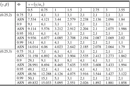
According to double sampling plan, the minimum sample sizes for 𝑛₁ and 𝑛₂ and ASN when = 0.75, 0.90, 0.95 and .99 and y ₀ =v=0.5, 0.75, 1.0, 1.5, 2.0, 2.75, 3.0 and 3.55 are shown in Tables (3.1- 3.3). As mentioned earlier, the parameter₀ is fixed at

Table 3.1: Minimum sample sizes and ASN for double sampling plans for GIW distribution with various values of the parameters γ and β

( )



,



 v=

(

y 0

)

0.5 0.75 1 1.5 2 2.75 3 3.55

(0.25,2) 0.75 7,1 4,1 3,1 3,1 2,1 2,1 2,1 2,1

ASN 7.534 4.121 3.44 2.579 2.238 2.136 2.096 1.84

0.9 9,1 6,1 3,1 3,1 2,1 2,1 2,1 2,1

ASN 9.114 5.576 3.212 2.912 2.204 2.1 2.075 1.986

0.95 10,1 6,1 4,1 3,1 2,1 2,1 2,1 2,1

ASN 9.936 6.077 4.085 2.708 2.194 2.087 2.069 2.02

0.99 14,1 6,1 4,1 3,1 2,1 2,1 2,1 1,1

ASN 14.014 6.06 4.023 2.642 2.185 2.078 2.064 1.79

(0.25,3) 0.75 31,1 7,1 6,1 4,1 3,1 2,1 2,1 2,1

ASN 31.158 6.892 6.363 3.904 2.535 2.412 2.273 1.862

0.9 29,1 9,1 8,1 8,1 4,1 4,1 3,1 1,1

ASN 28.991 8.694 8.465 7.635 3.935 3.608 3.433 1.994

0.95 49,1 12,1 4,1 4,1 4,1 4,1 3,1 3,1

ASN 48.56 12.288 4.126 4.075 3.916 3.544 3.427 3.122

0.99 50,1 15,1 5,1 3,1 2,1 2,1 2,1 2,1

ASN 49.832 15.033 5.095 2.551 2.026 1.892 1.881 1.858

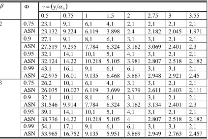
Table 3.2: Minimum sample sizes and ASN for double sampling plans for SGIW distribution with various values of the parameter β

  v=

(

y ₀

)

0.5 0.75 1 1.5 2 2.75 3 3.55

2 0.75 52,1 12,1 6,1 5,1 3,1 3,1 2,1 2,1

ASN 50.966 12.408 6.119 4.787 3.211 2.614 2.034 1.976

0.9 67,1 12,1 8,1 5,1 3,1 3,1 2,1 2,1

ASN 66.755 11.677 7.784 4.547 3.16 3.037 2.002 1.936

0.95 77,1 19,1 10,1 5,1 4,1 3,1 2,1 2,1

ASN 77.4 18.871 10.218 5.099 3.539 2.804 2.53 2.169

0.99 112,1 19,1 9,1 7,1 6,1 3,1 3,1 2,1

ASN 112.586 18.774 9.135 7.245 5.874 2.952 2.706 2.472

3 0.75 701,15 17,1 5,1 3,1 2,1 2,1 2,1 1,1

ASN 703.896 16.853 4.837 2.726 2.102 1.843 1.776 1.662

0.9 1380,22 21,1 7,1 5,1 2,1 2,1 2,1 2,1

ASN 1381 21.231 7.477 5.204 2.271 2.1 1.976 1.881

0.95 1245,28 24,1 6,1 3,1 3,1 2,1 2,1 2,1

ASN 1246 23.859 6.467 3.239 2.635 1.832 1.8 1.74

0.99 2106,37 34,1 9,1 4,1 2,1 2,1 2,1 2,1

Table 3.3: Minimum sample sizes and ASN for double sampling plans for CIR distribution with various values of the parameter β

  v=

(

y ₀

)

0.5 0.75 1 1.5 2 2.75 3 3.55

2 0.75 23,1 9,1 6,1 4,1 2,1 2,1 2,1 2,1

ASN 23.132 9.224 6.119 3.898 2.4 2.182 2.045 1.971

0.9 27,1 9,1 8,1 6,1 3,1 3,1 2,1 2,1

ASN 27.519 9.295 7.784 6.324 3.162 3.069 2.401 2.3

0.95 32,1 14,1 10,1 5,1 4,1 3,1 2,1 2,1

ASN 32.124 14.22 10.218 5.105 3.981 2.807 2.518 2.182

0.99 43,1 16,1 9,1 6,1 6,1 3,1 3,1 2,1

ASN 42.975 16.01 9.135 6.468 5.867 2.948 2.921 2.45

3 0.75 26,2 10,1 6,1 4,1 3,1 3,1 2,1 2,1

ASN 26.035 10.027 6.119 3.699 2.979 2.611 2.403 2.111

0.9 32,1 10,1 8,1 6,1 3,1 3,1 2,1 2,1

ASN 31.546 9.914 7.784 6.324 3.162 3.134 2.401 2.3

0.95 39,1 14,1 10,1 5,1 4,1 3,1 2,1 2,1

ASN 38.736 14.22 10.218 5.105 4 2.807 2.518 2.182

0.99 54,1 17,1 9,1 6,1 6,1 3,1 3,1 2,1

ASN 53.965 16.752 9.135 5.951 5.869 2.949 2.763 2.457

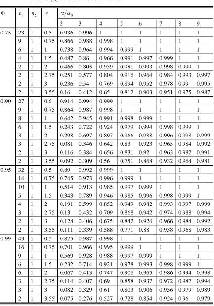
3.2 OC function based on double sampling

Once the minimum sample size 𝑛₁ and 𝑛₂ are obtained, one may be concerned to find the probability of acceptance the lot when the quality of an item is conforming enough. As mentioned previously, an item is considered to be conforming if the true median life to specified median life >1. The OC values according to (3.2) for different values of the median lifetime  _{0, consumer's confidence level}  and for given sampling plan

(

n1,n2,y 0

)

are shown in tables (3.4-3.6) for GIW, SGIW and CIR distributions when the parameter₀ =0.25 for the GIW distribution and ₀=2 for the three specified distributions.

3.3 The minimum ratios

The producer may be interested in knowing the minimum product quality level that will ensure the producer's risk, say 𝛿, at the specified level. For a given value 𝛿, the minimum ratio to ensure the producer's risk is less than or equal to 𝛿 = 0.05 can be obtained by satisfying the following inequality:

(

1−

)

n1

(

1+ ₁

(

1−

)

n2−1

)

0.95

n 

 (4.7)

respectively. The parameter ₀ = 0.25 for GIW distribution and the parameter ₀is studied at values 2 and 3 for three lifetime distributions.

Table 3.4: The OC values of acceptance sampling plan

(

n₁ ,n₂,c₁,c₂,v

)

for a given

 _with ₀ =0.25 and₀ =2 for GIW distribution

 n₁ n₂ v  ₀

2 3 4 5 6 7 8 9

0.75 7 1 0.5 0.99 1 1 1 1 1 1 1

4 1 0.75 0.799 0.997 1 1 1 1 1 1

3 1 1 0.478 0.931 0.998 1 1 1 1 1

3 1 1.5 0.2 0.609 0.895 0.984 0.999 1 1 1

2 1 2 0.083 0.323 0.634 0.858 0.96 0.992 0.999 1

2 1 2.75 0.036 0.15 0.348 0.575 0.767 0.892 0.957 0.986

2 1 3 0.025 0.108 0.269 0.475 0.673 0.823 0.917 0.966

2 1 3.55 0.029 0.104 0.233 0.399 0.572 0.723 0.838 0.913

0.90 9 1 0.5 0.986 1 1 1 1 1 1 1

6 1 0.75 0.694 0.994 1 1 1 1 1 1

3 1 1 0.514 0.939 0.998 1 1 1 1 1

3 1 1.5 0.149 0.551 0.873 0.98 0.998 1 1 1

2 1 2 0.088 0.332 0.642 0.862 0.961 0.992 0.999 1

2 1 2.75 0.039 0.157 0.358 0.584 0.773 0.895 0.959 0.986

2 1 3 0.026 0.111 0.273 0.479 0.677 0.826 0.918 0.967

2 1 3.55 0.019 0.078 0.193 0.353 0.529 0.69 0.815 0.9

0.95 10 1 0.5 0.984 1 1 1 1 1 1 1

6 1 0.75 0.659 0.993 1 1 1 1 1 1

4 1 1 0.388 0.909 0.997 1 1 1 1 1

3 1 1.5 0.179 0.586 0.886 0.983 0.998 0.998 1 1

2 1 2 0.09 0.335 0.645 0.863 0.962 0.962 0.999 1

2 1 2.75 0.04 0.159 0.361 0.587 0.775 0.775 0.959 0.986

2 1 3 0.026 0.112 0.275 0.481 0.678 0.678 0.919 0.967

2 1 3.55 0.017 0.074 0.186 0.344 0.52 0.52 0.81 0.897

0.99 14 1 0.5 0.97 1 1 1 1 1 1 1

6 1 0.75 0.661 0.993 1 1 1 1 1 1

4 1 1 0.396 0.911 0.997 1 1 1 1 1

3 1 1.5 0.189 0.598 0.891 0.983 0.998 1 1 1

2 1 2 0.091 0.338 0.647 0.864 0.962 0.992 0.999 1

2 1 2.75 0.041 0.161 0.363 0.589 0.776 0.897 0.959 0.986

2 1 3 0.026 0.113 0.276 0.482 0.679 0.827 0.919 0.967

Table 3.5: The OC values of acceptance sampling plan

(

n₁ ,n₂,c₁,c₂,v

)

for a given

 _with ₀ =2 for SGIW distribution



1

n n₂ v  0

2 3 4 5 6 7 8 9

0.75 52 1 0.5 1 1 1 1 1 1 1 1

12 1 0.75 0.996 1 1 1 1 1 1 1

6 1 1 0.933 1 1 1 1 1 1 1

5 1 1.5 0.462 0.954 0.999 1 1 1 1 1

3 1 2 0.277 0.782 0.976 0.999 1 1 1 1

3 1 2.75 0.135 0.484 0.813 0.958 0.994 0.999 1 1

2 1 3 0.204 0.535 0.814 0.949 0.99 0.999 1 1

2 1 3.55 0.129 0.381 0.662 0.859 0.955 0.989 0.998 1

0.90 67 1 0.5 1 1 1 1 1 1 1 1

12 1 0.75 0.996 1 1 1 1 1 1 1

8 1 1 0.9 1 1 1 1 1 1 1

5 1 1.5 0.488 0.958 0.999 1 1 1 1 1

3 1 2 0.297 0.794 0.977 0.999 1 1 1 1

3 1 2.75 0.07 0.371 0.745 0.939 0.991 0.999 1 1

2 1 3 0.212 0.545 0.819 0.95 0.99 0.999 1 1

2 1 3.55 0.14 0.398 0.675 0.866 0.957 0.989 0.998 1

0.95 77 1 0.5 1 1 1 1 1 1 1 1

19 1 0.75 0.991 1 1 1 1 1 1 1

10 1 1 0.848 1 1 1 1 1 1 1

5 1 1.5 0.43 0.949 0.999 1 1 1 1 1

4 1 2 0.242 0.759 0.972 0.999 1 1 1 1

3 1 2.75 0.111 0.448 0.793 0.953 0.993 0.999 1 1

2 1 3 0.105 0.401 0.733 0.921 0.984 0.999 1 1

2 1 3.55 0.091 0.319 0.61 0.832 0.945 0.989 0.997 1

0.99 112 1 0.5 1 1 1 1 1 1 1 1

19 1 0.75 0.991 1 1 1 1 1 1 1

9 1 1 0.872 1 1 1 1 1 1 1

7 1 1.5 0.256 0.91 0.998 1 1 1 1 1

6 1 2 0.067 0.559 0.936 0.997 1 1 1 1

3 1 2.75 0.095 0.422 0.777 0.949 0.993 0.999 1 1

3 1 3 0.085 0.366 0.708 0.912 0.982 0.997 1 1

Table 3.6: The OC values of acceptance sampling plan

(

n₁ ,n₂,c₁,c₂,v

)

for a given

 _with ₀ =2 for CIR distribution

 n₁ n₂ v  ₀

2 3 4 5 6 7 8 9

0.75 23 1 0.5 0.936 0.996 1 1 1 1 1 1

9 1 0.75 0.866 0.988 0.998 1 1 1 1 1

6 1 1 0.738 0.964 0.994 0.999 1 1 1 1

4 1 1.5 0.487 0.86 0.966 0.991 0.997 0.999 1 1

2 1 2 0.466 0.805 0.939 0.981 0.993 0.998 0.999 1

2 1 2.75 0.251 0.577 0.804 0.916 0.964 0.984 0.993 0.997

2 1 3 0.236 0.54 0.769 0.894 0.952 0.978 0.99 0.995

2 1 3.55 0.16 0.412 0.65 0.812 0.903 0.951 0.975 0.987

0.90 27 1 0.5 0.914 0.994 0.999 1 1 1 1 1

9 1 0.75 0.864 0.987 0.998 1 1 1 1 1

8 1 1 0.642 0.945 0.991 0.998 0.999 1 1 1

6 1 1.5 0.243 0.722 0.924 0.979 0.994 0.998 0.999 1

3 1 2 0.298 0.697 0.897 0.966 0.988 0.996 0.998 0.999

3 1 2.75 0.081 0.346 0.642 0.83 0.923 0.965 0.984 0.992

2 1 3 0.116 0.384 0.656 0.831 0.92 0.963 0.982 0.991

2 1 3.55 0.092 0.309 0.56 0.751 0.868 0.932 0.964 0.981

0.95 32 1 0.5 0.89 0.992 0.999 1 1 1 1 1

14 1 0.75 0.745 0.973 0.996 0.999 1 1 1 1

10 1 1 0.514 0.913 0.985 0.997 0.999 1 1 1

5 1 1.5 0.343 0.789 0.946 0.985 0.996 0.998 0.999 1

4 1 2 0.191 0.599 0.852 0.949 0.982 0.993 0.997 0.999

3 1 2.75 0.13 0.432 0.709 0.868 0.942 0.974 0.988 0.994

2 1 3 0.128 0.406 0.675 0.842 0.926 0.966 0.984 0.992

2 1 3.55 0.111 0.339 0.588 0.771 0.88 0.938 0.968 0.983

0.99 43 1 0.5 0.825 0.987 0.998 1 1 1 1 1

16 1 0.75 0.701 0.966 0.995 0.999 1 1 1 1

9 1 1 0.569 0.928 0.988 0.997 0.999 1 1 1

6 1 1.5 0.232 0.714 0.921 0.978 0.993 0.998 0.999 1

6 1 2 0.067 0.413 0.747 0.906 0.965 0.986 0.994 0.998

3 1 2.75 0.114 0.407 0.69 0.858 0.937 0.972 0.987 0.994

3 1 3 0.082 0.329 0.61 0.803 0.906 0.956 0.979 0.989

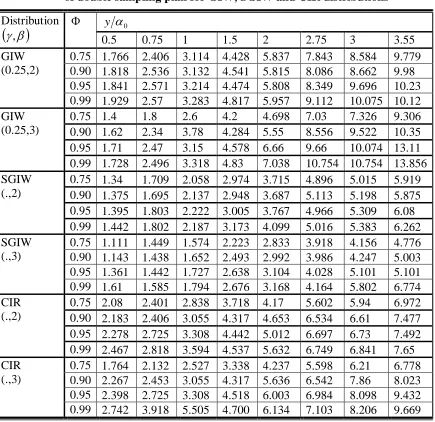
Table 3.7: Minimum true median to specified median ratio at producer's risk 0.05 of double sampling plan for GIW, SGIW and CIR distributions

Distribution

( )



,



 y ₀

0.5 0.75 1 1.5 2 2.75 3 3.55

GIW (0.25,2)

0.75 1.766 2.406 3.114 4.428 5.837 7.843 8.584 9.779 0.90 1.818 2.536 3.132 4.541 5.815 8.086 8.662 9.98 0.95 1.841 2.571 3.214 4.474 5.808 8.349 9.696 10.23 0.99 1.929 2.57 3.283 4.817 5.957 9.112 10.075 10.12 GIW

(0.25,3)

0.75 1.4 1.8 2.6 4.2 4.698 7.03 7.326 9.306

0.90 1.62 2.34 3.78 4.284 5.55 8.556 9.522 10.35

0.95 1.71 2.47 3.15 4.578 6.66 9.66 10.074 13.11

0.99 1.728 2.496 3.318 4.83 7.038 10.754 10.754 13.856 SGIW

(.,2)

0.75 1.34 1.709 2.058 2.974 3.715 4.896 5.015 5.919 0.90 1.375 1.695 2.137 2.948 3.687 5.113 5.198 5.875 0.95 1.395 1.803 2.222 3.005 3.767 4.966 5.309 6.08 0.99 1.442 1.802 2.187 3.173 4.099 5.016 5.383 6.262 SGIW

(.,3)

0.75 1.111 1.449 1.574 2.223 2.833 3.918 4.156 4.776 0.90 1.143 1.438 1.652 2.493 2.992 3.986 4.247 5.003 0.95 1.361 1.442 1.727 2.638 3.104 4.028 5.101 5.101 0.99 1.61 1.585 1.794 2.676 3.168 4.164 5.802 6.774 CIR

(.,2)

0.75 2.08 2.401 2.838 3.718 4.17 5.602 5.94 6.972

0.90 2.183 2.406 3.055 4.317 4.653 6.534 6.61 7.477 0.95 2.278 2.725 3.308 4.442 5.012 6.697 6.73 7.492 0.99 2.467 2.818 3.594 4.537 5.632 6.749 6.841 7.65 CIR

(.,3)

0.75 1.764 2.132 2.527 3.338 4.237 5.598 6.21 6.778 0.90 2.267 2.453 3.055 4.317 5.636 6.542 7.86 8.023 0.95 2.398 2.725 3.308 4.518 6.003 6.984 8.098 9.432 0.99 2.742 3.918 5.505 4.700 6.134 7.103 8.206 9.669

4. Description of Tables and An Illustrative Case

In this subsection, the numerical cases study for GIW(,,), SGIW(,,,) and CIR(,)

are introduced. The parameter ₀ is studied at value 0.25 for GIW distribution and the parameter ₀ is studied at values (2 and 3) for the three specified distributions which are presented in tables (3.1-3.7). The minimum sample sizes for the first and second samples ensure that the median life exceeds a given value 0,with various values of consumer's confidence level and corresponding acceptance limits c1 =0andc2 =1are showed in

tables (3.1-3.3). The operating characteristic values for the sampling plan

(

n₁,n₂,y ₀

)

with given various values of  and when-are determined in tables (3.4 c₂=1and c₁=0

Now, let ₀ =0.25 and ₀ =2 . Suppose Y₁,Y₂andY₃ be three lifetime of a product follows GIW, SGIW and CIR with shape parameters 0 =0.25 and 0 =2 corresponding to the equations (2.1), (2.9) and (2.10) respectively. Assume that a manufacturer decides to establish that true median life is at least 1000 hours with consumer's confidence level =0.99. The tester decides to stop the experiment at

750

0 =

y hours. Then, for acceptance limits c₁=0 and c₂=1, we have:

i. The GIW distribution: from table (6.1), the sample sizes n₁ =6 and n₂ =1.

ii. TheSGIW distribution: from table (6.2), the sample sizes n1=19and n2=1.

iii. TheCIR distribution: from table (6.3), the sample sizes n1 =16 and n2 =1.

Thus, for three lifetime distributions, 6, 19 and 16 units respectively have to be put on test for 750 hours. The lot is accepted if zero non-conforming item is recorded during the experiment and rejected if two or more non-conforming units are found. If exactly one non-conforming unit is found draw another sample for three distributions and put them on the same test. Accept the lot if a total of non-conforming units are one or fewer are recorded otherwise reject the lot. It is observed that the minimum sample sizes increase quickly as the shape parameter increases when the termination time ratio is short for GIW, SGIW and CIR distributions.

For zero and one failure scheme, the sampling plans for the GIW, SGIW and CIR distributions are respectively as(n₁=6 ,n₂=1, y₀=0.75), (n₁=18 ,n₂ =1, y₀=0.75), and (n₁=16 ,n₂=1, y₀=0.75). The OC values with =0.99 from Tables (3.4), (3.5) and (3.6)

can be tabulated as follows:

0



 2 3 4 5 6 7 8 9

OCGIW 0.661 0.992 1 1 1 1 1 1

OCSGIW 0.991 1 1 1 1 1 1 1

OCCIR 0.701 0.966 0.995 0.999 1 1 1 1

This means, the lot is accepted with probabilities 0.661, 0.991 and 0.701 for GIW, SGIW and CIR distributions respectively if the true median life of the units in the lot is twice than the specified median life. For three distributions, the probability of accepting the lot increases up to "one" if the true median life is 6 times than the specified median life. Also, the producer's risk for GIW, SGIW and CIR distributions will be 0.339, 0.009 and 0.299 respectively. To know the ratio corresponding to the producer’s risk of 0.05, can be found from the cumulative Table (3.7). For example, when the lifetime of product follows GIW, SGIW or CIR distributions, the minimum ratios  0 are 2.57, 1.802 and 2.818 respectively. In addition, the minimum ratios decrease as the shape parameters increases.

5. ConcludingRemarks

the lots was proposed. It was concluded that the SGIW is better distribution for fitting these plans compared to GIW and CIR distribution in spite of the sample size is larger for SGIW than the GIW and CIR distributions.

Acknowledgements

The authors would like to express their sincere gratitude to the anonymous the editor, the associate editor, and the referees for a careful checking of the details and for helpful comments and suggestions that improved this study.

References

1. Aslam, M. and Jun, C.-H. (2010), ‘‘A double acceptance sampling plan for generalized log-logistic distribution with known shape parameters’’. Journal of

Applied Statistics, 37(3), 405-414.

2. Aslam, M. Jun, C.-H. and Ahmed, M. (2010a). Design of a time-truncated double sampling plan for a general life distribution. Journal of Applied Statistics, 37, 8, 1369-1379.

3. Aslam, M., Kundu, D. and Ahmed, M. (2010b). Time truncated acceptance sampling plans for generalized exponential distribution. Journal of Applied

Statistics, 37, 4, 555-566.

4. Balakrishnan, N., Lieiva, V. and López, J. (2007). Acceptance sampling plans from truncated life tests based on the generalized Birnbaum-Saunders distribution. Communications in Statistics-Simulation and Computation, 36, 643-656.

5. Balamurali, S. Park, H., Jun, C.-H., Kim, K. and Lee, J. (2005), ‘‘Designing of variables repetitive group sampling plan involving minimum average sample number’’ Communication in Statistics-Simulation and Computation, 34(3), 799-809.

6. de Gusmão, F.R.S., Ortega E.M.M. and Corderio G.M. (2009). The Generalized Inverse Weibull distribution. Statistical Papers, pp. 591–619

7. Epstein, B. (1954) ‘‘Truncated life tests in the exponential case’’. Annals of

Mathematical Statistics, 25, 555-564.

8. Goode, H.P. and Kao, J.H.K. (1961). Sampling plans based on the Weibull disattribution. Proceedings of Seventh National Symposium on Reliability and

Quality Control. Philadelphia, Pennsylvania, 24-40.

9. Gupta, S.S. (1962). Life test sampling plans for normal and lognormal distributions. Technometrics, 4(2): 151-175.

10. Gupta, S.S. and Groll, P.A. (1961). Gamma distribution in acceptance sampling based on life test. Journal of the American Statistical Association, 56, 296, 942-970.

11. Jun, C.-H., Balamurali, S. and Lee, S.-H. (2006), ‘‘Variable sampling plans for Weibull distributed lifetimes under sudden death testing’’. IEEE Transactions on

12. Kantam, R.R.L. and Rosaiah, K. (1998). Half logistic distribution in acceptance sampling based on life tests. IAPQR Transactions, 23, 2: 117-125.

13. Mahdy, M. and Ahmed, B. (2016). Skew-generalized inverse weibull distribution its properties. Pakistan Journal statistic, 32(5), 329-348.

14. Montgomery, D.C. (2009), ‘‘Introduction to Statistical Quality Control ’’, 6th Edition, Jon Wiley & Sons, Inc., New York.

15. Muthulakshmi, S. and Selvi, B.G.G. (2013), ‘‘Double sampling plan for truncated life test based on Kumaraswamy log-logistic distribution’’. IOSR Journal of

Mathematics, 7(4), 29-37.