Atmos. Meas. Tech., 7, 95–105, 2014 www.atmos-meas-tech.net/7/95/2014/ doi:10.5194/amt-7-95-2014
© Author(s) 2014. CC Attribution 3.0 License.
Atmospheric
Measurement
Techniques
Open Access
A fast and easy-to-implement inversion algorithm for mobility
particle size spectrometers considering particle number size
distribution information outside of the detection range
S. Pfeifer1, W. Birmili1, A. Schladitz1,2, T. Müller1, A. Nowak1,3, and A. Wiedensohler1 1Leibniz Institute for Tropospheric Research, Permoserstraße 15, 04318 Leipzig, Germany
2Saxon State Office for Environment, Agriculture and Geology, Pillnitzer Platz 3, 01326 Dresden, Germany 3Physikalisch-Technische Bundesanstalt, Bundesallee 100, 38116 Braunschweig, Germany
Correspondence to: S. Pfeifer ([email protected])
Received: 19 April 2013 – Published in Atmos. Meas. Tech. Discuss.: 29 May 2013 Revised: 19 September 2013 – Accepted: 2 December 2013 – Published: 14 January 2014
Abstract. Multiple-charge inversion is an essential proce-dure to convert the raw mobility distributions recorded by mobility particle size spectrometers, such as the DMPS or SMPS (differential or scanning mobility particle sizers), into true particle number size distributions. In this work, we present a fast and easy-to-implement multiple-charge inver-sion algorithm with sufficient preciinver-sion for atmospheric con-ditions, but extended functionality. The algorithm can incor-porate size distribution information from sensors that mea-sure beyond the upper sizing limit of the mobility spectrom-eter, such as an aerodynamic particle sizer (APS) or an op-tical particle counter (OPC). This feature can considerably improve the multiple-charge inversion result in the upper size range of the mobility spectrometer, for example, when sub-stantial numbers of coarse particles are present. The program also yields a continuous size distribution from both sensors as an output. The algorithm is able to calculate the propaga-tion of measurement errors, such as those based on counting statistics, into on the final particle number size distribution. As an additional aspect, the algorithm can perform all in-version steps under the assumption of non-spherical particle shape, including constant or size-dependent shape factors.
1 Introduction
Mobility particle size spectrometers are widely used in aerosol science and have enjoyed broad application in both laboratory and field studies (Knutson and Whitby, 1975; Kousaka et al., 1985; McMurry, 2000). Rather than a true
particle number size distribution, they measure an electrical particle mobility distribution. Knowing the bipolar charge distribution (Wiedensohler, 1988) and the instrument re-sponses of the differential mobility analyser (DMA) and the particle counter or condensation particle counter (CPC), it is possible to convey the electrical particle mobility distri-bution into the true particle number size distridistri-bution. This procedure has been called multiple-charge inversion (Alofs and Balakumar, 1982; Kandlikar and Ramachandran, 1999). Surprisingly few publications are available that specify their algorithm in detail or the occupation of the matrix (e.g. Brun-ner, 2007). Wiedensohler et al. (2012) highlighted the need to characterize the performance of multiple-charge inversion routines as part of an attempt to enhance the mutual compa-rability of worldwide atmospheric aerosol measurements. In their work, 12 contemporary multiple-charge inversion rou-tines showed deviations of up to 5 % with respect to the re-sulting particle number concentration. The deviations were attributed, among others things, to different physical con-stants and charging probabilities used, different solutions to the matrix inversion problem, and different approaches of how to discretize, pre-process and post-process the data.
Only few of such inversion routines have been designed to handle size distribution information from multiple sen-sors. Some of our previous work highlighted, for example, the need to complement sub-micrometre mobility spectrom-eter information by additional super-micrometre size distri-bution measurements in specific atmospheric situations, such as dust plumes (Birmili et al., 2008; Schladitz et al., 2009). A lack of super-micrometre size distribution information could
96 S. Pfeifer et al.: Fast and easy-to-implement multiple-charge inversion algorithm
then lead to a drastic overestimation of the particle number size distribution in the upper size range of the mobility spec-trometer. In practice, the implementation of integrative inver-sion routines will closely depend on the type of available in-strumental parameters. Fiebig et al. (2005), for example, pro-posed an iterative method that is able to merge information from multiple size-selective instruments involving a differ-ential mobility analyser. Last but not least, it might be of ad-ditional benefit for an inversion routine to be compact and be able to easily process raw data during real-time data acquisi-tion, as well as large amounts of data during post-processing. In this work, we present the theoretical framework of a new inversion algorithm that inverts electrical particle mo-bility distribution from a momo-bility particle size spectrome-ter in conjunction with data from an aerodynamic particle sizer (APS) or an optical particle counter (OPC). The algo-rithm is designed for a maximum speed, while trying to re-main as accurate as possible with a minimum of assumptions. The framework allows for handling of non-spherical parti-cles, with particle shape being represented either by a con-stant shape factor or a size-dependent shape factor profile. A key feature of the algorithm is that we attempted to keep an analytical solution of the multiple-charge inversion problem, thus avoiding numerical iteration, which is possible at the expense of some accuracy as well as noise reduction. This is a distinction, for example, from other algorithms that apply external constraints such as non-negativity and smoothness (e.g. Talukdar and Swihart, 2003).
Due to the underlying strict system of linear equations, we are further able to compute how measurement errors, such as those based on counting statistics, propagate into the final particle number size distribution. The new capabilities of the algorithm are illustrated for two example cases.
2 Theory
The measured electrical particle mobility distribution (EPMD)f∗can be written as a convolution integral of the real particle number size distribution (PNSD) f and the transfer functionhwith the electrical particle mobilityZ as independent variable.1
f∗(Z)=(f∗h)(Z)= ∞ Z
−∞
f (Z0)h(Z−Z0)dZ0. (1)
It is possible to calculate the PNSD from the measured EPMD by deconvolution. From the beginning, we abandon the attempt to find the direct analytic solution of the transfer function for a deconvolution. The measured EPMD is given at N discrete mobility sampling points, so the problem is transformed to a system of equations which is easy to solve: 1A diameterDscaledxaxis is also possible, but is not used in
this work.
f1∗ .. . fN∗
=
a11 . . . a1N
..
. . .. ... aN1. . . aN N
f1 .. . fN
. (2)
Since we intend to consider non spherical particles in the algorithm, we employ the volume-equivalent particle diame-terDpveas the size parameter.
However, the DMA selects particles according to their electrical mobility
Z= n qe 3π η
Cc(Dpm) Dpm
, (3)
whereDpmis the mobility diameter andCCis the Cunning-ham correction factor. Often, the EPMD is already logged as particle mobility diameter for singly charged particles (Wiedensohler et al., 2012). These grid points can be recalcu-lated to volume-equivalent diameter using the transformation formula
Dpm Cc(Dpm)
=χ (Dpve) Dpve Cc(Dpve)
, (4)
whereχ (Dpve)is the size-dependent aerodynamic shape fac-tor, defined as the ratio of the drag of the arbitrarily shaped particle and the volume-equivalent sphere, in the Stokes regime. Examples of shape factors of real particles are pro-vided, for example, in Hinds (1999, p. 52).
2.1 DMA transfer function
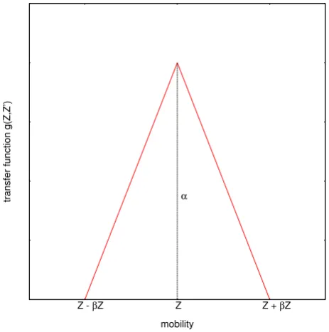
The transfer functiong(Z, Z0)of particles through a DMA at the positionZcan be simply described by a triangular func-tion with the heightα(Z)and the dimensionless half-width β(Z)or the dimensionless areaA(Z)=α(Z)β(Z). The size dependency ensures a consideration of diffusional broaden-ing of this transfer function (Birmili et al., 1997).
Ignoring multiply charged particles, as well as the count-ing efficiency of the CPC, the concentration downstream the DMA is given by the integral
c(Z)= ∞ Z
−∞ dc dZ0(Z
0
)g(Z, Z0)dZ0, (5)
while the transfer function (see Fig. 1) is given by Knutson and Whitby (1975):
g(Z, Z0)=
(α 2β
Z0
Z−(1+β) +
Z0
Z−(1−β) −2
Z0
Z−1
Z0∈((1−β)Z, (1+β)Z)
0 otherwise . (6)
S. Pfeifer et al.: Fast and easy-to-implement multiple-charge inversion algorithm 97
Sascha Pfeifer: Fast and easy-to-implement multiple charge inversion algorithm
9
transfer function g(Z,Z’)
mobility
α
Z
Z - βZ Z + βZ
Fig. 31: Schematic of a triangular DMA transfer function
Table 31: fit parameter for specific charge of the fifth degree
polynomial approximation of Wiedensohler (1988)
N
ai(N) -2 -1 0 +1 +2
a0 −26.3328 −2.3197 −0.0003 −2.3484 −44.4756
a1 35.9044 0.6175 −0.1014 0.6044 79.3772
a2 −21.4608 0.6201 0.3073 0.4800 62.8900
a3 7.0867 −0.1105 −0.3372 0.0013 26.4492
a4 −1.3088 −0.1260 0.1023 −0.1553 −5.7480
a5 0.1051 0.0297 −0.0105 0.0320 0.5059
Technology, 37, 145–161, 2003.
Wiedensohler, A.: an approximation of the bipolar charge distribu-tion for particles in the sub micron size range, Journal of Aerosol Science, 19, 387–389, 1988.
550
Wiedensohler, A., Birmilli, W., Nowak, A., Sonntag, A., Weinhold, K., and et al.: Mobility particle size spectrometers: harmoniza-tion of technical standards and data structure to facilitate high quality long-term observations of atmospheric particle number size distributions, Atmospheric Measurements and Technics, 5,
555
657–685, 2012.
0.0e+00 5.0e+03 1.0e+04 1.5e+04 2.0e+04
dc/dlogD
p
[cm
-3]
IFT ULUND ISAC NILU UHEL JRC PSI LAMP
0.90 0.95 1.00 1.05 1.10
10 100
5 50 500
rel. deviation to IFT
Dp [nm]
Fig. 32: Comparison of the performance of eight different
multiple charge inversion routines. Shown are the
differ-ent resulting PNSDs based on the very same EPMD, and
their relative deviation to the new inversion routine.
Repro-duced from Wiedensohler et al. (2012) (IFT - Leibniz
Insti-tute for Tropospheric Research, Leipzig, Germany; ULUND
- Lund University, Lund, Sweden; ISAC - Institute of
Atmo-spheric Sciences and Climate, Bologna, Italy; NILU -
Nor-wegian Institute for Air Research, Kjeller, Norway; UHEL
- University of Helsinki, Helsinki, Finland; JRC - Joint
Re-search Centre, Ispra, Italy; PSI - Paul Scherrer Institute,
Vil-ligen, Switzerland; LAMP - Laboratoire de M´et´eorologie
Physique, Clermont-Ferrand, France
0 1 2 3 4 5 6
0.01 0.1 1 10
raw particle number size distribution [cm
-3]
mobility equivalent diameter [µm]
raw electrical particle mobility distribution
Fig. 3a: raw electrical particle mobility distribution (EPMD)
in plain concentration
Fig. 1. Schematic of a triangular DMA transfer function
c(Z)'dc/dlnZ(Z)A(Z). With a conversion factorCi (see
Appendix A) we obtain the same approximation for the com-mon unit dc/dlogD. Considering also the CPC counting ef-ficiencyEC, we can find an expression for the DMA transfer
function using this approximation: hdma(Z−Z0)=
EC(Dpve(Z))A(Z)Ci(Dpve(Z))δ(Z0−Z), (7) whereδ is the Dirac delta function. It should be mentioned that, under conditions of atmospheric aerosol particles, the approximation is adequate due to weak variations of the PNSD in the range of the transfer function. For narrow par-ticle size distributions, such as those generated in the labo-ratory, this approximation is expected to be invalid. For such conditions, it is necessary to consider also the real shape of the transfer function.
2.2 Charging probability and transfer function of multiply charged particles
As already mentioned, we employ the volume-equivalent particle diameterDpveas the size parameter.
However, previous studies have shown that the bipolar dif-fusion charging for moderate non-spherical particles is sim-ilar to a sphere with the same mobility (Rogak and Fla-gan, 1992). Hence we use the mobility equivalent diameter Dpmas the size input to calculate the probability of multiply charged particles in a bipolar charge equilibrium. For strong non-spherical particles, for example particles with large as-pect ratios, this approach seems to be invalid (Ku et al., 2011).
Table 1. Fit parameter for specific charge of the fifth-degree
poly-nomial approximation of Wiedensohler (1988).
N
ai(N ) −2 −1 0 +1 +2
a0 −26.3328 −2.3197 −0.0003 −2.3484 −44.4756
a1 35.9044 0.6175 −0.1014 0.6044 79.3772
a2 −21.4608 0.6201 0.3073 0.4800 62.8900
a3 7.0867 −0.1105 −0.3372 0.0013 26.4492
a4 −1.3088 −0.1260 0.1023 −0.1553 −5.7480
a5 0.1051 0.0297 −0.0105 0.0320 0.5059
For singly and doubly charged particles smaller than 1 µm, we use the analytical approximation formula given by Wiedensohler (1988):
p(Dpm, n)=10
P5
i=0ai(n)
logDnmpmi
, (8)
whereai(n)are the fit parameters of the fifth-degree
polyno-mial approximation (see Table 1).
For larger particles or more highly charged particles we use the charge probability distribution by Gunn (1955):
p(Dpm, n)= 1 √
2π σexp
"
−(n−σln(0.875)) 2 2σ
#
σ =2π 0DpmkT qe2
. (9)
The measured EPMD is influenced by multiple charges; that is, for a given mobility diameter a mobility particle size spectrometer detects not only singly charged parti-cles with the electrical mobility Z but also larger, multi-ply charged particles with the same electrical mobilityZ/n (n=2,3, . . .), whereZ is the electrical mobility for singly charged particles, and also in the following sections.
Using Eqs. (8) and (9) we calculate the probability of spe-cific multiple charges p(Dpve, n). The transfer function to consider multiple chargeshchais
hcha(Z−Z0)=p
Dpm
1 1Z
, n=1
δ
Z0−1
1Z
+p
Dpm
1 2Z
, n=2
δ
Z0−1
2Z
+...
+p
Dpm
1
kZ
, n=k
δ
Z0−1
kZ
+...
=
∞
X
n=1
p
Dpm
1
nZ
, n
δ
Z0−1
nZ
. (10)
2.3 Resulting system of equations
The total transfer function h is the convolution of the DMA transfer function (Eq. 7) with the transfer function for
98 S. Pfeifer et al.: Fast and easy-to-implement multiple-charge inversion algorithm
Table 2. Symbol directory.
Symbol Explanation
Dpve particle diameter (volume equivalent)
Dpm particle diameter (mobility equivalent)
n number of charges
qe elementary charge
η dynamic viscosity
χ (Dpve) size-dependent aerodynamic shape factor
Z(Dpve, n) electrical particle mobility
α height of the DMA transfer function
β dimensionless width of DMA transfer func-tion
A dimensionless area of DMA transfer func-tion
f real particle number size distribution (PNSD)
f∗ measured electrical particle mobility distri-bution (EPMD)
p(Dp, n) charge probability
δ Dirac delta function
hdma approximated DMA transfer function,
con-sidering the transmission
hcha transfer function, considering the multiple
charges
h total transfer function
Ci(Dpve) conversion factor from dn/dlnZ to
dn/dlogD
A multiple-charge matrix
L transformation matrix, inverse of A
Lvar transformation matrix of variance
multiply charged particles (Eq. 10):
h(Z−Z0)= ∞ X
n=1 p
Dpm
1
nZ
, n
EC
Dpve
1
nZ
A
1
nZ
Ci
Dpve
1
nZ
δ
Z0−1 nZ
. (11)
LetEbe the value of efficiency by combining the proba-bility of multiply charged particles and the DMA efficiency inclusive the conversion factor with
E(Z, n)=p
Dpve
1
nZ
, n
EC
Dpve
1
nZ
A
1
nZ
Ci
Dpve
1
nZ
. (12)
As an example, in Appendix C, one can see the simple modification of the efficiencyEin the case of using a cloud condensation nuclei counter (CCNC) instead of a CPC. Fi-nally, we obtain an equation for the measured electrical parti-cle mobility distribution atZas a function of the real PNSD:
f∗(Z)= ∞ Z
−∞ f (Z0)
∞ X
n=1
E(Z, n)δ
Z0−1 nZ
dZ0
= ∞ X
n=1 E(Z, n)
∞ Z
−∞ f (Z0) δ
Z0−1 nZ
dZ0
= ∞ X
n=1
E(Z, n)f
1
nZ
. (13)
As previously mentioned, the measured EPMD is given in Ndiscrete mobility sampling points, where
fi∗=f∗(Zi)=
∞ X
n=1
E(Zi, n)f
1
nZi
. (14)
By using linear interpolation, given in Appendix B, we ob-tain
f
1
nZi
=
1
nZi−Zj
Zj+1−Zj
fj+1+
Zj+1−1nZi
Zj+1−Zj
fj
1
nZi ∈(Zj+1, Zj). (15) The sampling points of the real PNSD should be identi-cal to those of the measured EPMD. With this approach we are as close as possible to the actual information content of the measurement without additional assumptions. Thus we found a system of equations for the multiply charge inver-sion with the entries of matrix A:
aij =
∞ X
n=1
E(Zi, n)
1
nZi−Zj−1
Zj−Zj−1
1
nZi ∈ Zj, Zj−1
1 1nZi =Zj Zj+1−1nZi
Zj+1−Zj
1
nZi ∈ Zj+1, Zj
0 otherwise
, (16)
with
f∗=A·f. (17)
Because the number and position of the sampling points of the inverted PNSD and the measured EPMD should be identical, the matrix A is quadratic. Furthermore, due to i > j⇒aij =0, it is an upper triangular matrix, or a less
oc-cupied upper triangular matrix, which is easy to solve with a unique solution, e.g. using a simple Gauss–Jordan algorithm. Let L be the inverse of A. Finally, we obtain the solution as a system of equations:
f=A−1·f∗=L·f∗. (18) 2.4 Enhanced inversion
S. Pfeifer et al.: Fast and easy-to-implement multiple-charge inversion algorithm 99
inversion. One example is the presence of significant num-bers of coarse particles above the uppermost diameter chan-nel of the mobility particle size spectrometer. The reason is that multiply charged particles of that population will appear as particle counts that are superimposed onto the signal of particles with low charge (single and double) in the nominal mobility particle size spectrometer range.
Disturbances could only completely be avoided if a mobil-ity spectrometer were able to measure the PNSD across the entire range until the concentration reaches zero at the upper end. Due to technical reasons, however, the range of a mobil-ity particle size spectrometer cannot be extended far beyond 1–2 µm. In practice, the range of common mobility particle size spectrometers employed in atmospheric measurements terminates between 500 and 900 nm.
One approach has been to extrapolate the measured electri-cal particle mobility distribution into larger diameters (Brun-ner, 2007). This might be appropriate in the case of a con-tinuously decreasing number concentration towards larger particles, but usually not when a significant coarse particle mode is present. Therefore, information on larger particles is needed, for example, using an aerodynamic particle sizer (APS) or an optical particle counter (OPC). Schladitz et al. (2009) first proposed the approach of correcting the mea-sured EPMD for the effect of multiple charges prior to the actual inversion. We now present an implementation of this idea into the present inversion algorithm.
The real PNSD can be assumed to be a composition of a PNSDfmwithNsampling points, measured with a mobility particle size spectrometer, and an additional PNSD (volume-equivalent diameter)fa (in the following referred to as aP-NSD), e.g. measured with an optical or aerodynamic particle size spectrometer, withMsampling points.
f=
f1m .. . fNm fNa+1
.. . fNa+M
. (19)
The additional indicesmanda are added to indicate that the sampling points belong to the mobility particle size spec-trometer or the aPNSD. In accordance with Eq. (14) one can calculate the measured EPMD for the firstN sampling points, while the results for the aPNSD should be untouched by this algorithm:
fi∗= (P∞
n=1E(Zi, n)f
1
nZi
i≤N
f (Zi) i > N.
(20)
In case there is an overlap of the sampling points of both PNSDs, the function of the combined PNSD can be written
0.0e+00 5.0e+03 1.0e+04 1.5e+04 2.0e+04
dc/dlogD
p
[cm
-3]
IFT ULUND ISAC NILU UHEL JRC PSI LAMP
0.90 0.95 1.00 1.05 1.10
10 100
5 50 500
rel. deviation to IFT
Dp [nm]
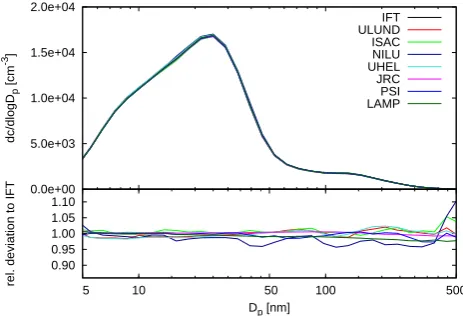
Fig. 2. Comparison of the performance of eight different
multiple-charge inversion routines. Shown are the different resulting PNSDs based on the very same EPMD and their relative deviation to the new inversion routine. Reproduced from Wiedensohler et al. (2012) (IFT – Leibniz Institute for Tropospheric Research, Leipzig, Ger-many; ULUND – Lund University, Lund, Sweden; ISAC – Institute of Atmospheric Sciences and Climate, Bologna, Italy; NILU – Nor-wegian Institute for Air Research, Kjeller, Norway; UHEL – Uni-versity of Helsinki, Helsinki, Finland; JRC – Joint Research Cen-tre, Ispra, Italy; PSI – Paul Scherrer Institute, Villigen, Switzerland; LAMP – Laboratoire de Météorologie Physique, Clermont-Ferrand, France.
as f
1
nZi
=
1 nZi−Zm
j
Zm j+1−Z
m j
fjm+1+Z
m j+1−
1 nZi
Zm j+1−Z
m j
fjm n1Zi∈(Zmj+1, Z m j)∧
1 nZi≥ZmN 1
nZi−Zja
Zaj+1−Z a j
fa j+1+
Zja+1− 1 nZi
Zaj+1−Z a j
fa j
1
nZi∈(Zaj+1, Zja) ∧ 1 nZi< ZNm
. (21)
In this case, the function values of the mobility particle size spectrometers are used as long as the multiply charged particles are in the detection range, or in other words, in the overlap range, we use the data of mobility particle spec-trometer.2It is important to assign it to the one or the other PNSD or a weighted value between both. If it is assigned completely to both, it would be overvalued and considered wrongly twice. This overlap is useful as an indicator. If the enhanced algorithm and the measurements are correct, the inverted PNSD of the mobility particle spectrometer and the aPNSD of the optical or aerodynamic particle size spectrom-eter fit together.
2Using the aPNSD in the overlap range is also possible, as well
as a weighted value between both
100 S. Pfeifer et al.: Fast and easy-to-implement multiple-charge inversion algorithm
Sascha Pfeifer: Fast and easy-to-implement multiple charge inversion algorithm 9
transfer function g(Z,Z’)
mobility α
Z
Z - βZ Z + βZ
Fig. 31: Schematic of a triangular DMA transfer function
Table 31: fit parameter for specific charge of the fifth degree polynomial approximation of Wiedensohler (1988)
N
ai(N) -2 -1 0 +1 +2
a0 −26.3328 −2.3197 −0.0003 −2.3484 −44.4756
a1 35.9044 0.6175 −0.1014 0.6044 79.3772
a2 −21.4608 0.6201 0.3073 0.4800 62.8900
a3 7.0867 −0.1105 −0.3372 0.0013 26.4492
a4 −1.3088 −0.1260 0.1023 −0.1553 −5.7480
a5 0.1051 0.0297 −0.0105 0.0320 0.5059
Technology, 37, 145–161, 2003.
Wiedensohler, A.: an approximation of the bipolar charge distribu-tion for particles in the sub micron size range, Journal of Aerosol Science, 19, 387–389, 1988.
550
Wiedensohler, A., Birmilli, W., Nowak, A., Sonntag, A., Weinhold, K., and et al.: Mobility particle size spectrometers: harmoniza-tion of technical standards and data structure to facilitate high quality long-term observations of atmospheric particle number size distributions, Atmospheric Measurements and Technics, 5,
555 657–685, 2012. 0.0e+00 5.0e+03 1.0e+04 1.5e+04 2.0e+04 dc/dlogD p [cm -3] IFT ULUND ISAC NILU UHEL JRC PSI LAMP 0.90 0.95 1.00 1.05 1.10 10 100
5 50 500
rel. deviation to IFT
Dp [nm]
Fig. 32: Comparison of the performance of eight different multiple charge inversion routines. Shown are the differ-ent resulting PNSDs based on the very same EPMD, and their relative deviation to the new inversion routine. Repro-duced from Wiedensohler et al. (2012) (IFT - Leibniz Insti-tute for Tropospheric Research, Leipzig, Germany; ULUND - Lund University, Lund, Sweden; ISAC - Institute of Atmo-spheric Sciences and Climate, Bologna, Italy; NILU - Nor-wegian Institute for Air Research, Kjeller, Norway; UHEL - University of Helsinki, Helsinki, Finland; JRC - Joint Re-search Centre, Ispra, Italy; PSI - Paul Scherrer Institute, Vil-ligen, Switzerland; LAMP - Laboratoire de M´et´eorologie Physique, Clermont-Ferrand, France
0 1 2 3 4 5 6
0.01 0.1 1 10
raw particle number size distribution [cm
-3]
mobility equivalent diameter [µm]
raw electrical particle mobility distribution
Fig. 3a: raw electrical particle mobility distribution (EPMD) in plain concentration
Fig. 3a. Raw electrical particle mobility distribution (EPMD) in
plain concentration.
The resulting matrix consists of four sub-parts:
aij=
aIij i≤N ∧ j ≤N aIIij i≤N ∧ j > N aIIIij i > N ∧ j≤N aIVij i > N ∧ j > N
. (22)
Under these conditions, there should be an overlap range and in this range the mobility particle size spectrometer data should be used; the first partaIij is identical to Eq. (16), de-scribing the interaction of the multiple charges of the PNSD with itself.
aijI = ∞ X
n=1
E(Zi, n)
1
nZi−Zjm−1
Zjm−Zjm−1
1
nZi ∈
Zmj, Zjm−1 1 1nZi =Zjm
Zm
j+1−
1
nZi
Zm
j+1−Zjm
1
nZi ∈
Zmj+1, Zjm
0 otherwise
. (23)
The second partaijII describes the interaction of multiply charged particles of the aPNSD and the PNSD measured with the mobility particle size spectrometer:
aijII= ∞ X
n=1
E(Zi, n)
1
nZai−Zj−1
Zaj−Zja−1
1
nZi∈
Zja, Zaj−1 ∧ 1
nZi< Z m N
1 1nZi=Zja ∧ n1Zi< ZNm Zja+1−1nZi
Zaj+1−Zja
1
nZi∈
Zja+1, Zja ∧ 1
nZi< Z m N
0 otherwise
, (24)
Generally, due to the side condition for the overlap size range, the first entries ofaIIijare empty (see Fig. 5b).
The last two parts are added to complete the rank of the matrix. Because the PNSD of the mobility particle size spec-trometer has no effect on the aPNSD,aijIII is a zero matrix:
10 Sascha Pfeifer: Fast and easy-to-implement multiple charge inversion algorithm
-200 -100 0 100 200 300 400 500 600
0.01 0.1 1 10
true particle number size distribution [cm
-3]
volume equivalent diameter [µm] conventional inversion
enhanced inversion APS
Fig. 3b: Results of the particle number size distribution (PNSD) obtained from multiple charge inversion with differ-ent degrees of functionality. Solid green line: aerodynamic particle size distribution (APS). Red dashed line: multiple charge inversion using only SMPS data. Red solid line: en-hanced multiple charge inversion combining APS and SMPS data. 0 500 1000 1500 2000 2500 3000 3500 4000 0 10 20 30 40 50 60
inverted PNSD [cm
-3]
raw PNSD [cm
-3] raw PNSD inverted PNSD 0 0.05 0.1 0.15
0.01 0.10 1.00
rel. std. dev.
vol. equivalent diameter [µm]
Fig. 4a: Example of the error propagation of a mobility par-ticle size spectrometer PNSD, Hohenpeissenberg, 23.02.12, one-hour average 0:00 - 1:00, EPMD (black) in plain con-centration (secondary y-axis) and PNSD (red). The fictive relative error of the results increases for sampling points in-fluenced by multiple charge correction from 10% to 15%
0 500 1000 1500 2000 2500 3000 3500 4000 0 10 20 30 40 50 60
inverted PNSD [cm
-3]
raw PNSD [cm
-3] raw PNSD inverted PNSD 0 0.1 0.2 0.3 0.4 0.5
0.01 0.10 1.00
rel. std. dev.
vol. equivalent diameter [µm]
Fig. 4b: Example of the error propagation of a mobility par-ticle size spectrometer PNSD, Hohenpeissenberg, 23.02.12, one-hour average 0:00 - 1:00, EPMD (black) in plain con-centration (secondary y-axis) and PNSD (red).. The relative error of the result is not significantly different from the input in case of Poisson counting statistic.
0 5 10 15 20
DMPS channel number 0
5
10
15
20
DMPS channel number
1.0e-07 1.0e-06 1.0e-05 1.0e-04 1.0e-03 1.0e-02 1.0e-01 1.0e+00
Fig. 5a: Visualization of the multiple charge matrix using only mobility particle size spectrometer data.
Fig. 3b. Results of the particle number size distribution (PNSD)
obtained from multiple-charge inversion with different degrees of functionality. Solid green line: aerodynamic particle size distribu-tion (APS). Red dashed line: multiple-charge inversion using only SMPS data. Red solid line: enhanced multiple-charge inversion combining APS and SMPS data.
aijIII=0 ∀ i, j. (25)
More precisely, as already mentioned, the aPNSD should be untouched, soaijIVis an identity matrix:
aijIV=1 ∀ i=j, (26)
A=
a11I . . . aI1N a1II(N+1) . . . a1II(N+M) ..
. . .. ... ... . .. ...
aIN1 . . . aIN N aIIN (N+1) . . . aIIN (N+M) a(NIII+1)1 . . . aIII(N+1)N a(NIV+1)(N+1) . . . a(NIV+1)(N+M)
..
. . .. ... ... . .. ...
a(NIII+M)1. . . aIII(N+M)Na(NIV+M)(N+1). . . a(NIV+M)(N+M) . (27)
By inserting the conditions to obtain the full rank, the ma-trix is A=
aI11 . . . a1IN a1II(N+1) . . . aII1(N+M) ..
. . .. ... ... . .. ... 0 . . . aN NI aN (NII +1) . . . aIIN (N+M) 0 . . . 0 1 . . . 0
..
. . .. ... ... . .. ... 0 . . . 0 0 . . . 1
. (28)
As the enhanced multiple-charge matrix is a sparsely oc-cupied upper triangular matrix, we are able to solve
f=L·f∗. (29)
S. Pfeifer et al.: Fast and easy-to-implement multiple-charge inversion algorithm 101
2.5 Error propagation
An important thing to investigate is the error propagation by using an inversion algorithm. As an assumption, let the measured EPMD be influenced by an error due to counting statistics of the condensation particle counter (CPC). Thus the values of the measured and inverted distributions can be interpreted as random variables. The expectation value of a linear transformationY of a random variableXis given by: E (Y )=E (aX+b)=aE (X)+b. (30)
Additionally, the sum ofnrandom variables Xi is given
by:
E
n
X
i=0 Xi
!
=
n
X
i=0
E (Xi) . (31)
As a result for the expectation value of the inverted PNSD we obtain
E(f)=L·E(f∗). (32)
The variance of the linear transformation is given by: Var(Y )=Var(aX+b)=a2Var(X) . (33)
In contrast to the expectation value, for the variance of the sum ofnrandom variablesXi, the condition that the random
variables are pairwise uncorrelated is required, i.e. statisti-cally independent. According to the Bienaymé formula, the variance is given by:
Var
n
X
i=0 Xi
!
=
n
X
i=0
Var(Xi) . (34)
Finally, for the variance of the inverted PNSD we obtain
Var(f)=Lvar·Var(f∗), (35)
where Lvaris a matrix occupied by the squared entries of L. lijvar=lij2 ∀ 0≥i, j≥N (36)
A similar expression exists for the resulting variance of theith sampling point, under the assumption that the random variables are correlated:
Var(fi)= N
X
j=1 lij
N
X
k=1
likCov(fj∗, f
∗
k), (37)
where Cov(fj∗, fk∗)is the covariance of thejth andkth sam-pling point of the EPMD.
These aspects are valid either for the conventional or the enhanced inversion.
0 500 1000 1500 2000 2500 3000 3500 4000
0 10 20 30 40 50 60
inverted PNSD [c
m
-3]
raw EPMD [c
m
-3]
raw EPMD inverted PNSD
0 0.05 0.1 0.15
0.01 0.10 1.00
rel. std. dev.
vol. equivalent diameter [µm]
(a)
0 500 1000 1500 2000 2500 3000 3500 4000
0 10 20 30 40 50 60
inverted PNSD [c
m
-3]
raw EPMD [c
m
-3] raw EPMD
inverted PNSD
0 0.1 0.2 0.3 0.4 0.5
0.01 0.10 1.00
rel. std. dev.
vol. equivalent diameter [µm] (b)
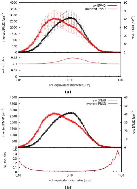
Fig. 4. Example of the error propagation of a mobility particle size
spectrometer PNSD, Hohenpeissenberg, 23 February 2012, 1 h av-erage 00:00–01:00 LT – EPMD (black) in plain concentration (sec-ondaryyaxis) and PNSD (red). (a) The fictive relative error of the results increases for sampling points influenced by multiple-charge correction from 10 to 15 %. (b) The relative error of the result is not significantly different from the input in the case of Poisson counting statistics.
3 Results
We devised a system of equations that directly transforms the measured EPMD to the real PNSD. This means an improve-ment in many respects.
1. The presented method preserves the original size bins of the measured electrical particle mobility distribu-tion. This avoids unnecessary interpolations of the data into new size bins and the typically associated changes in the originally measured information.
2. The operator matrix and its inverted matrix are based on linear equations. With matrix inversion accom-plished, the multiple-charge inversion problem reduces to a simple matrix multiplication, which is compu-tationally very efficient if multiple EPMDs with the same mobility bins should be processed.
102 S. Pfeifer et al.: Fast and easy-to-implement multiple-charge inversion algorithm
10
Sascha Pfeifer: Fast and easy-to-implement multiple charge inversion algorithm
-200 -100 0 100 200 300 400 500 600
0.01 0.1 1 10
true particle number size distribution [cm
-3]
volume equivalent diameter [µm] conventional inversion
enhanced inversion APS
Fig. 3b: Results of the particle number size distribution
(PNSD) obtained from multiple charge inversion with
differ-ent degrees of functionality. Solid green line: aerodynamic
particle size distribution (APS). Red dashed line: multiple
charge inversion using only SMPS data. Red solid line:
en-hanced multiple charge inversion combining APS and SMPS
data.
0 500 1000 1500 2000 2500 3000 3500 4000
0 10 20 30 40 50 60
inverted PNSD [cm
-3]
raw PNSD [cm
-3] raw PNSD
inverted PNSD
0 0.05 0.1 0.15
0.01 0.10 1.00
rel. std. dev.
vol. equivalent diameter [µm]
Fig. 4a: Example of the error propagation of a mobility
par-ticle size spectrometer PNSD, Hohenpeissenberg, 23.02.12,
one-hour average 0:00 - 1:00, EPMD (black) in plain
con-centration (secondary y-axis) and PNSD (red). The fictive
relative error of the results increases for sampling points
in-fluenced by multiple charge correction from 10% to 15%
0 500 1000 1500 2000 2500 3000 3500 4000
0 10 20 30 40 50 60
inverted PNSD [cm
-3]
raw PNSD [cm
-3] raw PNSD
inverted PNSD
0 0.1 0.2 0.3 0.4 0.5
0.01 0.10 1.00
rel. std. dev.
vol. equivalent diameter [µm]
Fig. 4b: Example of the error propagation of a mobility
par-ticle size spectrometer PNSD, Hohenpeissenberg, 23.02.12,
one-hour average 0:00 - 1:00, EPMD (black) in plain
con-centration (secondary y-axis) and PNSD (red).. The relative
error of the result is not significantly different from the input
in case of Poisson counting statistic.
0 5 10 15 20
DMPS channel number 0
5
10
15
20
DMPS channel number
1.0e-07 1.0e-06 1.0e-05 1.0e-04 1.0e-03 1.0e-02 1.0e-01 1.0e+00
Fig. 5a: Visualization of the multiple charge matrix using
only mobility particle size spectrometer data.
Fig. 5a. Visualization of the multiple-charge matrix using only
mo-bility particle size spectrometer data.
3. The algorithm can easily incorporate information from additional sensors measuring particles outside of the nominal measurement range of the particle mobility size spectrometer.
4. Because the inversion reduces to linear matrix multi-plication, computation of the effects of error propaga-tion is straightforward (see Sect. 2.5).
5. The algorithm can handle all procedures using a con-stant or size-dependent aerodynamic shape factor. 3.1 Validation of sub-micrometre EPMD inversion
We compared this inversion routine with many other inver-sion routines within the framework of technical harmoniza-tion of particle mobility size spectrometry (Wiedensohler et al., 2012). Figure 2 visualizes the bias of our inversion rou-tine against seven other contemporary inversion rourou-tines on the basis of an inversion of the same sub-micrometre EPMD. It can be seen that the different methods agree within a rel-ative deviation of 5 % for a wide particle size range. Larger deviations were explained by differing interpolation meth-ods.
3.2 Inversion of a wide size distribution combining SMPS and APS data
As already mentioned, particles outside of the measurement range of the mobility particle size spectrometer might affect the results of the sub-micrometre multiple-charge inversion. In Fig. 3a, we illustrate the benefits of a multiple-charge in-version combining information from multiple sizing instru-ments, involving SMPS and APS, for the case of an atmo-spheric dust storm event in Morocco (Schladitz et al., 2009).
Sascha Pfeifer: Fast and easy-to-implement multiple charge inversion algorithm
11
0 10 20 30 40 50 60 70 composed channel number
0
10
20
30
40
50
60
70
composed channel number
1.0e-07 1.0e-06 1.0e-05 1.0e-04 1.0e-03 1.0e-02 1.0e-01 1.0e+00
Fig. 5b: Visualization of the multiple charge matrix for the
enhanced case. The first quadrant corresponds to the matrix
entries shown in Fig. 5a. The second quadrant describes the
charge correction of the EPMD of the mobility particle size
spectrometer with information from additional sensors such
as an APS or OPC. The gap for the first entries of the second
quadrant is due to the finite overlap of both sizing sensors.
Table 32: Symbol directory
Symbol Explanation
Dpve particle diameter (volume equivalent)
Dpm particle diameter (mobility equivalent)
n number of charges
χ(Dpve) size dependent aerodynamic shape factor
Z(Dpve,n) electrical particle mobility
α height of the DMA transfer function
β dimensionless width of DMA transfer function
A dimensionless area of DMA transfer function
f real particle number size distribution (PNSD)
f∗ measured electrical particle mobility distribution (EPMD)
p(Dp,n) charge probability
δ dirac delta function
hdma approximated DMA transfer function, considering the transmission
hcha transfer function, considering the multiple charges
h total transfer function
Ci(Dpve) conversion factor fromdn/dlnZtodn/dlogD
A multiple charge matrix
L transformation matrix, inverse ofA
Lvar transformation matrix of variance
Fig. 5b. Visualization of the multiple-charge matrix for the
en-hanced case. The first quadrant corresponds to the matrix entries shown in Fig. 5a. The second quadrant describes the charge correc-tion of the EPMD of the mobility particle size spectrometer with information from additional sensors such as an APS or OPC. The gap for the first entries of the second quadrant is due to the finite overlap of both sizing sensors.
Figure 3b shows a bimodal shape of the EPMD, with num-ber concentration maxima around 80 and 300 nm. It is worth noting that in the uppermost SMPS sampling channel (corre-sponding to singly charged particles of 570 nm), the EPMD drops to just half of the maximum value of the EPMD. At the same time, the APS size distributions reveals the presence of a significant coarse particle mode with a volume-equivalent modal diameter around 700 nm. A multiple-charge inversion restricted to SMPS data will only necessarily need to inter-pret particle counts in the uppermost SMPS channel as singly charged particles. As can be seen in Fig. 3a, such an inversion causes an artificial depression in the final size distribution around 50–150 nm as a result of applying the multiple-charge inversion matrix. Also, the particle number size distribution at the upper tail of the distribution is heavily overestimated.
S. Pfeifer et al.: Fast and easy-to-implement multiple-charge inversion algorithm 103
dust based on the results of previous field studies (Schladitz et al., 2009).
3.3 Error propagation
The propagation of possible measurement errors from the EPMD into the final PNSD is illustrated in Fig. 4a and 4b. The basis is a 1 h average of ambient EPMD at the rural ob-servation site Hohenpeissenberg, Germany.
In Fig. 4a, we assume a fictive relative uncertainty (stan-dard deviation) of 10 % of particle number concentration measured in each channel of the EPMD. The error bars show the 95 % confidence interval under the assumption of a log-normal-distributed random variable. Particles smaller than 20 nm are only influenced by singly charged particles; there-fore the relative standard deviation is identical to the mea-sured data. In the range from 20 to 600 nm an increase of the error of the inverted PNSD is noticeable. In this case, the error cumulates up to 15 %. Sampling points larger than 600 nm are also influenced by multiple charges, and one would expect also an increase of the error, but these multi-ply charged particles are outside of the detection range of the mobility particle size spectrometer. From this it follows that the relative standard deviation is identical to the measured values.
The same effect occurs when analysing the Poisson statis-tics based on experimental particle number counts for each raw concentration channel (see Fig. 4b), but not as signif-icantly. The underlying reason is that the size range, influ-enced by multiply charged particles, exhibits the smallest er-rors, 1.3 % at minimum.
The idea of the analytical error propagation is expandable in the case of correlated sampling points. Errors or uncertain-ties for the diameters or thex values of the sampling points will influence the matrix elements. Therefore, it cannot be analysed in the same way. To investigate this effect, Monte Carlo simulations must be used further on.
3.4 Suggested improvements and extensions
Although the given algorithm represents a flexible tool, we see room for future improvements. A first issue would be the use of a uniform theory for the charging probability across the complete particle size range, especially for the enhanced inversion. A candidate would be the theory of Fuchs (1963). The interpolations leading to Eq. (15) (Sect. 2.3) could be achieved by higher polynomial interpolation methods, possi-bly spline interpolation, rather than by linear interpolation.
However, it must be noted that these methods have their own disadvantages, as they need proper initial and boundary conditions and might also lead to artificial overshooting and therefore to an amplification of noise. For a dense grid of sampling points the gain of accuracy does not seem to be in proportion to the numerical effort.
An issue that is in principle relevant is the true deconvo-lution of the DMA transfer function, whose finite width is ignored by the present version of the algorithm. Moreover, the width, area and shape of the DMA transfer function usu-ally depend on particle size, especiusu-ally for the highly dif-fusive particles in the lower range of mobility particle size spectrometers (Flagan, 1999). It is possible to calculate the analytic solution of convolution, or the integral, of a trian-gular or bell-shaped transfer function, especially under the assumption of a linearly interpolated PNSD, and then de-termine the occupation of the matrix. Implementing such features would make this algorithm usable for very narrow PNSD and possibly improve the results for the smaller di-ameter range. It needs to be mentioned, however, that the transfer matrix would become a band matrix with entries on both sides on the main diagonal. The solution of such an inversion is more sensitive to variations in the input data and leads to an amplification of experimental noise. To avoid such a behaviour, numerically more demanding algorithms using smoothing constrains would be required (e.g. Talukdar and Swihart, 2003). The actual advantages of our algorithm – minimum resource consumption and high computational speed at an acceptable accuracy for atmospheric measure-ments including error propagation calculations – would be diminished.
4 Conclusions
We have presented the mathematical description of a multiple-charge inversion algorithm for mobility particle size spectrometers which is based on a forward transformation of the particle number size distribution (PNSD). The algorithm is based on very few approximations and interpolations, sug-gesting a number of advantages. Avoiding the interpolation of electrical particle mobility distributions (EPMD) onto a new grid helps to conserve the original experimental infor-mation. Due to the strict linear nature of the system of equa-tions, the algorithm is extremely fast. Importantly, we en-countered no serious deviations to previous inversion rou-tines due to these simplifications.
Furthermore, the algorithm is able to balance a signal caused by multiply charged particles outside the nominal measurement range of a mobility particle size spectrome-ters by using additional information collected with optical or aerodynamic particle size spectrometers. This extended functionality was shown to be particularly relevant in atmo-spheres with numerous coarse particles, which could be re-suspended mineral dust or sea spray particles.
Finally, because of this strict linear dependency, it is pos-sible to calculate the error propagation, due to, for example, instrumental uncertainty or counting statistics in the inverted particle number size distribution. This is a frequently ignored aspect, but appears necessary to give the final particle num-ber size distribution a statistical confidence and precision.
104 S. Pfeifer et al.: Fast and easy-to-implement multiple-charge inversion algorithm
All aspects of the algorithm are applicable for non-spherical particles, with non-sphericity being handled through an aerodynamic particle shape factor that transforms mobility equivalent into volume-equivalent diameters. This issue is particularly relevant for the enhanced inversion us-ing information on super-micrometre dust particles.
Appendix A
Conversion of number size distribution
Transformation of dn/dlnZto dn/dlogD(dn/dlogDpve): dn
dlogDpve
=ln(10)Dpve Z
dZ dDpve
dn
dlnZ, (A1)
where Z= n qe
3π η
Cc(Dpve) χ (Dpve) Dpve
. (A2)
LetC be the conversion factor for the density transforma-tion:
C(Dpve)=ln(10) Dpve
Z
dZ dDpve
, (A3)
or the inverseCi(Dpve)=C(Dpve)−1, and as a result dn
dlnZ =Ci(Dpve) dn dlogDpve
. (A4)
Appendix B
Linear interpolation
The unknown real PNSD, the solution, is a continuous func-tion; therefore we assume a linear interpolation for the given number of sampling pointsN.
f (x)=
f10(x−x1)+f1 x1≤x≤x2 ..
. ...
fN0−1(x−xN−1)+fN−1 xN−1≤x≤xN
0 otherwise
,
(B1) with
fi=f (xi), fi0=
fi+1−fi
xi+1−xi
. (B2)
Forx∈(xi, xi+1)we obtain the function value f (x)= x−xi
xi+1−xi
fi+1+
xi+1−x xi+1−xi
fi. (B3)
Appendix C
Multiple-charge inversion with CCNC
Using a CPC, the EPMD is given by:
fi∗=f∗(Zi)=
∞ X
n=1
E(Zi, n)f
1
nZi
. (C1)
Using a CCNC instead of a CPC modifies the efficiency. In addition, we need the size-dependent activationa(D):
fCi∗ =f∗(Zi)=
∞ X
n=1
E(Zi, n)a
1
nZi
f
1
nZi
. (C2)
Witha
1
nZi
f
1
nZi
=fC
1
nZi
, we obtain
f∗C=A·fC, (C3)
wherefC is the real PNSD of the activated particles and
f∗Cis the measured EPMD when using a CCNC instead of a CPC.
Acknowledgements. We would like to thank J.-L. Jimenez for edit-ing, as well as the anonymous referees for their critical feedbacks.
Edited by: J.-L. Jimenez
References
Alofs, D. J. and Balakumar, P.: Inversion to obtain aerosol size dis-tributions from measurements with a differential mobility ana-lyzer, J. Aerosol Sci., 13, 513–527, 1982.
Birmili, W., Stratmann, F., Wiedensohler, A., Covert, D., Russel, L. M., and Berg, O.: Determination of differential mobility an-alyzer transfer functions using identical instruments in series, Aerosol Sci. Technol., 27, 215–223, 1997.
Birmili, W., Schepanski, K., Ansmann, A., Spindler, G., Tegen, I., Wehner, B., Nowak, A., Reimer, E., Mattis, I., Müller, K., Brüggemann, E., Gnauk, T., Herrmann, H., Wiedensohler, A., Althausen, D., Schladitz, A., Tuch, T., and Löschau, G.: A case of extreme particulate matter concentrations over Central Europe caused by dust emitted over the southern Ukraine, Atmos. Chem. Phys., 8, 997–1016, doi:10.5194/acp-8-997-2008, 2008. Brunner, J.: Particle measurements (size distribution and number)
with a SMPS – Technical basis and evaluation procedures (trans-lated from "Partikelmessungen (Grössenverteilung und Anzahl) mit einem SMPS – Grundlagen und Auswerteverfahren"), Tech. Rep. No. 20051105, Stadt Zürich, Umwelt- und Gesundheitss-chutz Zürich UGZ, 8021 Zürich, Revision 2.1, 2007.
Fiebig, M., Stein, C., Schröder, F., Feldpausch, P., and Petzold, A.: Inversion of data containing information on the aerosol particle size distribution using multiple instruments, J. Aerosol Sci., 36, 1353–1372, 2005.
S. Pfeifer et al.: Fast and easy-to-implement multiple-charge inversion algorithm 105
Fuchs, N. A.: On the stationary charge distribution on aerosol Par-ticles in a bipolar ionic atmosphere, Pure Appl. Geophys., 56, 185–193, 1963.
Gunn, R.: The statistical electrification of aerosols by ionic diffu-sion, J. Colloid Sci., 10, 107–119, 1955.
Hinds, W. C.: Aerosol Technology: Properties, Behavior, and Mea-surement of Airborne Particles, Wiley-Interscience, 2nd Edn., 1999.
Kandlikar, M. and Ramachandran, G.: Inverse methods for analysing aerosol spectrometer measurements: a critical review, J. Aerosol Sci., 30, 413–437, 1999.
Knutson, E. O. and Whitby, K. T.: Aerosol classification by electri-cal mobility apperatus, theory, and applications, J. Aerosol Sci., 6, 443–451, 1975.
Kousaka, Y., Okuyama, K., and Adachi, M.: Determination of par-ticle size distribution of ultra-fine aerosols using a differential mobility analyzer, Aerosol Sci. Technol., 4, 209–225, 1985. Ku, B. K., Deye, G. J., Kulkarni, P., and Baron, P. A.: Bipolar
diffu-sion charging of high-aspect ratio aerosols, J. Electrostatics, 69, 541–647, 2011.
McMurry, P. H.: A review of atmospheric aerosol measurements, Atmos. Environ., 34, 1959–1999, 2000.
Rogak, S. N. and Flagan, R. C.: Bipolar diffusion charging of spheres and agglomarated aerosol particles, J. Aerosol Sci., 23, 693–710, 1992.
Schladitz, A., Müller, T., Kaaden, N., Maasling, A., Kandler, K., Ebert, M., Weinbruch, S., Deutscher, C., and Wiedensohler, A.: In situ measurements of optical properties at Tinfou (Morocco) during the Saharan Mineral Dust Experiment SAMUM 2006, Tellus, 61B, 64–78, 2009.
Stratmann, F., Kauffeldt, T., Hummes, D., and Fissan, H.: Differen-tial electrical mobility analysis: A theoretical study, Aerosol Sci. Technol., 26, 368–383, 1997.
Talukdar, S. S. and Swihart, M. T.: An improved data inversion pro-gram for obtaining aerosol size distributions from scanning dif-ferential mobility analyzer data, Aerosol Sci. Technol., 37, 145– 161, 2003.
Wiedensohler, A.: An approximation of the bipolar charge distribu-tion for particles in the submicron size range, J. Aerosol Sci., 19, 387–389, 1988.
Wiedensohler, A., Birmili, W., Nowak, A., Sonntag, A., Weinhold, K., Merkel, M., Wehner, B., Tuch, T., Pfeifer, S., Fiebig, M., Fjäraa, A. M., Asmi, E., Sellegri, K., Depuy, R., Venzac, H., Vil-lani, P., Laj, P., Aalto, P., Ogren, J. A., Swietlicki, E., Williams, P., Roldin, P., Quincey, P., Hüglin, C., Fierz-Schmidhauser, R., Gysel, M., Weingartner, E., Riccobono, F., Santos, S., Grüning, C., Faloon, K., Beddows, D., Harrison, R., Monahan, C., Jen-nings, S. G., O’Dowd, C. D., Marinoni, A., Horn, H.-G., Keck, L., Jiang, J., Scheckman, J., McMurry, P. H., Deng, Z., Zhao, C. S., Moerman, M., Henzing, B., de Leeuw, G., Löschau, G., and Bastian, S.: Mobility particle size spectrometers: harmonization of technical standards and data structure to facilitate high qual-ity long-term observations of atmospheric particle number size distributions, Atmos. Meas. Tech., 5, 657–685, doi:10.5194/amt-5-657-2012, 2012.