Atmos. Meas. Tech., 6, 3563–3576, 2013 www.atmos-meas-tech.net/6/3563/2013/ doi:10.5194/amt-6-3563-2013
© Author(s) 2013. CC Attribution 3.0 License.
Atmospheric
Measurement
Techniques
Open Access
Implementation of a 3D-Var system for atmospheric profiling data
assimilation into the RAMS model: initial results
S. Federico
ISAC-CNR, UOS of Rome, Rome (RM), Italy
Correspondence to: S. Federico ([email protected])
Received: 3 March 2013 – Published in Atmos. Meas. Tech. Discuss.: 12 April 2013
Revised: 14 November 2013 – Accepted: 14 November 2013 – Published: 17 December 2013
Abstract. This paper presents the current status of devel-opment of a three-dimensional variational data assimilation system (3D-Var). The system can be used with different nu-merical weather prediction models, but it is mainly designed to be coupled with the Regional Atmospheric Modelling Sys-tem (RAMS). Analyses are given for the following param-eters: zonal and meridional wind components, temperature, relative humidity, and geopotential height.
Important features of the data assimilation system are the use of incremental formulation of the cost function, and the representation of the background error by recursive filters and the eigenmodes of the vertical component of the back-ground error covariance matrix. This matrix is estimated by the National Meteorological Center (NMC) method.
The data assimilation and forecasting system is applied to the real context of atmospheric profiling data assimilation, and in particular to the short-term wind prediction. The anal-yses are produced at 20 km horizontal resolution over central Europe and extend over the whole troposphere. Assimilated data are vertical soundings of wind, temperature, and rela-tive humidity from radiosondes, and wind measurements of the European wind profiler network.
Results show the validity of the analyses because they are closer to the observations (lower root mean square error (RMSE)) compared to the background (higher RMSE), and the differences of the RMSEs are in agreement with the data assimilation settings.
To quantify the impact of improved initial conditions on the short-term forecast, the analyses are used as initial con-ditions of three-hours forecasts of the RAMS model. In par-ticular two sets of forecasts are produced: (a) the first uses the ECMWF analysis/forecast cycle as initial and boundary conditions; (b) the second uses the analyses produced by the
3D-Var as initial conditions, then it is driven by the ECMWF forecast.
The improvement is quantified by considering the horizon-tal components of the wind, which are measured at asynop-tic times by the European wind profiler network. The results show that the RMSE is effectively reduced at the short range. The results are in agreement with the set-up of the numerical experiment.
1 Introduction
Modern numerical weather prediction (NWP) data assimi-lation systems use information from a range of sources to provide the best estimate of the atmospheric state (i.e. the analysis) at a given time. These systems combine informa-tion coming from the observainforma-tions, an a priori estimate of the atmospheric state (the background or first-guess field), detailed error statistics, and the law of physics.
Nowadays, increased computing power coupled with greater access to real-time a-synoptic data is paving the way toward a new generation of high-resolution (10 km or less in the horizontal plane) operational mesoscale analysis and forecasting systems (Zou et al., 1995; Sun and Crook, 1997; Lazarus et al., 2002; Kalnay, 2003; Barker et al., 2004; Zu-panski et al., 2005; Huang et al., 2009). Moreover, better ini-tial conditions are increasingly considered as of the utmost importance for a range of NWP applications, in particular at the short range (0–12 h, Zhang et al., 2005; Schenkman et al., 2011; Sun et al., 2012; Wang et al., 2013; Sun and Wang, 2013).
3564 S. Federico: Implementation of a 3D-Var system
standard atmospheric variables, such as radiances, and they include the imposition of dynamic balance either by the model itself (4D-Var) or through the explicit use of balance equations. In recent years, these advantages have fostered the implementation of variational data assimilation systems in limited area models (Zou et al., 1995; Barker et al., 2004; Huang et al., 2009; Zupanski et al., 2005). These systems replaced previously used schemes such as optimal interpola-tion (Parrish and Derber, 1992; Rabier et al., 2000).
This paper shows the development of a three-dimensional stand-alone data assimilation system tailored for the Re-gional Atmospheric Modeling System (RAMS; Cotton et al., 2003; Pielke, 2002). In particular, the data assimilation sys-tem can use the RAMS fields as background and the analyses can be used to initialize the RAMS model (cycling mode).
The analysis system uses the incremental formulation of the cost function (Courtier et al., 1994), which reduces the computational cost, and a control variable transform to make the minimization of the cost function practicable.
This paper shows an upgrade of the 2D-Var data assim-ilation system reported by Federico (2013). Two important features were introduced: (a) the use of the 3D-Var method, which replaces the 2D-Var; (b) the option to run the anal-ysis on the same horizontal coordinate system as RAMS, which simplifies the interaction between the data assimila-tion scheme and the meteorological model.
It is important to mention that a 4D-Var data assimila-tion system is already in use for RAMS, designed as RAM-DAS (Regional Atmospheric Modeling and Data Assimila-tion System; Zupanski et al., 2005; Polkinghorne et al., 2010; Polkinghorne and Vukicevic, 2011). Nevertheless, there are two main reasons, practical and scientific, for implementing the 3D-Var system of this paper:
1. The RAMDAS system uses the RAMS model and its adjoint but it is not part of the RAMS model suite. RAMS comes with other data assimilation sys-tems, such as nudging or dynamical adaptation (Pielke, 2002), but without a variational data assimilation sys-tem. This work aims to fill this void by realizing a sim-ple but effective variational data assimilation system, suitable for applications and operational implementa-tion in small meteorological centres. The 3D-Var, in-deed, requires less computational resources compared to 4D-Var (Rabier et al., 2000) or ensemble Kalman filters (Anderson, 2001). Compared to the 4D-Var, it does not require the tangent linear and adjoint mod-els and is simpler to implement. Moreover, the 3D-Var can be effective at improving the initial model state and has the advantages of variational data assimilation systems.
2. To the knowledge of the author, the RAMDAS sys-tem was mainly developed and applied at the cloud-resolving scales, while the 3D-Var system of this pa-per is designed for larger scales (synoptic, meso-α),
as emphasized by the model resolution adopted in this work and by the balance equations used in the 3D-Var.
As a consequence of the last point, there are also technical differences between RAMDAS and the 3D-Var, the most im-portant difference being that the 3D-Var uses the incremental formulation of the cost function differently from RAMDAS. The incremental formulation of the cost function was chosen because it reduces the computational cost and it improves the conditioning of the cost function because of the linearization required in its implementation. Even though the incremen-tal formulation of the cost function might not be suitable for convective-scales because of the linearization required in its formulation, recent studies show the applicability of this ap-proach to the convective scale for the WRF (Weather Re-search and Forecasting) model (Sun et al., 2012; Wang et al., 2013).
Another difference between the 3D-Var and RAMDAS is that the former uses the zonal and meridional wind compo-nents as control variables while RAMDAS uses the velocity potential and stream function. Using the velocity potential and stream function changes the subspace in which the cor-relations are calculated and allows for a simpler modelling of the covariances. This makes saves considerable computing time. Nevertheless, numerical investigations (Sun and Wang, 2013) have shown differences between the two choices that affect the final analysis. Because of this difference, the zonal and meridional wind components, which are prognostic vari-ables of RAMS, have been chosen as control varivari-ables in the 3D-Var system.
Another difference between the two data assimilation sys-tems, which is worth mentioning here, is the different rep-resentation of the background error covariance matrix. This matrix is directly modelled in RAMDAS as square root cor-relation matrices, while a control variable transform is used in the 3D-Var. The RAMDAS approach avoids the need for an eigenvalue–eigenvector decomposition, while the 3D-Var approach can be used to filter modes responsible for a (small) fraction of the error variance, thus requiring less computa-tional resources.
S. Federico: Implementation of a 3D-Var system 3565
The paper is divided as follows: Sect. 2 provides details about the data assimilation system; Sect. 3 shows the numer-ical experiment set-up; Sect. 4 gives the results of the ap-plication to the short-term wind forecast; and Sect. 5 gives conclusions.
2 The data assimilation system
The basic goal of the 3D-Var algorithm is to produce an op-timal estimate of the true atmospheric state at analysis time through iterative solution of a prescribed cost function (Ide et al., 1997):
J (x)=1 2(x−x
b)TB−1(x−xb)
+1 2 y
o−H (x)T
R−1 yo−H (x), (1)
whereJ (x)is the cost function,x is the state vector,xbis the background state,H is the forward observational oper-ator,yo is the vector of the observations, and B and R are the background and observational errors covariance matri-ces, respectively. The observational errors covariance matrix R is the sum of the covariance of instrumental errors matrix (E) and of the covariance of representativeness errors matrix (F), i.e R=E+F.
The problem can be summarized as the iterative solution of Eq. (1) to find the analysis statexathat minimizesJ (x). This solution represents the a posteriori maximum likelihood (minimum variance) estimate of the true state of the atmo-sphere given the two sources of a priori data: backgroundxb and observationsyo(Lorenc, 1986).
For a model statexwithn∼106–107degrees of freedom, the direct solution of Eq. (1) is practically unfeasible because it requires∼O(n2)calculations. One practical implementa-tion is to perform a precondiimplementa-tioning via a control variableν defined byx0=Uν, wherex0=x−xbis the model variable increment. The transform U is chosen to satisfy the relation-ship B=UUT. Using the incremental formulation (Courtier et al., 1994) and the control variable transform, Eq. (1) may be rewritten:
J=1 2ν
Tν+1
2
yo0−HUνTR−1yo0−HUν, (2) whereyo0=yo−H(xb) is the innovation vector and H is the linearization of the nonlinear observation operator H1. In this form, the background term is diagonalized, reducing the number of calculations required fromO(n2)toO(n).
The control variable ν is a vector ν=(u0,v0,RH0,T0), whereu0 andv0 are the zonal and meridional wind compo-nent increments,RH0is the relative humidity increment, and 1It is worth noting that the nonlinearity of the observation opera-tor H is considered in the computation of the innovation vecopera-toryo0. This is accomplished in the outer loop for variational methods using the incremental approach with an outer loop (Huang et al., 2009).
T0 is the temperature increment. The model variable
incre-mentx0is a vectorx0= (Z0,u0,v0,RH0,T0), whereZ0is the
geopotential height increment and the other symbols are as inν.
The transformx0=Uνfrom the control variableνto the model variable increment x0 is implemented through three operators, namelyUp,Uv, andUh, applied in sequence.
The transformUhis implemented through recursive filters (Purser et al., 2003; Barker et al., 2004). The recursive filter performs the task of convolving a spatial distribution of the analysis increments with a smoothing kernel, which is the covariance function of the background error. A single pass of a recursive filter consists of an initial advancing smoothing:
Fi =(1−α)Di+αFi−1 (3)
for increasing indexi, whereDis the input forcing andF is the result of the sweep, followed by a backing sweep
Ri =(1−α)Fi+αRi+1 (4)
for decreasingi, whereF is now the input andR is the re-sponse of the filter. The smoothing parameterαlies between 0 and 1 and determines the correlation length of the smooth-ing response function.
The single-pass recursive filter of the operatorUhinvolves one smoothing in the WE direction followed by one smooth-ing in the NS direction.
The recursive filter has two parameters: the number of passes and the length scaled. The number of passes deter-mines the response of the filter. In particular, forN=2 the response approximates a second-order auto-regressive func-tion (SOAR), while forN= ∞the response is Gaussian. In this paper twelve passes are used. This value ensures a well-shaped filter response, without the formation of unphysical lozenge-shaped model variable incrementsx0.
The length scales of the recursive filters, which determine the smoothing parameterα(see Barker et al., 2003 for the de-tails of the calculation) are computed by the National Meteo-rological Center (NMC) method (Parrish and Derber, 1992). This method gives a climatological estimate of the back-ground error matrix by the averaged difference, computed over a sample, between two short forecasts verifying at the same time. In this paper a one-month (July 2012) series of 24 h minus 12 h forecasts, verifying at 00:00 UTC of each day, is used. These simulations have the same grid configura-tion as the background run (10 km horizontal resoluconfigura-tion; see Table 2 and next section) and have been interpolated onto the 3D-Var system grid (20 km horizontal resolution; see Table 2 and next section) before the determination of the recursive filter length scales.
3566 S. Federico: Implementation of a 3D-Var system
30 1
Fig. 1: Length-scales (x-axis) of the different parameters of the control variable as a function 2
of the pressure (y-axis). u is for zonal velocity, v is for meridional velocity, T is for 3
temperature, and RH is for relative humidity. 4
5
6
Fig. 2: The effect of the Uh , Uvand Up transforms (see text for details). Solid lines are 7
contours of meridional wind increments (v’, contours from 0. to 1.6 m/s with 0.2 interval); 8
dashed lines are the geopotential height increments Z’ (contours from -0.6 to 0.6 m with 0.2 m 9
interval). 10
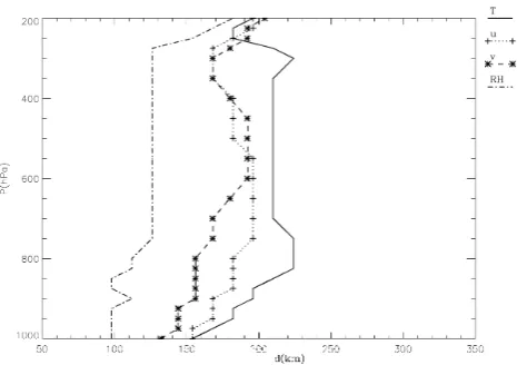
Fig. 1. Length scales (xaxis) of the different parameters of the
con-trol variable as a function of the pressure (yaxis).u is for zonal velocity,vis for meridional velocity,T is for temperature, and RH is for relative humidity.
atmospheric flow in the PBL generates features smaller than those of the free atmosphere.
The vertical transformUvis given by an empirical orthog-onal function (EOF) decomposition of the vertical compo-nent of the background error covariance matrix (Bz). To
de-termine Bz, the NMC method is firstly applied, by averaging
both in space (in longitude and latitude) and time, the dif-ference between 24 h and 12 h forecasts valid at the same time (see Appendix B for details). These simulations have the same grid configuration as the background run and have been interpolated onto the 3D-Var grid for the computation of the Bzmatrix. Hence the background error is computed on
the 3D-Var grid.
The variances of the model error are tuned after the ap-plication of the NMC method, as detailed in Appendix B. In fact, using the NMC method, the structure of the background error covariance is estimated as the average over many dif-ferences between two short-range model forecasts verifying at the same time, while the magnitude of the covariance is often appropriately scaled considering the problem at hand (see, for example, Kalnay, 2003; Sun et al., 2012; Barker et al., 2004).
The tuning factor chosen in this paper,t (var, p), depends on the variable and on the height (the 3D-Var system uses pressure as vertical coordinate) and is determined from the observational error (σo), which, in turn, depends on the vari-able and height.
The values ofσoare taken from the bibliography (Lazarus et al., 2002; Sashegyi et al., 1993). More in detail, the observational error is equal for the zonal and meridional wind components. It increases from 2.5 m s−1 at 1000 hPa to 4 m s−1 at 300 hPa. Then it decreases to 3.5 m s−1 at 200 hPa. Above 200 hPa the observational error for the veloc-ity components is held constant. For the relative humidveloc-ity, the
observational error is held constant (10 %) from 1000 hPa to 500 hPa, then it increases to 20 % at 200 hPa. Above 200 hPa the relative humidity is not assimilated. For the temperature, the observational error decreases from 1.8 K at 1000 hPa to 1.0 K at 800 hPa. Then it is held constant up to 500 hPa. The error increases from 1.0 K to 2.0 K between 500 and 300 hPa, and is held constant above this level.
In this paper, the tuning factort (var, p) is computed so that the variance of the model error is two times the vari-ance of the observational error for each variable and level. This choice is helpful in the context of this paper because the impact of a single observation on the analysis can be easily quantified.
It is worth noting that estimating the value of the forecast and observational errors is not an easy task because the NMC method provides only an approximation to the climatological component of the background error (Kalnay, 2003; Barker et al., 2004) and future studies will further focus on this prob-lem, also using the Lönnberg–Hollingsworth (1986) method. In this method the background and forecast errors are esti-mated from the differences between forecasts and observa-tions. However, the Lönnberg–Hollingsworth method has is-sues because the observational network often does not have enough density to allow a proper estimate of the error struc-ture.
Moreover, the choice of this paper of giving more credence to the observations than to the background could produce the problem of observations overfitting (Andersson et al., 1998), which worsen the forecast after a few hours.
As a consequence of the above issues, some assumptions must be made regarding estimating the observational and forecast errors, and sensitivity tests were done to support the choices made for this paper. In particular, numerical experi-ments were produced similar to that presented in this paper, but with the variance of the background error changed within a reasonable range (1–2) of the variance of the observational error. The results of these sensitivity tests show that, even if the performance of the data assimilation and forecasting sys-tem depends, in an absolute sense, on the choice of the ob-servational and forecast errors, the main conclusions of this paper remain unchanged.
By the application of the NMC method and of the tuning factors, the vertical component of the background error ma-trix Bz is obtained. The Bz is a block matrix, where each
block contains the vertical covariance between variables er-rors averaged in space and time:
Bz=
b(T , T ) b(T ,RH) b(T , u) b(T , v) b(RH, T ) b(RH,RH) b(RH, u) b(RH, v)
b(u, T ) b(u,RH) b(u, u) b(u, v) b(v, T ) b(v,RH) b(v, u) b(v, v)
(5)
S. Federico: Implementation of a 3D-Var system 3567
humidity, the zonal and meridional wind components, re-spectively.
The Bz matrix is symmetric and positive-defined and can
be decomposed in the eigenvalues and eigenvector matri-ces, i.e. Bz=VLVT, where V is the eigenvectors and L
the eigenvalues matrix. Using this decomposition, the ver-tical transformUvis written asUv=VL1/2.
The physical transformUpis applied to transform the con-trol variableν=(u0,v0,RH0,T0)to the model variable in-crementsx0=(Z0,u0,v0,RH0,T0), which differ only for the geopotential height increment.
The geopotential height increment is determined by the geostrophic equilibrium in pressure coordinates:
∇2
pZ
0=f ζ0
g , (6)
whereζ0 is the vertical component of the perturbed relative potential vorticity computed from the increments of the zonal (u0)and meridional (v0)wind components,g is the gravity (m s−2) andf is the Coriolis parameter (s−1).
The transformUp ensures the balance between the mass and wind increments. A future development of the analysis scheme will involve the implementation of a more sophisti-cated equation improving the mass–wind balance in regions where the geostrophic balance is a coarse approximation of the real flow, as the tropics or the PBL. For this purpose a statistical balance may also be employed. This approach is followed, for example, by Barker et al. (2004), who recover the pressurep, which plays the role of the geopotential height in their 3D-Var, by the equation
p=Cpb+pu, (7)
wherepbis the balanced pressure andpuis the unbalanced pressure. The unbalanced pressurepuis the control variable, whilepbis computed from a balance equation including cy-clostrophic terms. The correlation coefficient C, which is computed by the NMC method, provides a statistical filter-ing in regions where the balance equation is not appropriate. Finally, it is important to mention that it is assumed that the observational errors are uncorrelated with each other, so the matrix R in Eq. (2) is a diagonal matrix whose elements are all equal toσo2. The dimensions of the matrix R equal the number of measurements available at the analysis time.
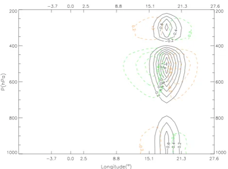
Figure 2 shows the combined effect of theUp,UvandUh transforms. It shows the longitude–height cross section at 57.5◦N latitude for the meridional velocity increments and
for the geopotential height increments determined by a sin-gle meridional wind component observation innovation of 2.5 m s−1, introduced over the Gotland Island ∼(57.5◦N, 18◦E) at 500 hPa. The final increment is spread vertically by theUv transform and horizontally byUh. TheUp trans-form determines the increments of the geopotential height. It is worth noting that a positive innovation of the meridional wind component at 500 hPa causes negative increments of
30 1
Fig. 1: Length-scales (x-axis) of the different parameters of the control variable as a function 2
of the pressure (y-axis). u is for zonal velocity, v is for meridional velocity, T is for 3
temperature, and RH is for relative humidity. 4
5
6
Fig. 2: The effect of the Uh , Uvand Up transforms (see text for details). Solid lines are 7
contours of meridional wind increments (v’, contours from 0. to 1.6 m/s with 0.2 interval); 8
dashed lines are the geopotential height increments Z’(contours from -0.6 to 0.6 m with 0.2 m 9
interval). 10
Fig. 2. The effect of theUh, Uv and Up transforms (see text for
details). Solid lines are contours of meridional wind increments (v0, contours from 0. to 1.6 m s−1with 0.2 interval); dashed lines are the geopotential height incrementsZ0(contours from−0.6 to 0.6 m with 0.2 m interval).
the same variable in the upper and lower troposphere. This is caused by the negative covariance between the vertical errors at 500 hPa and those in the upper and lower troposphere for the meridional wind component, as shown in Appendix B.
3 The experiment set-up
The background and the forecast are issued by the RAMS model (non-hydrostatic), version 6.0. Its physical settings are summarized in Table 1.
The analysis system and the RAMS model share the same horizontal coordinate system, which is a rotated polar stere-ographic projection, whose pole is near the centre of the do-main to minimize the projection distortion (Pielke, 2002). In the vertical direction, RAMS uses the sigma-zterrain follow-ing coordinate (Pielke, 2002), while the analysis uses pres-sure.
The possibility to run the analysis on the same horizon-tal coordinate system as RAMS, eventually with coarsened horizontal resolution to speed up the analysis, is an impor-tant feature because it simplifies the interpolation between the RAMS and analysis grids2.
3568 S. Federico: Implementation of a 3D-Var system
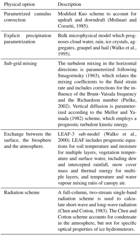
Table 1. RAMS model physical settings.
Physical option Description Parametrized cumulus
convection
Modified Kuo scheme to account for updraft and downdraft (Molinari and Corsetti, 1985).
Explicit precipitation parametrization
Bulk microphysical model which prog-noses cloud water, rain, ice crystals, ag-gregates, graupel and hail (Walko et al., 1995).
Sub-grid mixing The turbulent mixing in the horizontal directions is parameterized following Smagorinsky (1963), which relates the mixing coefficients to the fluid strain rate and includes corrections for the in-fluence of the Brunt–Vaisala frequency and the Richardson number (Pielke, 2002). Vertical diffusion is parameter-ized according to the Mellor and Ya-mada (1982) scheme, which employs a prognostic turbulent kinetic energy. Exchange between the
surface, the biosphere and the atmosphere.
LEAF-3 sub-model (Walko et al., 2000). LEAF includes prognostic equa-tions for soil temperature and moisture for multiple layers, vegetation temper-ature and surface water, including dew and intercepted rainfall, snow cover mass and thermal energy for multi-ple layers, and temperature and water vapour mixing ratio of canopy air. Radiation scheme A full-column, two-stream single-band
radiation scheme is used to calcu-late short-wave and long-wave radiation (Chen and Cotton, 1983). The Chen and Cotton scheme accounts for condensate in the atmosphere, but not for specific optical properties of ice hydrometeors.
25 hPa below 800 hPa. Above 300 hPa the vertical levels are unevenly spaced with a maximum distance of 25 hPa.
Observations used in this paper are vertical radiosondes (both land and ship) inside the analysis domain and wind measurement of the European wind profiler network. Both observing systems are shortly reviewed in Appendix A. Ra-diosondes reports contain vertical profiles of temperature, relative humidity, pressure, wind speed and direction, and are available at synoptic hours (00:00, 06:00, 12:00, 18:00 UTC) with few exceptions. The wind profilers measure the wind speed and direction in the vertical above the instrument and observations are available every one-hour.
Observations were downloaded from the MARS (Meteo-rological Archive and Retrieval System, see also http://www. ecmwf.int/publications/manuals/mars/) archive of ECMWF (European Centre for Medium Weather range Forecast) and the numerical experiment is performed for the month of July 2012.
Table 2. RAMS and analysis grid settings. NNXP, NNYP and
NNYZ are the number of grid points in the west–east, north–south, and vertical directions. Lx (km), Ly (km), Lz (m) are the domain extension in the west–east, north–south, and vertical directions. DX (km) and DY (km) are the horizontal grid resolutions in the west– east and north–south directions. CENTLON and CENTLAT are the geographical coordinates of the grid centres. The analysis grid uses pressure as vertical coordinate.
RAMS grid Analysis grid
NNXP 231 116
NNYP 231 116
NNZP 32 29
Lx 2520 km 2520 km Ly 2520 km 2520 km Lz 18800 m 1000–50 hPa
DX 10 km 20 km
DY 10 km 20 km
CENTLAT (◦) 50.0 50.0 CENTLON (◦) 8.0 8.0
A simple univariate quality control of the observations is adopted, which is based on the application of two checks in sequence. In the first step, the observations whose innova-tions are larger than four times the background error (σb)are discarded. This step avoids including observations affected by gross errors in the analysis. The second step is inspired by the cross-check of DiMego et al. (1985). In particular, each innovation is compared to the innovations located inside a circle whose radius is equal to three times the length scale of the recursive filters (Fig. 1). For each pair it is checked if the innovations are in reasonable agreement. Two inno-vations are in agreement if (a) they differ by less than one background error and their distance is less than one length scale of the recursive filter; and (b) the threshold of one back-ground error is increased up to 3.5 backback-ground errors for distances between innovations increasing from one to three length scales of the recursive filter. If the innovations are in agreement, a “hold” flag is assigned to the observation be-ing tested. The process is iterated for all observations. At the end of the process an observation is retained if (a) two or more cross-checks were done and at least two of them gave a “hold” result; (b) one cross-check was done and it gave a “hold” result; or (c) no cross-check could be done, i.e. iso-lated observations are retained if they pass the gross check.
S. Federico: Implementation of a 3D-Var system 3569
31 1
2
Figure 3: a) Background of the zonal wind component (m/s) at 850 hPa at 12 UTC on 01 July 3
2012; b) analysis increments (m/s) at the same time and level of a). The positions of the 4
radiosoundings (open squares) and of the wind profilers (filled circles) used in the analysis 5
are shown. The figure shows the horizontal domain used in this paper. 6
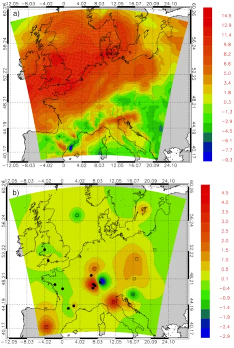
Fig. 3. (a) Background of the zonal wind component (m s−1) at
850 hPa at 12:00 UTC on 1 July 2012; (b) analysis increments (m s−1) at the same time and level of (a). The positions of the ra-diosondes (open squares) and of the wind profilers (filled circles) used in the analysis are shown. The figure shows the horizontal do-main used in this paper.
shows the effects of isolated observations on the analysed field, as over the North Sea.
To quantify the impact of the analysis both on the im-provement of the initial state and on the short-term forecast, the following strategy is adopted (Fig. 4). For each day of July 2012, one background run lasting 24 h is made starting at 00:00 UTC (hereafter also background run). Its initial and boundary conditions are taken every 6 h from the 00:00 UTC operational analysis/forecast cycle of ECMWF. These fields are available at 0.25◦horizontal resolution.
After 12 h of each run, an analysis is made. The 12:00 UTC was chosen because there are several radiosonde and wind profiler reports for this time. Table 3 shows the number of data used at the analysis times, accumulated over the whole period and over the whole domain (Fig. 3, Table 2), while Fig. 5a shows their vertical distribution, accumulated over the whole period. From Table 3 and Fig. 5a, it is noticeable
32 1
2
Figure 4: Synopsis of the simulations. BCKG is the background run, which lasts 24 h. ANL is 3
the analysis time: an analysis is performed at 12 UTC. FCST is the short-term forecast, which 4
lasts 3h. 5
6
7
8
Fig. 4. Synopsis of the simulations. BCKG is the background run,
which lasts 24 h. ANL is the analysis time: an analysis is performed at 12:00 UTC. FCST is the short-term forecast, which lasts 3 h.
that there are more data for the wind components because of the data from the European wind profiler network. Figure 5b shows the spatial distribution of the radiosondes and wind profilers at analysis time (12:00 UTC) for the whole period.
Starting from the analysis time, a short-term RAMS fore-cast, lasting 3 h, is made (hereafter also forecast run). For this run (a) the initial conditions are given by the analyses pro-duced at 12:00 UTC; and (b) the boundary conditions after 6 h are the same as the background run.
The root mean square error (RMSE) is computed between the background fields and observations, and between the forecast fields and observations for the whole period. The comparison of these statistics at the analysis time shows the performance of the data assimilation system; the same com-parison for times following the analysis time quantifies the impact of the analyses on the short-term forecast.
Statistics are presented for the zonal and meridional wind components only because few data are available for other variables after the analysis time. Indeed, temperature and relative humidity, which are measured by radiosondes, are available at synoptic times (00:00, 06:00, 12:00, 18:00 UTC) with few exceptions, while wind observations are available every one-hour by wind profilers measurements (Table 3). For example, Fig. 5c shows the vertical distribution of the data at 13:00 UTC for the whole period. Less than 5 obser-vations are available for temperature and relative humidity at all levels, while the number of data for the wind compo-nents varies from 309 (875 hPa) to 25 (130 hPa). From Fig. 5c it is apparent that statistics for temperature and relative hu-midity are reliable only at the analysis time and they will be briefly discussed in the next section. Finally, Fig. 5d shows the spatial distribution of the observational systems used at forecasting times (13:00, 14:00 and 15:00 UTC).
4 Results
3570 S. Federico: Implementation of a 3D-Var system
32 1
2
Figure 4: Synopsis of the simulations. BCKG is the background run, which lasts 24 h. ANL is 3
the analysis time: an analysis is performed at 12 UTC. FCST is the short-term forecast, which 4
lasts 3h. 5
6
7
8
33 1
2
3
4 33
1
2
3
4
34 1
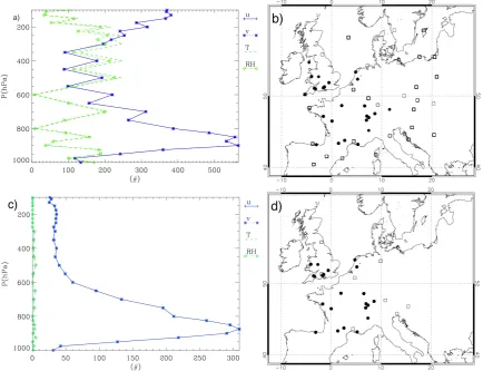
Figure 5: a) The number of data available at the analysis time (12 UTC) accumulated for the 2
whole period and over the whole domain. T is for temperature, RH is for relative humidity, u 3
and v are for the zonal and meridional wind components, respectively. The number of data for 4
the wind components (u, v) is the same for all levels; b) positions of the radiosoundings (open 5
squares) and radar wind profilers (filled circles) at 12 UTC considering the whole period. Not 6
all radiosoundings and radar wind profilers are reporting data at a specific analysis time; c) as 7
in a) for 13 UTC; d) positions of the radiosoundings (open squares) and radar wind profilers 8
(filled circles) at forecasting times (13, 14 and 15 UTC). Not all radiosoundings and radar 9
wind profilers are reporting data at a specific forecasting time. 10
11
12
Fig. 5. (a) The number of data available at the analysis time (12:00 UTC) accumulated for the whole period and over the whole domain.T
is for temperature, RH is for relative humidity, anduandvare for the zonal and meridional wind components, respectively. The number of data for the wind components (u, v)is the same for all levels; (b) positions of the radiosondes (open squares) and radar wind profilers (filled circles) at 12:00 UTC considering the whole period. Not all radiosondes and radar wind profilers are reporting data at a specific analysis time; (c) as in (a) for 13:00 UTC; (d) positions of the radiosondes (open squares) and radar wind profilers (filled circles) at forecasting times (13:00, 14:00 and 15:00 UTC). Not all radiosondes and radar wind profilers are reporting data at a specific forecasting time.
Table 3. Number of available data at analysis and forecasting times, accumulated over the whole period and over the whole domain.uis for
zonal velocity,vis for meridional velocity,T is for temperature, and RH is for relative humidity.
Radiosondes Wind profilers
Time Soundings number u, v T RH Soundings number u, v
12:00 UTC 458 5984 3993 3622 405 2684
13:00 UTC 5 57 / / 407 2763
14:00 UTC 8 73 / / 407 2744
15:00 UTC 9 90 / / 413 2802
considered and the statistics are computed for the whole do-main (Fig. 3).
It should also be emphasized that RMSE_f at the analy-sis time is computed after the analyses have been used to initialize the RAMS model. Hence, the difference between RMSE_b and RMSE_f accounts for the errors introduced by
the vertical interpolation between the RAMS and analysis grids.
S. Federico: Implementation of a 3D-Var system 3571
35 1
2
3
4
5
6
7
8
9
10
11
36 1
2
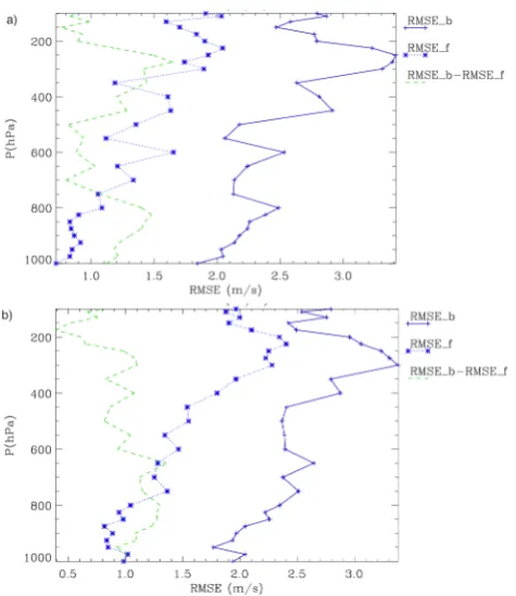
Figure 6: RMSE of the background field (RMSE_b), of the analyses (RMSE_f), and their 3
difference (RMSE_b-RMSE_f) for: a) zonal wind component; b) meridional wind 4
component. The RMSEs are computed for the whole period considering the grid-points 5
nearest to the observations. The RMSE_f statistics are computed after the RAMS model has 6
been initialized by the analyses. 7
8
9
Fig. 6. RMSE of the background field (RMSE_b), of the analyses
(RMSE_f), and their difference (RMSE_b−RMSE_f) for (a) zonal wind component and (b) meridional wind component. The RMSEs are computed for the whole period, considering the grid points near-est to the observations. The RMSE_f statistics are computed after the RAMS model has been initialized by the analyses.
(RMSE_f) decreases by more than 1.0 m s−1for most levels and RMSE_f is more than halved below 700 hPa.
Similar considerations apply for the meridional wind com-ponent (Fig. 6b), whose RMSE_f is∼1.0 m s−1lower than RMSE_b for several levels.
The analyses for both wind components show a decrease of the performance above 300 hPa, as shown by the decrease of the difference between RMSE_b and RMSE_f above this level.
For the other parameters (not shown) similar results are obtained, with a significant reduction of the error at the anal-ysis time (30–60 % of the background error). The improve-ment is comparatively larger at the lower levels.
Even if it is not simple to quantify the performance of the data assimilation scheme because it varies with the parameter and with height, a discussion is provided to clarify the results of Fig. 6.
First it should be noticed that the analyses effectively re-duce the error. The analysis RMSE is lowered by 30–60 % of the control forecast value for most levels and for all parame-ters; below 700 hPa, the RMSE reduction is often larger than 50 % of the background value.
The error reduction of 30–60 % of the control forecast value is in reasonable agreement with the setting of the data assimilation system. In particular, considering that the model error variance σb2 is twice the observational error variance σo2at all levels, and for the ideal case of one measurement available at a grid point of the analysis grid, the analysis at this point is closer to the observation than to the back-ground, and the error is more than halved. In particular, for this simple ideal case, it can be shown that the analysis er-ror (RMSE_f) isσo2/(σo2+σb2)of the control forecast error (RMSE_b; Kalnay, 2003), with an error reduction of 67 %.
The limit of this simple ideal case is not attained in the practical application of the analysis system mainly because the observations innovations, i. e. the differences between the background and observations, interact with each other both in the horizontal plane and vertically. This is shown, for exam-ple, by the analysis increments of Fig. 3b in central Europe.
It is interesting to consider the impact of the analysis on the short-term forecast.
Figure 7 shows the difference between RMSE_b and RMSE_f for the wind components. A positive difference means that the short-term forecast has a lower error than the control forecast and the wind forecast is effectively improved by using the analyses as initial conditions.
After the one-hour forecast, the improvement of the per-formance for the zonal velocity is apparent. In particular, the difference of the RMSE_b and RMSE_f is positive for all levels but 975 and 150 hPa, and it is larger than 0.5 m s−1for several levels. A useful statistic to represent the impact of the analysis on the short-term forecast is the vertically averaged value of the difference between RMSE_b and RMSE_f. This value is 1.15 m s−1for the analysis time and 0.43 m s−1for the one-hour forecast. From these values it follows that using the analyses effectively reduces the error (37 % of the value at the analysis time) after one-hour forecast.
After the two-hours forecast the improvement reduces. The vertical average of the difference between RMSE_b and RMSE_f is 0.20 m s−1, showing that the improvement is a sizeable fraction, i.e. larger than 10 %, of the initial value, and that the analysis is still effective at improving the short-term forecast.
For the three-hours forecast the impact of the analysis on the short-term forecast is negligible in practice. There are few levels for which the difference between RMSE_b and RMSE_f is negative, and its vertical average is 0.04 m s−1.
3572 S. Federico: Implementation of a 3D-Var system
36 1
2
Figure 6: RMSE of the background field (RMSE_b), of the analyses (RMSE_f), and their 3
difference (RMSE_b-RMSE_f) for: a) zonal wind component; b) meridional wind 4
component. The RMSEs are computed for the whole period considering the grid-points 5
nearest to the observations. The RMSE_f statistics are computed after the RAMS model has 6
been initialized by the analyses. 7
8
9
37 1
2
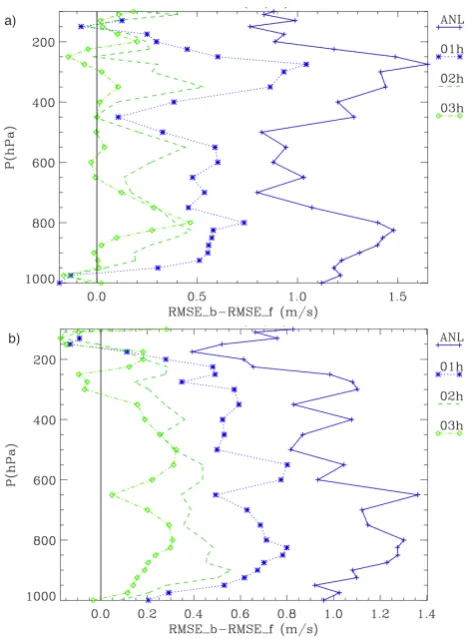
Figure 7: Differences between RMSE_b and RMSE_f for the analysis time (ANL), one- 3
(01h), two- (02h), and three-hours (03h) forecast for the: a) zonal wind component; b) 4
meridional wind component. The RMSEs are computed for the whole period considering the 5
grid-points nearest to the observations. The analysis time is shown to better understand the 6
behaviour of the performance with time. 7
Fig. 7. Differences between RMSE_b and RMSE_f for the analysis
time (ANL), one-(01 h), two-(02 h), and three-hours (03 h) forecast for the (a) zonal wind component and (b) meridional wind com-ponent. The RMSEs are computed for the whole period, consider-ing the grid points nearest to the observations. The analysis time is shown to better understand the behaviour of the performance with time.
short-term forecast above 200 hPa, caused by the compara-tively poorer performance of the analysis for upper levels.
Even though the improvement is reduced after the two-hour forecast, the difference between RMSE_b and RMSE_f is larger than 0.3 m s−1for several levels. The vertical aver-age of this difference is 0.27 m s−1, which is still a sizeable fraction (≈28 %) of its initial value.
After the three-hours forecast the improvement is smaller but still apparent for several levels in Fig. 7b. The vertical average of the difference between RMSE_b and RMSE_f is 0.11 m s−1.
It can be concluded that, for the setting of this paper, us-ing the analyses has a positive impact on the one-hour and two-hours forecasts for both wind components, with smaller positive impacts on the three-hours forecast.
This result is encouraging because the number of data used in the analysis is small. Moreover, it is in agreement with the numerical experiment settings. Indeed, consider-ing the wind components, which have the largest number of
measurements, the number of data used by the analysis is, on average, less than 15 for most levels (Fig. 5a). The analysis increments are centred at the observational point and have a radius of influence that depends on the height, but which is of the order of 100 km (Fig. 1). The analysis increments are advected downwind of the measurement point after a few hours, in agreement with the results of this section. It is ex-pected that, using a larger number of data, the positive impact of the analysis on the short–term forecast would last longer.
5 Conclusions
This paper presents the current status of development of a 3D-Var data assimilation system, tailored for the RAMS model, which is computationally fast and can be used in small meteorological centres.
The cost function is written in the incremental form. For the practical minimization of the cost function a variable transformation is used, which is composed of three trans-forms applied in sequence: the horizontal transformUh, the vertical transformUv, and then the physical transformUp.
The horizontal transform Uh is applied through recur-sive filters, which are computationally fast, while the ver-tical transform Uv is obtained through the eigenvalues– eigenvectors decomposition of the vertical component of the background error covariance matrix. The physical transform Upgives the geopotential height increments by applying the geostrophic balance to the wind increments. This ensures the balance between the increments of mass and wind fields.
The length scale of the recursive filters and the vertical component of the background error covariance matrix are es-timated by the NMC method.
A practical example is shown for the analysis/short-term wind forecast (0–3 h). Analyses are produced once a day at 12:00 UTC for the month of July 2012 with a horizontal reso-lution of 20 km and twenty-nine vertical levels. Observations are tropospheric profiles of wind, temperature and relative humidity from radiosondes, and tropospheric wind profiles from the European wind profiler network.
Analyses are effective at reducing the initial model error. The improvement is between 30 % and 60 % of the control forecast error for all parameters for most levels. It was shown that this improvement is in agreement with the data assimi-lation settings; nevertheless there is a decrease of the perfor-mance with increasing height partially caused by the errors introduced by the vertical interpolation between the RAMS and analysis grids.
The impact of the analyses on the short-term forecast is evaluated for the wind components only because there are few measurements at asynoptic times for other variables.
S. Federico: Implementation of a 3D-Var system 3573
Table A1. Characteristics of the radar wind profilers.
Frequency Antenna Power Range Resolution
(MHZ) size (m2) peak (kW) (km) (m) Name and description
50 10 000 250 2–20 150–1000 VHF wind profiler. Wind profilers used for sampling the troposphere and lower stratosphere.
400 120 40 0.2–14 250 UHF wind profiler. Wind profilers used for sampling the troposphere.
1000 5 0.5 0.1–5 60–100 Boundary layer wind profiler. Used to sample the lower troposphere.
for the two-hours forecast and for both wind components. The positive impact of the analysis after the three-hours fore-cast is reduced (4 % and 11 % of its value at the analysis time for the zonal and meridional wind components, respectively) but still evident for several levels.
It is concluded that, considering the amount of data used in the data assimilation, the results are encouraging and are in agreement with the set-up of the numerical experiment.
Work is in progress on several aspects of the data assim-ilation system. In particular, future development will con-sider (a) the inclusion of measurements coming from differ-ent sources; (b) a more sophisticated balance for theUp trans-form; and (c) an improved quality control of the observations. Nevertheless, the analysis system and the numerical experi-ment presented in this work should be of interest for the at-mospheric profiling community because it can be applied to OSE and OSSE experiments aiming to investigate the impact of the tropospheric profilers on the short-term wind forecast.
Appendix A
Observing systems
In this paper measurements from two observing systems are used: radiosondes and wind profilers. These instruments are shortly reviewed in this Appendix.
A1 Radiosondes
The radiosonde is a balloon-borne device measuring, in situ, the vertical profile of meteorological variables and transmits the data to a ground-based receiving station.
Vertical profiles of temperature, humidity, and pressure are given as the balloon ascends from the land or ocean surface to heights up to about 30 km. The profile of these meteorologi-cal variables is meteorologi-called an upper-air sounding that is known as a radiosonde observation or RAOB.
The radiosonde is carried aloft by a balloon, which is made of natural rubber (latex) or synthetic rubber (neoprene). Operational radiosonde systems typically use balloons that weight from 0.3 to 1.2 kg, filled to ensure an ascent rate of
300 m min−1. The meteorological measurements are made at intervals that vary from 1 to 6 s, depending on the radiosonde type.
Sensors used for pressure, humidity and temperature ob-servations are often of the capacitance type. Changes in pres-sure, temperature and/or humidity result in changes in the ca-pacitance of each sensor, which is converted to a frequency signal. Frequencies are converted to physical measurements by factory calibration measurements. Wind speed and direc-tion are determined by observing the drift of the balloon and high quality tracking information is necessary for ob-taining high quality wind measurements. Nowadays Global Positioning System (GPS) is of widespread usage because of its high accuracy and global coverage. A GPS receiver in-side the radiosonde measures directly the drift velocity of the balloon and hence the wind.
Countries launching operational radiosondes are members of the World Meteorological Organization’s World Weather Watch program. They launch radiosondes at 00:00 and 12:00 UTC (actually the launches occur 45 min before these observing times) and are contemporary worldwide to provide a synoptic description of the atmosphere. Countries of the World Weather Watch program freely share their sounding data with each other. After an operational upper-air sounding is completed, a standard data message (TEMP) is prepared and made available to all nations using the Global Telecom-munications System.
There are two main applications of radiosonde observa-tions: to analyse and describe current weather patterns, and to provide inputs to short- and medium-range weather fore-casting models. More details about radiosondes are provided by the World Meteorological Organization (WMO, 1996). A2 Wind profilers
3574 S. Federico: Implementation of a 3D-Var system
22 500 hPa causes negative increments in the lower and upper troposphere, as shown by the 1
negative vertical error covariance between these levels. This behaviour of the vertical error 2
covariance is clearly shown in Figure 2. 3
Finally, Figure B.2 shows the covariance between the meridional wind component at 900, 500 4
and 250 hPa, and the zonal wind component. There is a decrease of the absolute value of the 5
covariance compared to Figure B.1, as expected, and there is a rather complex interaction 6
between the two wind components as a function of the level. 7
8
Figure B.1: Vertical error covariance of the meridional wind component at 900 (diamonds), 500 (squares) and 9
200 (triangles) hPa. 10
11
200 300 400 500 600 700 800 900 1000
-‐20 -‐10 0 10 20 30 40
P(hPa)
cov(v,v); (m/s)^2
900 hPa 500 hPa 250 hPa
Fig. B1. Vertical error covariance of the meridional wind
compo-nent at 900 (diamonds), 500 (squares) and 200 (triangles) hPa.
amplified and discriminated in range by sampling it with de-lays of fixed intervals, which are built in the data processing system. In this way, the radar receives scattered energy from discrete altitudes, referred to as range gates.
In the troposphere and the stratosphere the backscattered energy is produced by small-scale fluctuations of the refrac-tive index, which are in turn produced by small-scale fluctu-ations in atmospheric density. These small-scale fluctufluctu-ations are produced by the turbulence and move with the bulk mo-tion of the medium in which they are embedded. The radar is most sensitive to the scattering by turbulent eddies whose spatial scale is half of the length scale of the electromagnetic radiation emitted by the radar (Table A1).
The Doppler frequency shift of the backscattered energy is determined and it is used to calculate the velocity of the air toward or away from the radar, along the direction of the emitted beam as a function of the height.
A typical configuration of the radar wind profiler is that of an antenna, which is both the transmitter and the receiver, emitting electromagnetic pulses in five directions: one is the vertical and the other four, tilted off the vertical, are orthog-onal to one another. The vertical beam is used to retrieve the vertical velocity, while the combination of all the beams is used to determine the horizontal wind components.
Finally, Table A1 shows the main characteristics of the radar wind profilers, including those of the European wind profiler network, used for wind profiling in the tropo-sphere/low stratosphere. More details about wind profilers can be found in Clifford et al. (1994).
Appendix B
The computation of the Bzmatrix
This Appendix shows how the vertical component of the background error covariance matrix (Bz)is derived and how
23 1
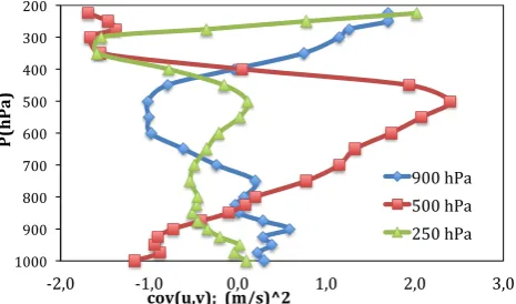
Figure B.2: Vertical error covariance between the meridional wind component at 900 (diamonds), 500 (squares) 2
and 200 (triangles) hPa and the zonal wind component. 3
4
5
Acknowledgements 6
Most of the elaborations of this work were performed on the ECMWF supercomputing 7
environment, in the framework of the special project SPITFEDE. I am grateful to the 8
“Aereonautica Militare Italiana” and to the ECMWF for the data and for their support in using 9
the MARS archive. I am grateful to Anna Trevisan for the helpful discussion and comments 10
on this paper. 11
12
References 13
Anderson, J.: An ensemble adjustment Kalman filter for data assimilation. Mon. Wea. Rev., 14
129, 2884–2903, 2001. 15
Andersson, E., Haseler, J., Undén, P., Courtier, P., Kelly, G., Vasiljevic, D., Brankovic, C., 16
Gaffard, C., Hollingsworth, A., Jakob, C., Janssen, P., Klinker, E., Lanzinger, A., Miller, M., 17
200
300
400
500
600
700
800
900
1000
-‐2,0 -‐1,0 0,0 1,0 2,0 3,0
P(hPa)
cov(u,v); (m/s)^2
900 hPa 500 hPa 250 hPa
Fig. B2. Vertical error covariance between the meridional wind
component at 900 (diamonds), 500 (squares) and 200 (triangles) hPa and the zonal wind component.
the tuning factors are applied. The methodology to compute Bzis detailed in the following points:
1. The difference between two short-term forecasts verifying at the same time is firstly computed x0(i, j, k, t )=x
T1(i, j, k, t )−xT2(i, j, k, t ), where
T1 = 12 h and T2 = 24 h, and i, j, k, t show the de-pendence of x0 on the three spatial dimensions and
time. In this paper the whole month of July 2012 was considered and the differences x0(i, j, k, t )were computed between two short-term forecasts verifying at 00:00 UTC on each day;
2. For each vertical level, the averagex(k, t )is computed to define anomalies:
v0(i, j, k, t )=x0(i, j, k, t )−x(k, t ) (B1) 3. The domain averaged vertical background error co-variance matrix B0(k, k0, t )is computed for each day:
B0(k, k0, t )= X
i=1,I;j=1,J
v0(i, j, k, t )v0(i, j, k0, t ) I J
(B2) 4. The matrices B0(k, k0, t ) are averaged in time to get the space and time averaged vertical component of the background error covariance matrix B0z:
B0z=B0z(k, k0)= X
t=1,T
B0(k, k0, t )
T (B3)
The elements of the covariance matrix B0zare tuned after this step, obtaining the vertical component of the background error covariance matrix Bz. The tuning coefficients are
S. Federico: Implementation of a 3D-Var system 3575
chosen for each variable and level so that the variance of the model error is two times the variance of the observational error.
More in detail, the matrix B0zmay be written as
B0z=
b0(T , T ) b0(T ,RH) b0(T , u) b0(T , v) b0(RH, T ) b0(RH,RH) b0(RH, u) b0(RH, v)
b0(u, T ) b0(u,RH) b0(u, u) b0(u, v) b0(v, T ) b0(v,RH) b0(v, u) b0(v, v)
(B4)
where,b0(var 1, var 2) is a square-matrix whose dimensions are equal to the number of levels of the analysis grid (29, Table 2), containing the vertical error covariance between the variables var 1 and var 2 computed from Eqs. (B1)–(B3);T, RH,uandvare the temperature, relative humidity, the zonal and meridional wind components, respectively.
The tuning factort (var, p)is computed so that
t (var, p)B0z(var,var, p, p)=2σo2(var, p), (B5) where B0z(var,var, p, p)are the diagonal terms of the B0z ma-trix (Eq. B4). Once the values oft (var, p)have been deter-mined, the square diagonal matrix D is formed containing the square root of the tuning factors ordered according to the ma-trix B0
z(Eq. B4). The vertical component of the background
error covariance matrix Bzis then computed as follows:
Bz=DB0zD. (B6)
The Bz matrix is symmetric and positive-defined and can
be decomposed in the eigenvalues and eigenvectors matri-ces, i.e. Bz=VLVT, whereV is the eigenvectors and L the
eigenvalues matrix. Using this decomposition, the vertical transformUvis written asUv=VL1/2.
Figure B1 shows the vertical covariance profiles from the Bzmatrix, i.e. after the application of the tuning factors, of
the meridional wind component for three levels, namely 900, 500, and 250 hPa.
The vertical error covariance shows a broader peak at 500 hPa compared to that in the upper and lower troposphere. Moreover, a positive increment of the meridional wind com-ponent at 500 hPa causes negative increments in the lower and upper troposphere, as shown by the negative vertical er-ror covariance between these levels. This behaviour of the vertical error covariance is clearly shown in Fig. 2.
Finally, Fig. B2 shows the covariance between the merid-ional wind component at 900, 500 and 250 hPa, and the zonal wind component. There is a decrease of the absolute value of the covariance compared to Fig. B1, as expected, and there is a rather complex interaction between the two wind compo-nents as a function of the level.
Acknowledgements. Most of the elaborations of this work were performed on the ECMWF supercomputing environment, within the framework of the special project SPITFEDE. I am grateful to the Aereonautica Militare Italiana and to the ECMWF for the data
and for their support in using the MARS archive. I am also grateful to Anna Trevisan for the helpful discussion and comments on this paper.
Edited by: D. Cimini
References
Anderson, J.: An ensemble adjustment Kalman filter for data assim-ilation, Mon. Weather Rev., 129, 2884–2903, 2001.
Andersson, E., Haseler, J., Undén, P., Courtier, P., Kelly, G., Vasil-jevic, D., Brankovic, C., Gaffard, C., Hollingsworth, A., Jakob, C., Janssen, P., Klinker, E., Lanzinger, A., Miller, M., Rabier, F., Simmons, A., Strauss, B., Viterbo, P., Cardinali, C., and Thépaut, J. N.: The ECMWF implementation of three-dimensional varia-tional assimilation (3D-Var). III: Experimental results, Q. J. Roy. Meteorol. Soc., 124, 1831–1860, 1998.
Barker, D. M., Huang, W., Guo, Y.-R., and Bourgeois, A.: Athree-dimensional variational (3DVAR) data assimilation system for use with MM5. NCAR Tech. Note. NCAR/TN-453 1 STR, avail-able from UCAR Communications, P.O. Box 3000,Boulder, CO 80307, 68 pp., 2003.
Barker, D. M., Huang, W., Guo, Y.-R., and Xiao, Q. N.: A Three-Dimensional Variational Data Assimilation System For MM5: Implementation And Initial Results, Mon. Weather Rev., 132, 897–914, 2004.
Chen, C. and Cotton, W. R.: A One-Dimensional Simulation of the Stratocumulus-Capped Mixed Layer, Bound.-Lay. Meteorol., 25, 289–321, 1983.
Clifford, S., Kaimal, J. C., Lataitis, R. J., and Strauch, R. G.: Ground-based remote profiling in atmospheric studies: an overview, P. IEEE, 82, 313–355, 1994.
Cotton, W. R., Pielke Sr., R. A., Walko, R. L., Liston, G. E., Tremback, C. J., Jiang, H., McAnelly, R. L., Harrington, J. Y., Nicholls, M. E., Carrio, G. G., and McFadden, J. P.: RAMS 2001: Current satus and future directions, Meteorol. Atmos., Phys., 82, 5–29, 2003.
Courtier, P., Thépaut, J. N., and Hollingsworth, A.: A strategy for operational implementation of 4D-Var, using an incremental ap-proach, Q. J. Roy. Meteorol. Soc., 120, 1367–1387, 1994. DiMego, G. J., Phoebus, P. A., and McDonell, J. E: Data
process-ing and quality control for optimum interpolation analyses at the National Meteorological Center, Washington, DC, US Dept of Commerce, National Oceanic and Atmospheric Administration, National Weather Service, Office Note 306, 1985.
Federico, S.: Preliminary Results of a Data Assimilation System, Atmospheric and Climate Sciences, 3, 61–72, 2013.
Huang, X. Y., Xiao, Q., Barker, D. M., Zhang, X., Michalakes, J., Huang, W., Henderson, T., Bray, J., Chen, Y., Ma, Z., Dudhia, J., Guo, Y., Zhang, X., Won, D. J., Lin, H. C., and Kuo, Y. H.: Four-Dimensional Variational Data Assimilation for WRF: Formula-tion and Preliminary Results, Mon. Weather Rev., 137, 299–314, doi:10.1175/2008MWR2577.1, 2009.
Kalnay, E.: Atmospheric Modeling, Data Assimilation and Pre-dictability, Cambridge University Press, 2003.
3576 S. Federico: Implementation of a 3D-Var system
Lazarus, S. M., Ciliberti, C. M., Horel, J. D., and Brewster, K. A.: Near-Real-Time Applications of a Mesoscale Analysis System to Complex Terrain, Weather Forecast., 17, 149–160, 2002. Lönnberg, P. and Hollingsworth, A.: The statistical structure of
short-range forecast errors as determined from radiosonde data. Part II: The covariance of height and wind errors, Tellus, 38A, 137–161, 1986.
Lorenc, A. C.: Analysis methods for numerical weather prediction, Q. J. Roy. Meteorol. Soc., 112, 1177–1194, 1986.
Mellor, G. and Yamada, T.: Development of a Turbulence Closure Model for Geophysical Fluid Problems, Rev. Geophys. Space Phys., 20, 851–875, 1982.
Molinari, J. and Corsetti, T.: Incorporation of cloud-scale and mesoscale down-drafts into a cumulus parametrization: results of one and three-dimensional integrations, Mon. Weather Rev., 113, 485–501, 1985.
Moninger, W. R., Benjamin, S. G., Jamison, B. D., Schlatter, T. W., Smith, T. L., and Szoke, E. D.: Evaluation of Regional Aircraft Observations Using TAMDAR, Weather Forecast., 25, 627–645, 2010.
Otkin, J. A., Hartung, D. C., Turner, D. D., Petersen, R. A., Feltz, W. F., and Janzon, E.: Assimilation of Surface-Based Boundary Layer Profiler Observations during a Cool-Season Weather Event Using an Observing System Simulation Experiment. Part I: Anal-ysis Impact, Mon. Weather Rev., 139, 2327–2346, 2011. Parrish, D. F. and Derber, J. C.: The National Meteorological
Center’s Spectral Statistical Interpolation analysis system, Mon. Weather Rev., 120, 1747–1763, 1992.
Pielke, R. A: Mesoscale Meteorological Modeling, Academic Press, San Diego, 2002.
Polkinghorne, R. and Vukicevic, T: Data assimilation of cloud-affected radiances in a cloud resolving model, Mon. Weather Rev., 139, 755–773, 2011.
Polkinghorne, R., Vukicevic, T., and Evans, K. F.: Validation of Cloud-Resolving Model Background Data for Cloud Data As-similation, Mon. Weather Rev., 138, 781–795, 2010.
Purser, R. J., Wu, W.-S., Parrish, D. F., and Roberts, N. M.: Nu-merical aspects of the application of recursive filters to vari-ational statistical analysis. Part I: Spatially homogeneous and isotropic Gaussian covariances, Mon. Weather Rev., 131, 1524– 1535, 2003.
Rabier, F., Järvinnen, H., Klinker, E., Mahfouf, J.-F., and Sim-mons, A.: The ECMWF operational implementation of four-dimensional variational assimilation. I: Experimental results with simplified physics, Q. J. Roy. Meteorol. Soc., 126, 1143–1170, 2000.
Sashegyi, D. K., Harms, D. E., Madala, R. V., and Raman, S.: Appli-cation of the Bratseth Scheme for the Analysis Of GALE, Data Using a Mesoscale Model, Mon. Weather. Rev., 121, 207–220, 1993.
Schenkman, A. D., Xue, M., Shapiro, A., Brewster, K., and Gao, J.: The Analysis and Prediction of the 8–9 May 2007 Oklahoma Tornadic Mesoscale Convective System by Assimilating WSR-88D and CASA Radar Data Using 3DVAR, Mon. Weather Rev., 139, 224–246, 2011.
Smagorinsky, J.: General circulation experiments with the primitive equations. Part I, The basic experiment, Mon. Weather. Rev., 91, 99–164, 1963.
Sun, J. and Crook, N. A.: Dynamical and microphysical retrieval from Doppler radar observations using a cloud model and its ad-joint. Part I: Model development and simulated data experiments, J. Atmos. Sci., 54, 1642–1661, 1997.
Sun, J. and Wang, H.: WRF-ARW Variational Storm-scale Data As-similation: Current Capabilities and Future Developments, Adv. Meteorol., 13, 815910, doi:10.1155/2013/815910, 2013. Sun, J., Trier, S. B., Xiao, Q., Weisman, M. L., Wang, H., Ying, Z.,
Xu, M., and Zhang, Y.: Sensitivity of 0–12-h Warm-Season Pre-cipitation Forecasts over the Central United States to Model Ini-tialization, Weather Forecast., 27, 832–855, doi:10.1175/WAF-D-11-00075.1, 2012.
Walko, R. L., Cotton, W. R., Meyers, M. P., and Harrington, J. Y.: New RAMS cloud microphysics parameterization part I: the single-moment scheme, Atmos. Res., 38, 29–62, 1995.
Walko, R. L., Band, L. E., Baron, J., Kittel, T. G., Lammers, R., Lee, T. J., Ojima, D., Pielke Sr., R. A., Taylor, C., Tague, C., Trem-back, C. J., and Vidale, P. L.: Coupled Atmosphere-Biosphere-Hydrology Models for environmental prediction, J. Appl. Mete-orol., 39, 931–944, 2000.
Wang, H., Sun, J., Zhang, X., Huang, X., and Auligne, T.: Radar data assimilation withWRF4D-Var. Part I: system development and preliminary testing, Mon. Weather Rev., 139, 2224–2244, doi:10.1175/MWR-D-12-00168.1, 2013.
World Meteorological Organization: Guide to Meteorological In-struments and Methods of Observation, 6th Edn., Publication No. 8. Geneva, WMO, 1996.
Zhang, F., Meng., Z., and Askoy, A.: Tests of an Ensemble Kalman Filter for Mesoscale and Regional-Scale Data Assimilation. Part I: Perfect Model Experiments, Mon. Weather Rev., 134, 722– 736, 2005.
Zou, X., Kuo, Y.-H., and Guo, Y.-R.: Assimilation of atmospheric radio refractivity using a nonhydrostatic mesoscale model, Mon. Weather Rev., 123, 2229–2249, 1995.