https://doi.org/10.5194/amt-10-2163-2017 © Author(s) 2017. This work is distributed under the Creative Commons Attribution 3.0 License.
AirCore-HR: a high-resolution column sampling to enhance the
vertical description of CH
4
and CO
2
Olivier Membrive1,2, Cyril Crevoisier1, Colm Sweeney3,4, François Danis1, Albert Hertzog1, Andreas Engel5, Harald Bönisch5, and Laurence Picon2
1Laboratoire de Météorologie Dynamique, IPSL, CNRS, École Polytechnique, Université Paris-Saclay, 91128, Palaiseau, France
2Laboratoire de Météorologie Dynamique, IPSL, CNRS, UPMC Université Paris 06, Sorbonne Universités, 75252, Paris, France
3Cooperative Institute for Research in Environmental Sciences, University of Colorado, Boulder, USA
4National Oceanic and Atmospheric Administration, Earth System Research Laboratory, NOAA/ESRL, Boulder, Colorado, USA
5Institute for Atmospheric and Environmental Sciences, University of Frankfurt, Frankfurt, Germany Correspondence to:Olivier Membrive ([email protected])
Received: 15 July 2016 – Discussion started: 26 September 2016
Revised: 8 February 2017 – Accepted: 7 April 2017 – Published: 12 June 2017
Abstract.An original and innovative sampling system called AirCore was presented by NOAA in 2010 (Karion et al., 2010). It consists of a long (>100 m) and narrow (<1 cm) stainless steel tube that can retain a profile of atmospheric air. The captured air sample has then to be analyzed with a gas analyzer for trace mole fraction. In this study, we introduce a new AirCore aiming to improve resolution along the vertical with the objectives to (i) better capture the vertical distribu-tion of CO2 and CH4, (ii) provide a tool to compare Air-Cores and validate the estimated vertical resolution achieved by AirCores. This (high-resolution) AirCore-HR consists of a 300 m tube, combining 200 m of 0.125 in. (3.175 mm) tube and a 100 m of 0.25 in. (6.35 mm) tube. This new configura-tion allows us to achieve a vertical resoluconfigura-tion of 300 m up to 15 km and better than 500 m up to 22 km (if analysis of the retained sample is performed within 3 h). The AirCore-HR was flown for the first time during the annual StratoScience campaign from CNES in August 2014 from Timmins (On-tario, Canada). High-resolution vertical profiles of CO2and CH4up to 25 km were successfully retrieved. These profiles revealed well-defined transport structures in the troposphere (also seen in CAMS-ECMWF high-resolution forecasts of CO2 and CH4 profiles) and captured the decrease of CO2 and CH4in the stratosphere. The multi-instrument gondola also carried two other low-resolution AirCore-GUF that
1 Introduction
Understanding the global atmospheric budget of the two ma-jor greenhouse gases (GHG) emitted by human activities, carbon dioxide (CO2) and methane (CH4), is essential for predicting their future concentration levels. To that end, sev-eral efforts have been dedicated to improving the monitoring capabilities of these gases. Under coordination by the World Meteorological Organization (WMO), a global atmospheric CO2and CH4monitoring network of surface-based stations has been established (GCOS, 2011) to provide continuous in-formation on their atmospheric concentrations. Although es-sential to infer surface fluxes, these surface measurements are sparse and lack information pertaining to the vertical struc-ture of the atmospheric CO2 and CH4. In order to improve spatial coverage, several satellite-based missions have been developed to monitor greenhouse gases from space. Obser-vations in the shortwave infrared (SWIR) enable the retrieval total atmospheric columns, during daytime and mostly over land. SWIR missions include the Scanning Imaging Absorp-tion Spectrometer for Atmospheric Chartography (SCIA-MACHY) spanning 2003–2012 (Frankenberg et al., 2011; Wecht et al., 2014), the Greenhouse Gases Observing Satel-lite (GOSAT) since 2009 (Hamazaki et al., 2007; Butz et al., 2011) and more recently the Orbiting Carbon Observatory (OCO-2) for CO2only (Crisp et al., 2004; Hammerling et al., 2012). Observations of terrestrial radiation in the thermal in-frared (TIR) provide information mostly on mid-tropospheric columns, by day and night, over land and sea. Missions in-clude the Atmospheric Infrared Sounder (AIRS) since 2002 (Crevoisier et al., 2003; Xiong et al., 2010), the Tropospheric Emission Spectrometer (TES) from 2004 to 2011 (Worden et al., 2012) and the Infrared Atmospheric Sounding Interfer-ometer (IASI) since 2007 (Crevoisier et al., 2009a, b, 2013; Xiong et al., 2013). Vertical profiles of CO2 and CH4 are also available from limb measurements such as from the At-mospheric Chemistry Experiment (ACE-FTS; Foucher et al., 2011). These satellite-based vertical profiles mainly cover the upper troposphere and low stratosphere (UTLS) with a low vertical resolution.
One of the main challenges for any satellite-based mea-surements is data evaluation and the comparability to WMO standards. To that end the Total Column Observing Network (TCCON; Wunch et al., 2010) has been established. It con-sists of a network of upward-looking Fourier transform spec-trometers (FTS) and has been widely used to evaluate re-trievals of total columns from SWIR space missions (e.g., Houweling et al., 2014). TCCON provides column-averaged retrievals that do not have any vertical resolution and also require independent evaluation of the data.
Precise and regular vertical profile measurements from the surface to above the tropopause are currently missing to eval-uate total or partial columns of GHG retrieved either from the ground or from space and to tie them to the calibrated mea-surements of the WMO.
Several aircraft missions contribute vertical information with regular measurements along commercial airlines such as the CONTRAIL project (Machida et al., 2008) and the CARIBIC project (Schuck et al., 2009). Other, less regular aircraft campaigns are also dedicated to study GHG at a lo-cal slo-cale (Zhang et al., 2014; Chen et al., 2010; Karion et al., 2013; Crevoisier et al., 2006, 2010; Sweeney et al., 2015) or from pole to pole such as the HIPPO project (Wofsy, 2011). Such vertical profiles are usually limited to 12 km.
To overcome this limitation, several instruments to mea-sure CO2 and CH4 profiles have been developed for de-ployment on high-altitude balloons. Commonly used tech-niques include FTS measurements such as the Michelson Interferometer for Passive Atmospheric Sounding (MIPAS; Oelhaf et al., 1991), cryogenic samplers (e.g., Schmidt and Khedim, 1991; Engel et al., 2008) to capture air in flasks at different altitudes along the balloon flight to be analyzed at a later stage, and laser-diode spectrometers such as the Spectromètre Infra Rouge pour l’Étude de l’Atmosphère par Diode Laser Embarquées (SPIRALE; Moreau et al., 2005) or Pico-SDLA instruments (Durry et al., 2004; Ghysels et al., 2011; Joly et al., 2007). All these instruments must be flown on heavy balloon-borne platforms. They can thus not be flown on a regular basis.
In this context, an original and innovative atmospheric sampling system called AirCore has been developed at the National Oceanic and Atmospheric Administration Earth System Research Laboratory (NOAA/ESRL; Karion et al., 2010) from an idea originally developed and patented by Pieter Tans (Tans, 2009). It consists of a long and thin stain-less steel tube shaped in the form of a coil which can sample the surrounding atmosphere and preserve a profile. This new system allows balloon measurements of GHG vertical pro-files from the surface up to approximately 30 km. The ver-tical resolution is ultimately determined by the length and diameter of the tubes.
Since the development of the first AirCore (Karion et al., 2010), new and lighter AirCores have been developed at NOAA, Groningen University and Goethe University Frank-furt. These lighter AirCores capture a smaller volume of air, leading to a slight decrease in the achievable vertical resolu-tion. This paper focuses on the development of an AirCore that allows the retrieval of profiles of GHG with a higher resolution along the vertical, with the following objectives: (i) to better capture the vertical distribution of atmospheric CO2 and CH4 in the troposphere, UTLS and stratospheric regions; and (ii) to provide a tool to compare low-resolution AirCores and validate the theoretical resolution achievable by AirCores.
low-Tube empes Tube samples ambient air
Tube is closed to preserve the sample Tube is filled with
calibrated standard
Connous gas analyzer Calibrated gas
The sample is measured with a connuous analyser for trace gas mole fracon
Ceiling
≈ 30 km
Surface 1. Preparaon
2. Ascent 3. Descent
4. Closed
5. Analysis Mixing raos of gases
CO2, CH4, CO… depending on the analyzer
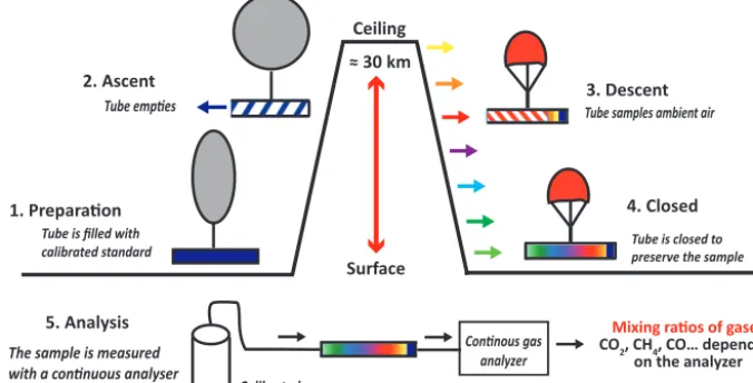
Figure 1.Schematic description of the five steps of the AirCore sampling method.
resolution profiles retrieved from two AirCores. Section 5 gives the conclusion.
2 AirCore-HR design, experimental setup and processing method
The general principle of an AirCore is illustrated in Fig. 1. First, in a preparation phase, the tube is filled with a cali-brated gas standard. It is placed under a balloon with one end of the tube open and the other end closed. During the ascent phase, as the air in the tube equilibrates with ambi-ent pressure, the initial fill gas evacuates. After reaching an upper limit, where only a small fraction of the initial fill gas remains in the tube, the AirCore starts a descent phase. Dur-ing this phase, as it maintains pressure equilibrium along the descent, the tube samples the ambient air. On the ground, the tube is closed, retaining the sampled profile to be analyzed with an analyzer for trace gas mole fraction.
2.1 Relation between AirCore design and vertical resolution
AirCores can be designed in a variety of configurations that determine the vertical resolution that can be achieved with the instrument. The resolution directly depends on the molec-ular diffusion and shear flow diffusivity, otherwise known as Taylor dispersion, inside the tube (Karion et al., 2010). The two major criteria in designing an AirCore are thus: (i) keep-ing the tubes diameter sufficiently thin to have a laminar flow at the sampling flow rates; and (ii) constraining the total weight to fit the specific flight requirements of their carrier (weather balloons, stratospheric balloons, planes, etc.) while allowing for sampling of a sufficient amount of air for the planned analysis.
2.1.1 Impact of diffusion and dispersion on the vertical resolution
As described in Karion et al. (2010), at the flow rates of gas entering the AirCore during flight (< 235 sccm; standard cubic centimeters per minute) and during analysis (30 to 120 sccm) the flow in the AirCore-HR is expected to be lam-inar. The transition between laminar and turbulent flow can be evaluated thanks to the dimensionless Reynolds number (Reynolds, 1883). Taking into account the useful parameters to describe the tubing of an AirCore Reynolds number can be expressed as follows:
Re=
Qdin
ν6in
, (1)
whereQis the flow rate expressed in m3s−1,dinthe inner diameter in meters,νcinematic viscosity (µρ) in m2s−1and
6in the surface of the inner disc of a section of the tube in m2.
Most of the AirCore configurations will have the fol-lowing characteristics: (i)ν, the cinematic viscosity of air (15.6×10⁻⁶ at 20◦C); (ii) the inner diameter of the tube (din=0.15 to 1 cm); (iii) 6in, the surface of an inner disc of a section of the tube 2π rint2 withrin=0.075 to 0.5 cm; and (iv) the flow rateQ≈0.7 cm3s−1during analysis (about 40 cm3min−1) and possibly up to 250 cm3min−1, which is equivalent to≈4 cm3s−1during the fast descent phases.
Such values yield a number of Reynolds between
1,36< Re<8,5. (2)
In all circumstances the flow in an AirCore is thus lami-nar sinceReis much inferior to 1750 (Peixinho and Mullin,
2006).
sam-pled pressure range varies continuously and repartition of the air along the AirCore thus evolves rapidly. It is only from the moment the total column is sampled and the final air reparti-tion reached that the described model is used to calculate the vertical resolution (i.e., from the moment the tube is sealed with the captured sample until the end of the analysis).
At first, during a given storage time before the payload is recovered only molecular diffusion will affect the sample. As described in Karion et al. (2010) the root mean square of the distance of molecular travel is given by
Xrms=
q
(2Dtrecovery), (3)
where D is the molecular diffusivity of the different molecules in the surrounding gas. In air, at 20◦C and 1000 hPa, D is 0.16 cm2s−1 for CO2, while for CH4 it is 0.23 cm2s−1 (Massman, 1998).trecovery is the waiting time before analysis.
Then, during analysis, both molecular diffusion and the Taylor dispersion affecting the sample have to be accounted for. During this phase the root mean square of the distance of molecular travel is given by
Xrms=
q
(2Defftanalysis), (4)
wheretanalysisis time needed for a parcel of the sampled air to reach the analyzer’s cell andDeffis the effective diffusion coefficient combining molecular diffusion and Taylor disper-sion given by
Deff=D+
a2V2
48D, (5)
where D is the molecular diffusivity of the different molecules in the surrounding gas,ais the tube’s inner radius, andV is the average velocity of the air inside the tube.
In addition to the effects of diffusion and dispersion, which are the main drivers of the resulting vertical resolution, the smearing effect of the cell of the analyzer during analysis has to be taken into account. The analyzer used in this study (Pi-carro cavity ring-down spectrometer (CRDS); G2310) pulls the sample at 110 sccm and measuring at 0.5 Hz makes one measurement every 3.7 scc (standard cubic centimeters). The analyzer cell has a standard volume of approximately 6 scc, since it is 35 cc in volume, but is maintained at 187 hPa (140 torr) and 45◦C. The volume of the cell needs to be flushed about three times for the air to be completely renewed (Stowasser et al., 2014).
To account for mixing in the volume of the cell of the an-alyzer, a Gaussian function characterized by the following standard deviationσcellis considered:
σcell= 1 2
Vcell
6in
=1
2ltube, (6)
whereVcell represents the volume of the cell,6inthe inner surface of a tube (π rin2) andltubethe AirCore length required to store the volume of the cell. A Gaussian function charac-terized by this standard deviation allows us to show that mix-ing impacts a distance in the AirCore where almost 3 times the volume required to fill the cell is stored.
As all mixing effects can be considered Gaussian, the total distance of diffusionXrmsto be considered is given by
Xrms=
r
2Dtrecovery+2Defftanalysis+( 1 2ltube)
2. (7)
Using Eq. (7) and knowing that air is distributed in the Air-Core as a linear function of total pressure column sampled, it is possible to evaluate the pressure range affected by mixing related to diffusion and dispersion. The factor of 2 in front of Xrmscomes from accounting for diffusion in both directions.
1P =Pmax
2Xrms
L , (8)
where1P represents the effective resolution and Pmax the pressure at the surface when the coil is closed.Lis the total length of the AirCore. In the case of two tubes or more,1P
can be calculated independently for each tube.
Using a standard atmosphere temperature profile it is then possible using the hydrostatic law to associate the atmo-spheric pressure with a given altitude. In order to best rep-resent the latitudes at which the AirCores are to be de-ployed, we used the average temperature profile of the rep-resentative TIGR (Thermodynamic Initial Guess Retrieval) dataset (Chedin et al., 1985, available at http://ara.abct.lmd. polytechnique.fr/index.php?page=tigr) for midlatitudes.
2.1.2 Aiming for a high-resolution AirCore
To appreciate the value of the AirCore-HR it is important to understand the factors that determine the resolution of an AirCore. The first factor is the sample cell of the analyzer that will limit the number of independent measurements over the sampled volume. The second factor is the diffusion distance (explained above) which, depending on the diameter of the tube and the lag between when air was sampled and when it is analyzed, will eventually limit the sampling resolution of the AirCore.
0 500 1000 1500 2000 2500 3000 1000 500 300 100 50 25 10
P
(
h
P
a
)
AirCore-HR
NOAA “original” AirCore AirCore-GUF
0 5 10 15 20 25 30
Expected vertical resolution (m)
A
lt
it
u
d
e
(
k
m
)
Figure 2.Comparison of the vertical resolution that can be expected
with different AirCores for CO2 measurements after 3 h storage
time before analysis: AirCore-HR (red), the original NOAA Air-Core (black) and AirAir-Core-GUF (blue).
tubes, one characterized by a small diameter at the end that remains closed and one characterized by a larger diameter at the end that remains open, allows us to keep a high resolution for the stratosphere (by storing the stratospheric part of the sampled profile in the tube with the smallest diameter) while still sampling a consequent volume of air thanks to the larger tube. To maximize the total volume of the AirCore-HR and limit the impact of the diffusion distance, the AirCore-HR was designed with tubes of two different diameters.
Figure 2 illustrates a comparison of the vertical resolu-tion of CO2measurements that can be expected for air sam-pled with different AirCores (for an analysis performed at 38.5 sccm, with a surface pressurePmaxof 1013.25 hPa and a given storage time of 3 h). The resolution achievable with the first AirCore designed by NOAA (Karion et al., 2010) is shown in black. After 3 h of waiting time before analysis, it is possible to achieve a vertical resolution of 250 m at 10 km and 1.2 km at 20 km.
In order to achieve a higher resolution along the whole atmospheric column, a design of a 300 m tube consisting of a 200 m of 0.125 in. (3.175 mm) tube and a 100 m of 0.25 in. (6.35 mm) tube linked together as one tube was selected for HR. The increase in overall volume of the AirCore-HR allows a significant increase in resolution throughout the whole sampled air column (Fig. 2) as well as an increase of the overall weight. The resolution of the AirCore-HR for CO2 is estimated to be better than 300 m up to 15 km and better than 500 m up to 22 km.
The resolution achievable by the lightweight AirCore-GUF designed and developed at Goethe University Frank-furt is also shown in Fig. 2. AirCore-GUF is a 100 m long combining three tubes: a 20 m long 8 mm tube, a 40 m long 4 mm tube and a 40 m long 2 mm tube. It has been designed
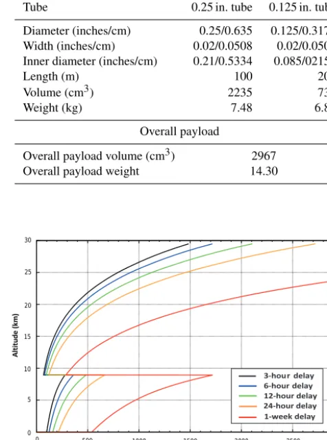
Table 1.Characteristics of the AirCore-HR.
Tube 0.25 in. tube 0.125 in. tube
Diameter (inches/cm) 0.25/0.635 0.125/0.3175
Width (inches/cm) 0.02/0.0508 0.02/0.0508
Inner diameter (inches/cm) 0.21/0.5334 0.085/02159
Length (m) 100 200
Volume (cm3) 2235 732
Weight (kg) 7.48 6.82
Overall payload
Overall payload volume (cm3) 2967
Overall payload weight 14.30
0 5 10 15 20 25 30
Altitude (km)
0 500 1000 1500 2000 2500 3000
Expected vertical resolution (m)
1-week delay 3-hou rdelay 6-hour delay 12-hour delay 24-hour delay
Figure 3.Impact of the time delay between landing and analysis on the expected vertical resolution of AirCore-HR, for a storage time of 3 h (black), 6 h (blue) and 12 h (green), 24 h (orange) and 1 week (red).
to be carried by meteorological balloons, resulting in com-promises between weight and achievable resolution. Thanks to a third tube with thinner diameter, it has a good resolution in the stratosphere (700 m at 20 km).
Flow restrictor (critical Ȍ Solenoid valve Regulator
Legend
AirCore-HR
Ǧway valve Calibration gas
cylinder 1
Protective box
Calibration gas cylinder 2
Bypass Picarro
gas analyzer Inlet
Pump
Outlet
Dryer
Outlet Inlet
Flow-meter Outlet
Analysis part Flying part
Figure 4.Overview of the AirCore-HR and analysis system.
2.2 AirCore-HR experimental setup
In order to obtain the vertical resolution shown in Fig. 2, the AirCore-HR comprises two tubes linked together as one, yielding an overall length of 300 m, a weight of 14.3 kg and an inner volume of 2.967 L. The detailed characteristics are given in Table 1. Both tubes have been treated by Restek, Inc., with Sulfinert® coating to reduce interactions of the sample with the walls.
The overall design is plotted in Fig. 4. Both sides of the coil are connected to three-way valves that allow ambient air to flow either through the AirCore-HR or through a bypass. This bypass consists in a 10 cm long, 0.0625 in. (1.5875 mm) diameter stainless steel tube that allows air to be pulled into the analyzer bypassing the AirCore-HR. During flight, in ad-dition to this setting, a dryer consisting of a short length (10 cm) of stainless steel tube filled with fresh magnesium perchlorate is positioned at the open end of the tube (at the entrance of ambient air on the solenoid valve) to ensure that no moisture enters the tubes during sampling. The additional volume to the system is very small and represents less than 0.005 % of the total volume (it is thus not considered in the calculation the vertical resolution; Sect. 2.1.1).
The AirCore-HR payload has been designed to fit into a polystyrene foam box. It is flown together with an electronic data package designed at LMD that collects meteorological data from a pressure sensor and three temperature probes and
also controls the opening and closing of a solenoid valve at the open end of the AirCore. Temperature probes are placed along the AirCore in contact with various segments of the tube and allow monitoring the mean temperature along the coil during the flight. The pressure sensor is an absolute pres-sure sensor that meapres-sures the ambient air prespres-sure during the flight.
2.2.1 Laboratory testing
Table 2. Values of the calibrated gas standards using NOAA’s WMO scale reference. The air of the two reference tanks used in this study was measured at LSCE with a Picarro G2401 calibrated with a scale of six tanks from NOAA/ESRL. The table shows the re-producibility of the measurements and standard deviation over three measurements made during a 15-day period.
Low-concentration standard
CO2360.85 ppm±0.008 ppm
CH41726.95 ppb±0.163 ppb
High-concentration standard
CO2401.31 ppm±0.004 ppm
CH41922.33 ppb±0.168 ppb
2.2.2 Atmospheric gas standards
For testing and analysis of the AirCores, two calibrated gas standards are used. The cylinders are connected to a multi-port valve, allowing selection of one of the gases.
The first standard is composed of high concentrations of CO2and CH4of, respectively, about 400 ppm and 1900 ppb and referred to as “high-concentration calibration standard”. The other standard is composed of lower concentrations of CO2and CH4of about 360 ppm and 1700 ppb, respectively, and referred to as “low-concentration standard”. The gas cylinders have been calibrated on WMO scales at Labora-toire de Sciences du Climat et de l’Environnement (LSCE; courtesy of Michel Ramonet and Marc Delmotte) and the ex-act calibrated values of the standard can be found in Table 2 where CO2 concentrations are given on the WMOX2007 scale and CH4concentrations are given on the NOAA-2004 scale.
2.2.3 The Picarro CRDS analyzer
All gas analyses of LMD AirCores were performed using one trace gas analyzer by Picarro, Inc., model G2310 (Crosson, 2008). The analyzer tightly controls the pressure and temper-ature in its measurement cell (187 hPa (140 torr) and 45◦C), to achieve the above precision (see Sect. 2.2.1). The sample flow rate was controlled by a critical orifice placed at the out-let, limiting the flow at 38.5 sccm during analysis.
2.3 Processing method
Upon recovery, the AirCore-HR is plugged into the prepared analysis system. It is first kept closed on both ends, allow-ing us to pull calibrated standards through the bypass into the analyzer. Once the values measured with the continuous analyzer are stabilized to the expected values for the cali-bration standard used as “push gas”, the analysis of the air captured in the coil can start. This phase is very important to make sure that, after plugging the AirCore-HR in the sys-tem, the mixing ratio read by the Picarro is not contaminated
CH
4
(ppb)
Analysis time(s)
Analysis time(s)
0 500 1000 1500 2000 2500 3000 3500 4000 4500 1000
1200 1400 1600 1800 2000
0 500 1000 1500 2000 2500 3000 3500 4000 4500 360
370 380 390 400
CO
2
(ppm)
(a)
(b)
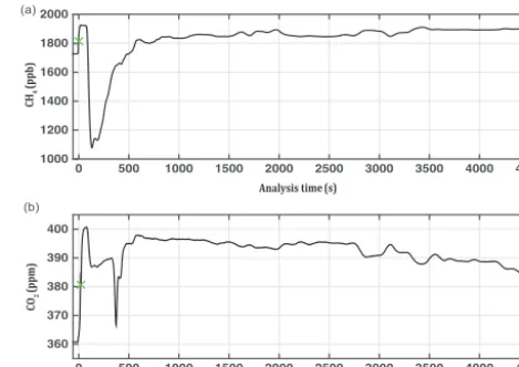
Figure 5.Picarro analysis of the AirCore-HR sample from the EdS-Stratéole flight on 29 August 2014.(a)CH4mixing ratios as a
func-tion of the analysis time in seconds;(b) CO2mixing ratios as a
function of the analysis time in seconds. The selected starting point of the sample is marked with a green cross and marks the 0 of the analysis time; the selected ending point of the AirCore-HR sample is marked with a red cross.
by water vapor that could have entered the analysis chain. The collected sample is then analyzed by opening both ends simultaneously; the air is pulled from one end into the con-tinuous analyzer and low-concentration calibration standard is pulled through the other end. The top of the profile with the remaining fill gas is pulled first into the analyzer.
The calibrated gas standards given in Table 2 allow replac-ing the values read by the Picarro onto the WMO scale. The high-concentration standard is used as fill gas to have a no-ticeable difference between fill gas and stratospheric air sam-ple at the top of the profile. The low-concentration calibration standard is chosen to be used as push gas to have a noticeable difference of the mixing ratios compared with the expected values of CO2and CH4at the surface.
Several steps are required to accurately place the Picarro measurements on a vertical scale in order to retrieve the verti-cal profiles. The dry mole fraction of CO2and CH4provided by the Picarro are used. These are automatically corrected by the instrument for a combined effect of dilution and line broadening caused by water vapor (Chen et al., 2010; Rella et al., 2013). Then, in a first processing step, the measured mixing ratios are corrected for a bias from the Picarro mea-surement to the WMO scales. The correction is calculated thanks to the measurement of the calibrated standards by the Picarro at the time of analysis.
concen-tration between the push gas and the remaining fill gas. This point corresponding to an estimated pressure of 0 hPa in the tube is marked with a green cross in Fig. 5. The bottom of the profile is defined at midpoint on the transition of concen-tration between push gas and sampled air. It is marked with a red cross in Fig. 5.
As a first approach, it is assumed that the air entering the tube equilibrates the sample with ambient pressure and adjusts very quickly with the mean coil temperature. As the characteristics of the AirCore (length, diameter) do not change, ambient pressure and mean coil temperature are the two main factors that regulate the number of moles in the AirCore. Using the ideal gas law (Eq. 9), it is possible to cal-culate the number of moles captured in the tube all along the trajectory.
P V =nRT ⇔n=P V
RT, (9)
where P is the ambient pressure, V the inner volume of the AirCore,nthe fraction of moles,Ris the universal gas constant in J K−1mol−1andT the ambient temperature in kelvin.
With measured time series of pressure (Pi) and
temper-ature (Ti; Fig. 7), it is possible to relate the number of air
moles in the tube (ni) to the atmospheric pressure at any
given time during the flight:
ni=
PiV
RTi
. (10)
This number is maximum when the AirCore reaches the Earth’s surface, i.e.,
nmax=PsV RTs
, (11)
wherePsandTscorrespond to the surface pressure and to the temperature of the AirCore when landing at the surface.
The critical orifice setting the flow during analysis at 38.5 sccm min−1 and the controlled settings of the Picarro analysis cell ensure that the same number of moles are ana-lyzed at every time step. In other words, during the sample analysis, the number of moles flown through the analyzer in-creases linearly with time. Hence, the number of moles at any time during the analysis is
ni=nmax
ti
1t, (12)
where1t is the total time duration of the analysis between the defined top and bottom of AirCore sample.
Using Eqs. (10) and (12), a specific pressure point can be associated with every Picarro measurement of the sample to retrieve the vertical profiles. Although the process is quite
simple, the selections of start and end point of the sampled profile in the Picarro data as well as in the temperature and pressure data are delicate steps that have a direct impact on the resulting profiles (see Sect. 4.2). Two additional effects need to be taken into account: the pressure loss along the tube (P. Tans, personal communiction, 2014) and the accounting of potential losses of air samples during the recovery process (see Sect. 3.2).
3 The StratoScience 2014 campaign
3.1 The EdS-Stratéole flight
AirCore-HR was flown for the first time during the Strato-Science campaign operated by the French space agency (CNES) in collaboration with the Canadian Space Agency (CSA) in Timmins (Ontario, Canada; 48.57 N,−81.36 E) in August 2014. It participated in the third flight of the cam-paign: the EdS (effet de serre– greenhouse effect) Stratéole flight.
The carrier consists of a gondola that could accommodate a total of eight instruments including the AirCore-HR. All these instruments (consisting of small packages of several kg) were brought together on the same structure with the aim of studying simultaneously several climate variables. In total, the gondola weighed 248 kg.
In addition to AirCore-HR, two AirCores-GUF from Goethe University Frankfurt were also flown during this flight.
3.2 Flight trajectory
To fulfill the requirements of the eight instruments, the EdS-Stratéole flight had a very specific flight trajectory. The take-off (release of the balloon) took place on 28 August 2014 at 20:33 local time in Timmins (00:33 UTC, 29 August 2014). After the ascent phase, the flight consisted of a monitored and controlled descent with two stops. Following a short stop at the ceiling at a barometric altitude of 14 hPa (29 km), an evacuation trap allowed us to let some gas out to engage in a descent phase down to a barometric altitude of 54 hPa (≈20 km); the balloon then stabilized in a slow descent phase for 6 h down to the barometric altitude of 78 hPa (≈18 km). The separation between the flight chain and the balloon did not take place at the ceiling as for weather balloon flights but at the end of this slow descent at a barometric altitude of 78 hPa. The two elements (flight chain and balloon envelope) were then separated and engaged separately in faster descent, both finally landing in a dry area 350 km southeast of Tim-mins at 07:28 local time (11:28 UTC, 29 August 2014).
AirCore-10 12 10
100
10000 2 4 6 8 14
10 12
10000 2 4 6 8 14
100
10 (a) AirCore-HR (b) AirCore-GUF
P (hP
a)
P (hP
a)
Time (hours) Time (hours)
Open (samples) Preparation phase
Open (empties) Closed at ceiling
Manually closed Preparation phase
Open (empties) Open (samples)
Closing system default Manually closed
Figure 6.Flight plan from the StratoScience 2014 EdS-Stratéole flight on 29 August 2014 with main operating states of(a)AirCore-HR and
(b)AirCore-GUF: the preparation phase, on the ground before flight (blue), ascent phase (green), descent phase (black) and closed (red).
HR was placed on the gondola and opened on one end just before takeoff. During the ascent phase (marked in green) the AirCore-HR emptied as it equilibrated with ambient pres-sure, thus evacuating fill gas. To preserve some part of the ini-tial fill gas in the coil the AirCore-HR was closed at 19 hPa (≈27 km) through a signal sent to the solenoid valve. The AirCore-HR remained closed at ceiling (marked in red) and was then reopened by sending another signal to the solenoid valve at 19 hPa during the descent phase. During all the de-scent phase (marked in black), the AirCore-HR remained open at one end. As the coil equilibrated with ambient sure, air was pulled into the tube. At landing, after the sure sensors on the electronic package detected no more pres-sure change, the solenoid valve closed in order to preserve the sample while waiting for recovery.
Joint efforts of CNES and CSA teams allowed access of the AirCores and analysis less than 3 h after landing. Unfor-tunately, at the end of the flight, the electronic circuit keeping the solenoid valve closed experienced a short power cut of about an hour, which resulted in sampled air evacuating from the AirCore. The AirCore-HR coil heated up after reaching the ground since it had been exposed to cold temperatures during the flight. During this period, the heating that occurred resulted in the loss of a fraction of the profile equivalent to the air sampled from 900 to 980 hPa. The loss of that fraction of the total sample had an impact on the retrieved vertical profiles (see Sect. 4.1).
The specific periods of interaction with ambient air of the AirCores-GUF are highlighted in Fig. 6b. The main differ-ence between AirCore-HR and AirCore-GUF was the lack of a closing device for the latter. The light AirCores from Goethe University Frankfurt thus remained open until recov-ery. Being less insulated than AirCore-HR and exposed to the same cold temperatures during flight, AirCores-GUF lost
0 2 4 6 8 10 12
101
102
103 -40
-30 -20 -10 0 10 20 30
Ambient pressure
Coil temperature
Time (hours)
P
(
h
P
a)
Te
m
p
er
at
u
re
(
°C
)
Figure 7. Recorded temperature from the three probes on the AirCore-HR and ambient pressure during the EdS-Stratéole flight on 29 August 2014. The three temperature probes (red, pink and purple lines) are presented in degrees Celsius as a function of time; the temperature axis is located on the right side. Ambient pressure (black line) is presented in hPa as a function of UTC time, with the vertical scale on the left side.
a fraction of the profile equivalent to the air sampled from about 780 to 980 hPa.
3.3 Measurement of additional data
800 1000 1200 1400 1600 1800 2000
1830 1840 1850 1860 1870 1880 1890 1900 1910 1920 200
300
400
500
600 700 800 900 1000
P (hP
a)
(b) CH4
CH4 (ppb)
103
102
101
Ambient T (K)
200 250 300
103
102
101
(c) Ambient temperature
P (hP
a)
P (hP
a)
(a) CO2
CO2 (ppm)
380 385 390 395 400
375
103
102
101
365 370
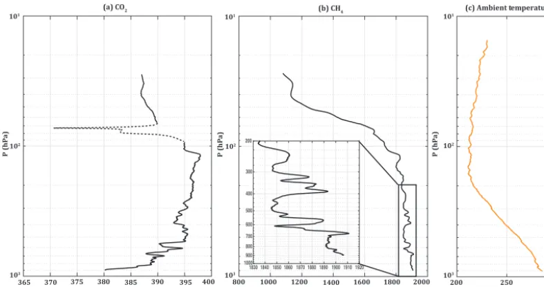
Figure 8.Vertical profiles retrieved from the air sampled with AirCore-HR on the EdS-Stratéole flight on 29 August 2014:(a)CO2(ppm),
(b)CH4(ppb) and(c)ambient temperature (K). The dotted line in the CO2profile corresponds to a part of the profile with unrealistic CO2
values due to flight trajectory (see text).
measured during the flight. The temperatures recorded by the three temperature probes during flight are plotted in red (full, dashed, points) and reported on the right y axis. Mean coil temperature is obtained by taking the mean of three temper-atures recorded by independent probes located at different positions along the AirCore-HR. The ambient pressure dur-ing the flight is plotted in black and reported on the left y
axis.
Comparison between AirCore-HR and other pressure measurements highlighted a small drift in AirCore-HR data pressure recordings. Therefore the pressure profile recorded with the electronics of AirCore-HR has been corrected to fit the high precision of the records of a Paroscientific, Inc., ab-solute pressure gauge that is characterized by an accuracy of 10 Pa and a precision of 0.1 Pa.
Additionally, GPS coordinates and altitudes from CNES were used to complete the dataset.
4 Results: the 0–25 km CO2and CH4
4.1 The profiles
Figure 8a and b show the CO2 and CH4 profiles measured during the StratoScience 2014 campaign. Each profile com-prises about 1800 points on the vertical. As explained in Sect. 3.2, profiles stop at 900 hPa due to the sample loss af-ter landing. Both CO2and CH4AirCore-HR vertical profiles reveal thin structures of the atmosphere and air-mass trans-port signatures. Figure 8c shows the ambient temperature recorded onboard during flight. From this ambient temper-ature profile the tropopause was estimated to be at 162.1 hPa
according to the definition of the WMO thermal tropopause (Reichler et al., 2003).
In Fig. 8a, a strong decrease of CO2can be observed in the first layers above ground. This is consistent with CO2 up-take by vegetation near the surface during the summer sea-son. CO2then reaches higher values in the free troposphere (∼393 ppm), with small variations (of 0.5–2 ppm) and two well-marked signatures at 700 and 600 hPa. CO2reaches its highest value of 396 ppm just above the tropopause. In the stratosphere, CO2values are expected to be lower since the exchange rate between upper troposphere and lower strato-sphere takes several years (Boering et al., 1981; Andrews et al., 2001; Engel et al., 2002). Above∼110 hPa, CO2 mix-ing ratios decrease slowly from 396 to 385 ppm at 30 hPa with one structure captured at the very top of the profile be-tween 30 and 40 hPa. This structure is correlated with a sim-ilar one at the same barometric altitude in the CH4profile in Fig. 8b.
per-800 1000 1200 1400 1600 1800 2000
1830 1840 1850 1860 1870 1880 1890 1900 1910 1920 200
300
400
500
600 700 800 900 1000
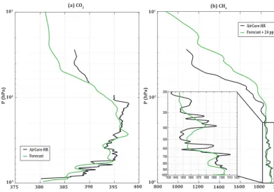
AirCore-HR Forecast
AirCore-HR Forecast + 24 ppb
P
(
h
P
a
)
P
(
h
P
a
)
(a) CO2 (b) CH4
CO2 (ppm) CH4 (ppb)
380 385 390 395 400
375
103 103
102 102
101 101
Figure 9.Comparison of AirCore-HR(a)CO2and(b)CH4vertical profiles (black) with co-located high-resolution forecast (green) from
CAMS-ECMWF at landing coordinates on 29 August 2014 at 12:00 UTC; 24 ppb were added to the CH4high-resolution forecast.
chlorate might have impacted CO2sampled by the AirCore-HR. Because the dryer is inert to CH4, no impact is seen on CH4 profile. Other explanations might be that the air sam-pled during this particular phase was polluted through inter-action with polystyrene, with the balloon envelope (pumping up some of the ambient air as they re-equilibrate with ambi-ent air during this long phase) or by chemical interaction with helium from the balloon (during some short reascent phases). The CH4vertical profile is presented in Fig. 8b. Mixing ratios of CH4have a small variability in the troposphere be-tween 1800 and 1880 ppb. The zoom on the tropospheric part (between 200 and 1000 hPa) reveals pronounced structures captured in the troposphere, particularly in the region from 200 to 700 hPa. These could be caused by transport or vari-ability in the emissions. The strong decrease of CH4in the stratosphere is particularly easy to see in Fig. 8b, with values of∼1800 ppb near the tropopause at 120 hPa to 1100 ppb at 30 hPa. Along the slopes, several structures can be identified around 80 hPa and between 30 and 40 hPa, revealing trans-port patterns in the stratosphere.
A comparison between Fig. 8a and b shows CO2 vari-ability is higher near the ground, whereas CH4 variability is higher in the mid-to-upper troposphere and in the strato-sphere. This is in agreement with the fact that CO2 may have negative and positive anomalies at the surface (associ-ated mainly with vegetation uptake and anthropogenic emis-sions), whereas CH4has mostly positive anomalies coming
from the surface and negative anomalies coming from the stratosphere.
A comparison was performed with CO2 and CH4 fore-casts from the Copernicus Atmosphere Monitoring Ser-vice (CAMS) using the European Centre for Medium-range Weather Forecasts (ECMWF) model (Agustí-Panareda et al., 2014; Massart et al., 2014). This comparison is presented in Fig. 9. The tracer transport in the forecast is constrained with meteorological observations by re-initializing the fore-cast every 24 h with operational ECMWF analyses, whereas the atmospheric CO2 and CH4 tracers are cycled from one 1-day forecast to the next, as in a free run. There-fore, the forecast is essentially a model simulation with state-of-the-art representation of tracer transport available in forecast mode (http://macc.copernicus-atmosphere.eu/d/ services/gac/nrt/rt_fields_ghg). The CAMS-ECMWF CO2 and CH4forecasts used here have a horizontal resolution of around 16 km×16 km and a vertical resolution of 137 lev-els from the surface to 0.01 hPa. These forecasts have been collocated in space and time with AirCore-HR landing co-ordinates. 24 ppb were added to the CAMS-ECMWF CH4 high-resolution forecast to emphasize the good agreement on structures rather than focusing on the bias, which may be at-tributed to incorrect surface fluxes or issues with air-mass exchanges along the vertical.
The forecast correctly reproduces the strong decrease in CO2 from 800 hPa to the surface, as well as the increase in con-centration from 800 to 600 hPa and a lower increase from 600 hPa. In the upper troposphere, from 300 hPa up to the tropopause at 150 hPa, the forecast displays different struc-tures than those measured by the AirCore-HR. In the lower stratosphere (from 150 to 90 hPa), the AirCore-HR and the CAMS-ECMWF forecasts both reveal a decrease in CO2 starting from just above the tropopause up to the top of the stratosphere.
Although fewer vertical structures are seen in the forecast, the CH4 mixing ratios and position of the broader vertical structures fit quite well with the measurements up to 200 hPa (Fig. 9b). For lower pressures, the decrease of CH4 mea-sured by AirCore-HR is much more pronounced than the one simulated by the forecast. This is a known problem in the CAMS-ECMWF model, which is currently being inves-tigated (A. Agusti-Panareda, S. Massart, personal communi-cation, 2016) and was also discussed in Verma et al. (2016).
4.2 Associated uncertainties
Monte Carlo simulations were performed to assess the uncer-tainty associated with the retrieved constituent profiles. The retrieval process of the vertical profiles was iterated a 1000 times by randomly changing the original datasets within the estimated uncertainty range of every identified uncertainty source. This allowed us to produce a set of 1000 slightly dif-ferent outcomes for the vertical profiles in terms of both mix-ing ratios and vertical position. A standard deviation of the mixing ratios at a given position was then calculated based on this dataset. In these simulations we took into account the following uncertainties:
i. The accuracy of the gas analyzer: Picarro measurement accuracy was defined as a Gaussian standard deviation of the mixing ratios based on the instrument specifica-tion (i.e., deviaspecifica-tions of 0.5 ppb for CH4 and 0.07 ppm for CO2; Crosson, 2008).
ii. The mean temperature profile: to account for the impact of temperature correction, the temperature profile was randomly chosen among the three profiles measured by the three probes. Indeed, the three temperature probes are placed at different positions along the tube (near the entrance, in the middle of the AirCore and near the closed end) and, depending on the distance to the in-let, they have recorded different temperatures along the AirCore. Choosing randomly between one of the three probes is thus the conservative way to account for the uncertainty related to the mean temperature of the Air-Core.
iii. The pressure profile: an uncertainty of 0.1 Pa corre-sponding to the accuracy of the Paroscientific, Inc., ab-solute pressure gauge was used.
P
(
h
P
a
)
CO2 (ppm)
(a) (b) (c)
CO2 (ppm) CO2 (ppm)
380 390 400
101
102
103
0 0.5 1
101
102
103
0 0.5 1
101
102
103
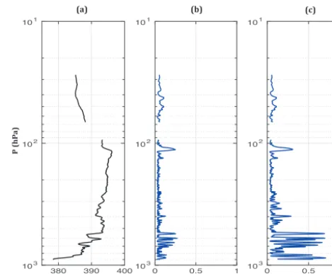
Figure 10. (a)AirCore-HR CO2vertical profile,(b)CO2
uncer-tainty without taking the potential loss of air into account (see Sect. 4.2, point v) and(c)overall CO2uncertainty.
iv. The selection of the sample: the choice of the exact mid-point of transition between either push gas and sample or remaining gas and sample (see Sect. 2.3) has an im-pact on the altitude of both ends of the profile. A ran-dom uncertainty of±1 Picarro measurement point was defined for both uncertainties.
v. The potential loss of air sample resulting from the tube remaining open after landing as occurred during this flight (see Sect. 3.2): an uncertainty of±10 hPa was as-sociated with the bottom pressure correction that was defined to take the air loss into account.
(a) (b) (c)
1000 1500 2000 101
102
103
0 5 10 101
102
103 0 5 10 101
102
103
P
(
h
P
a
)
CH
4 (ppb) CH4 (ppb) CH4 (ppb)
Figure 11. (a) AirCore-HR CH4vertical profile,(b) CH4
uncer-tainty without taking the potential loss of air into account (see Sect. 4.2, point v) and(c)overall CH4uncertainty.
Comparing Fig. 10b with Fig. 10c and Fig. 11b with Fig. 11c shows that, for both CO2and CH4, the uncertainty related to the bottom pressure correction has an important impact on the uncertainties estimated in the troposphere, al-though in the stratosphere the uncertainties remain relatively unaffected by this. Indeed the fraction of the overall uncer-tainties (Figs. 10c and 11c) that is related to the loss of air is above 80 % in the troposphere and drops to about 30% in the stratosphere. The dominating uncertainty source in the stratosphere is related to the selection of the sample. Mis-selecting the transition point between the gas in the AirCore sample and the calibrated standard by only one measurement has an important impact on the positioning of the strato-spheric part of the profiles. Indeed, the whole stratostrato-spheric air sampled by the AirCore accounts for about 8 % of the total sample (∼150 points out of ∼1800 total points) but corresponds to≈15 km of the 25 km profile. Hence, a differ-ence of a single measurement point in the positioning of the profile does matter.
Additionally, the impact of the variability in the measure-ments of the three temperature probes has been studied. It was found that temperature uncertainty has a very limited influence on the overall uncertainties, of the order of 6 %, despite differences of several degrees Celsius (Fig. 7). Al-though differences up to several degrees Celsius are observed between the measurement, the overall variation of the tem-perature is captured similarly by the three temtem-perature probes (Fig. 7). The increase of sampled moles in the AirCore at each pressure level as well as the total number of sampled moles in the AirCore are almost unchanged when consider-ing one or the other temperature sensor. This comes from the fact that, during the fast descent phase in the troposphere
when most of the sampled air is captured, the temperature remains very stable.
Overall, the average uncertainty on the CO2 profile (Fig. 10c) is 0.24 ppm throughout the column. The average uncertainty in the troposphere is 0.25 ppm with relatively higher uncertainties in the bottom of the profile where im-portant variations of CO2 are measured, indicating that the slightest positioning uncertainty translates into mixing ra-tio uncertainties. For the whole stratosphere above 120 hPa, where the CO2profile is more stable, the average uncertainty drops to 0.11 ppm.
The average uncertainty on the overall CH4 profile (Fig. 11c) is 2.78 ppb. In the stratosphere, above the tropopause at 120 hPa, CH4uncertainties are quite variable along the profile and can be as high as 10 ppb locally but on average are estimated to be 6.42 ppb. Such high values stem directly from high vertical gradients in mixing ratios: in that case, the assumed error on the vertical positioning of the pro-files translates into higher uncertainties. In the troposphere, the average uncertainty for the CH4 profile is below 2 ppb with sometimes values up to 5 ppb where the vertical profile shows transport structures of 30 ppb or more along the verti-cal in the troposphere.
4.3 Comparison between AirCores with different resolutions
4.3.1 Overall comparison
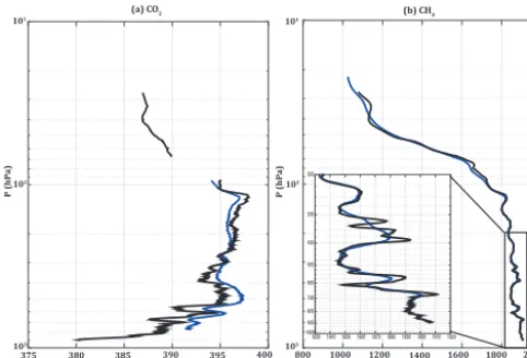
Benefiting from the accommodation of several AirCores on board the CNES gondola, the AirCore-HR profiles can be compared with those of the lighter AirCores-GUF (see Sect. 3). AirCore-GUF air samples were processed at LMD using the same methodology as for AirCore-HR (Sect. 2.3). The processing took into account the fact that AirCores-GUF remained open for 3 h before being manually closed at re-covery leading to the loss of the bottom of the profile be-tween 980 and 780 hPa (see Sect. 3.2). Both AirCore-GUF being identical, the comparison is presented with only one AirCore-GUF in order to focus on the comparison between AirCores with different resolutions. Figure 12a and b show the comparison of AirCore-HR and one AirCore-GUF CO2 and CH4profiles.
The particular descent profile of this flight had several im-pacts on the AirCore-GUF profiles:
i. As for AirCore-HR, unrealistic low values of CO2were sampled during the long plateau phase that happened between 70 and 90 hPa.
800 1000 1200 1400 1600 1800 2000
1830184018501860187018801890190019101920 200
300
400 500 600 700 800 900 1000
P
(
h
P
a
)
P
(
h
P
a
)
(a) CO2 (b) CH4
CO2 (ppm) CH4 (ppb)
380 385 390 395 400
375
103 103
102
102
101
101
Figure 12.Vertical profiles retrieved from the air sampled with the AirCore-HR and an AirCore-GUF on the EdS-Stratéole flight on 29
August 2014.(a)CO2(ppm);(b)CH4(ppb). The dotted line in the
CO2profiles corresponds to unrealistic CO2values sampled during
the long plateau phase (see Sect. 3.2).
whereas it was stored over the 100 m/0.25 in. (6.35 mm) tube for AirCore-HR. This led to a more intense diffu-sion in the AirCore-GUF sample.
Therefore, all the CO2 sampled above 100 hPa with AirCore-GUF was probably altered by the combination of unrealistic low values of CO2 acquired during the plateau phase and the diffusion effects. This part of the profile that should not be considered is shown in dotted line as with AirCore-HR CO2. Only AirCore-GUF CO2sampled in the troposphere below 100 hPa should be compared, where resid-ual effects from this phase are minimal. Concerning CH4, which was not impacted by the dryer during the plateau phase, only the difficulty of properly modeling the diffusion inside the tube remains. The full AirCore-GUF CH4profile is shown but the stratospheric part of the profile should thus be taken with caution.
The comparison between AirCore-HR (black) and AirCore-GUF (blue) highlights that both CO2 profiles (Fig. 12a) have a good agreement in terms of structures. In particular, the impact of vertical resolution is seen in Fig. 12a, with less structures captured by the lower-resolution AirCore. However, there is a variable but notice-able bias between the profiles (up to 3 ppm in some part of the profiles).
For CH4, Fig. 12b reveals that the agreement is excellent between AirCore-HR and AirCore-GUF. The zoom on the tropospheric part (between 200 and 1000 hPa) shows that the different AirCores capture the same structures and allow us to retrieve similar vertical profiles in terms of both struc-tures and mixing ratios albeit at a different resolution. In the stratosphere, both AirCores capture the position and incli-nation of the decreasing slope of methane. However, some stronger differences can be seen in terms of mixing ratios
between both profiles between 70 and 90 hPa or between 30 and 40 hPa. In these ranges, similar structures are captured by both AirCores but seem to be very strongly impacted by diffusion in the AirCore-GUF CH4 profile. This illustrates the impact of diffusion, which is stronger for AirCore-GUF than for AirCore-HR during the long plateau phase.
Overall, the comparison between both AirCores reveals that the high resolution captures more information on the ver-tical distribution along the atmospheric column.
4.3.2 Degradation of the resolution
To perform a fair comparison between the different AirCore profiles, the degradation of the resolution of AirCore-HR profiles to that of lower-resolution AirCore-GUF has to be performed. This exercise aims also to evaluate the theoreti-cal theoreti-calculation of the expected resolution (Sect. 2.1).
The vertical resolutions shown in Fig. 2 were calculated for a standard atmosphere and air sampled from 10 hPa to a ground pressure of 1013.25 hPa. In order to account for the sampling that occurred during flight and how the sampled air was distributed within the tubes, the vertical resolution of AirCores-GUF was recalculated with the specific parameters of the flight for both CO2and CH4.
Degradation of the AirCore-HR profiles is performed through the convolution with a Gaussian window with a stan-dard deviation of the lower vertical resolution at each given altitude:
g(x)= 1
σ √
2πexp(
−x
2
2σ2), (13)
whereσis the standard deviation (i.e., the vertical resolution) at a given vertical positionx.
It allows retrieving a degraded version of the profiles: degraded XCH4(x0)=
Z
CH4(x)g(x−x0)dx. (14)
The degraded version of the CO2profile is calculated simi-larly. To avoid the parts of the profiles that may have been affected by the strong diffusion during the long plateau phase in the flight profile, the comparison with degraded AirCore-HR profiles is only presented for pressures higher than 200 hPa.
The effect of the degradation of the AirCore-HR pro-file to the lower resolution of AirCore-GUF is presented in Figs. 13a and 14a. The differences between AirCore-GUF and the smoothed version of AirCore-HR (degraded to the vertical resolution of AirCore-GUF) are shown in Figs. 13b and 14b.
380 382 384 386 388 390 392 394 396 398 400 200
300
400
500
600
700
800
900
1000
P
(
h
P
a
)
(a)
CO2 (ppm)
AirCore-HR )
AirCore-HR degraded resolution AirCore-GUF
LMD
(b)
-1 -0.5 0 0.5 1 1.5 2 2.5 3
200
300
400
500
600
700
800
900
1000
P
(
h
P
a
)
CO2 (ppm)
Figure 13. (a)CO2vertical profiles from AirCore-HR in full resolution (black), from AirCore-HR in “degraded resolution” (pink) and from
AirCore-GUF (blue).(b)Residual of the difference AirCore-GUF−AirCore-HR in “degraded resolution”.
-3 -2 -1
200
300
400
500
600
700
800
900
1000
0 1 2 3
1830 1840 1850 1860 1870 1880 1890 1900 1910 1920 200
300
400
500
600
700
800
900
1000
P
(
h
P
a
)
(a)
CH4 (ppb) AirCore-HR )
AirCore-HR degraded resolution AirCore-GUF
LMD
(b)
CH4 (ppb)
P
(
h
P
a
)
Figure 14. (a)CH4vertical profiles from AirCore-HR in full resolution (black), from AirCore-HR in “degraded resolution” (pink) and from
AirCore-GUF (blue).(b)Residual of the difference AirCore-GUF−AirCore-HR in “degraded resolution”.
−1 ppm at 200 hPa up to 3 ppm at 780 hPa. The reasons of these observed differences are still debated. The main hy-potheses are that it could be related to some kind of “memory effect” of the tubing to the previously stored calibrated gas or the individual dryers from different AirCores may affect the CO2 samples slightly differently when capturing CO2. Overall, the problem highlights that there are some
remain-ing questions regardremain-ing CO2sampling and that some poten-tial interferences with CO2have to be studied more closely.
and +2.1 ppb (Fig. 14b), which is in agreement with the 2.8 ppb average uncertainty that can be associated with the AirCore-HR profile (see Sect. 4.2). In addition to allowing the comparison of AirCore-HR profiles with those of lower-resolution AirCores, the excellent agreement of both CH4 profiles validates the computation of theoretical vertical res-olution presented in Sect. 2.1.2.
5 Conclusions
In this paper, a new AirCore (AirCore-HR) allowing high-resolution measurements of CO2and CH4from the ground up to almost 30 km is presented. Thanks to the combination of two tubes, it allows retaining air samples with a vertical resolution better than 500 m up to 20 km when the analysis is performed within 6 h after landing of the instruments. As for any AirCore, the final resolution depends on the delay between landing and analysis.
The AirCore-HR was flown for the first time on a multi-instrument gondola, which allowed us to perform compar-isons of the vertical profiles retrieved with AirCore-HR and lower-resolution AirCore-GUF. The degradation of the pro-file given by AirCore-HR to the resolution of AirCore-GUF revealed an excellent agreement between both profiles for CH4, which fully validates the theory behind AirCores.
CO2 profiles retrieved from the AirCores on this flight have revealed unexpected structures between 60 and 90 hPa when the flight experienced a long plateau phase of about 7 h during descent, not seen on CH4. It is suspected that the magnesium perchlorate used as drying agent at the inlet of the AirCores inert to CH4may have played a role in the al-teration of CO2during this particular phase at low pressure. Moreover, the comparison of CO2 profiles has highlighted that the agreement is good in terms of structures but an im-portant and variable bias is seen between profiles. This bias is also suspected to come from potential interaction with the dryer and shows that CO2sampling aspects with AirCores as well as these potential impacts of the drying agent have to be further studied. Therefore, specific tests are planned during the future StratoScience 2017 campaign that will take place in March–April 2017 in Alice Springs, Australia. These tests will include comparing several independent AirCores flown on the same gondola with and without a dryer at inlet.
By designing a method that takes into account all the sources of uncertainties in the processing of the data, the overall uncertainty is estimated to be less than 3 ppb on the CH4profile and less then 0.3 ppm on the CO2profile. A par-ticular issue during the flight with the closing system has led to the loss of part of the sampled air. Therefore the highest pressure point sampled by the AirCore-HR had to be rected. An uncertainty of 10 hPa was associated with this cor-rection and it was estimated that this uncertainty is responsi-ble for∼80 % of the overall uncertainty on the profiles. In an ideal case where the system would close and retain the
com-plete sample, it would be possible to know more precisely the pressure at which air was sampled last and thus to improve the overall uncertainty to about 0.1 ppm for CO2and 2 ppb for CH4.
Comparison between AirCore data and forecasts from CAMS-ECMWF has yielded satisfying agreements between AirCore-HR profiles and simulated profiles. In particular, well-pronounced vertical transport signatures in the tropo-sphere in both CO2 and CH4 profiles are similar for both the forecasts and AirCore-HR profiles. In the stratosphere, the AirCore-HR CH4profile seems to indicate that the de-crease of stratospheric CH4in the forecasts is too slow, which may have an important impact when deriving total or partial columns of CH4from the analyses.
This comparison illustrates the potential of AirCores to evaluate atmospheric transport models, as well as GHG satel-lite retrievals from TIR and SWIR instruments. In particu-lar, light AirCores flown from weather balloons could be de-ployed at various locations to complete an effective system together with ground stations and regular aircraft campaigns. Such lightweight systems could also contribute to specific campaigns for calibration and validation of future space mis-sions. In order to fit these applications, the spatial and tempo-ral resolution requirements necessary to evaluate the models or satellite retrievals efficiently need to be assessed.
Along with the development of robust lightweight sys-tems, it is also important to continue development strate-gies of AirCores for large platforms carrying heavy payloads. Such platforms, flown during specific stratospheric balloon campaigns, allow unique multi-instrument measurements of the same or complementary atmospheric variables. The si-multaneous use of laser-diode spectrometers, cryosamplers and AirCores, which can only be performed during these spe-cific campaigns, is necessary to evaluate the retrievals per-formed with various AirCores and test improvements of the instruments.
Data availability. AirCore data presented in this paper are avail-able via the Ether database through the following link: http:// cds-espri.ipsl.upmc.fr/etherTypo/index.php?id=1792&L=1.
Competing interests. The authors declare that they have no conflict of interest.
ECMWF provided collocated CAMS-ECMWF data generated using Copernicus Atmosphere Monitoring Service Information (2016) and are to be thanked for their valuable input and scientific discussions. The development and deployment of AirCore at GUF was funded by the German Federal Ministry of Education and Research (BMBF) within the ROMIC program under project 01LG1221A.
Edited by: M. Hamilton
Reviewed by: two anonymous referees
References
Agustí-Panareda, A., Massart, S., Chevallier, F., Boussetta, S., Bal-samo, G., Beljaars, A., Ciais, P., Deutscher, N. M., Engelen, R., Jones, L., Kivi, R., Paris, J.-D., Peuch, V.-H., Sherlock, V., Vermeulen, A. T., Wennberg, P. O., and Wunch, D.:
Forecast-ing global atmospheric CO2, Atmos. Chem. Phys., 14, 11959–
11983, https://doi.org/10.5194/acp-14-11959-2014, 2014. Andrews, A. E., Boering, K. A., Daube, B. C., Wofsy, S. c.,
Loewen-stein, M., Jost, H., Podolske, J. R., Webster, C. R., Herman, R. L., Scott, D. C., Flesch, G. J., Moyer, E. J., Elkins, J. W., Dutton, G. S., Hurst, D. F., Moore, F. L., Ray, E. A., Romashkin, P. A., and Strahan, S. E.: Mean ages of stratospheric air derived from in situ observations of CO2, CH4, and N2O, J. Geophys. Res.-Biogeo., 106, 32295–32314, 2001.
Boering, K., Wofsy, S., Daube, B., Schneider, H., Loewenstein, M., Poldolske, J., and Conway, T.: Stratospheric mean ages and trans-port rates from obM servations of carbon dioxide and nitrous ox-ide, Science, 274, 1340–1343, 1981.
Butz, A., Guerlet, S., Hasekamp, O., Schepers, D., Galli, A., Aben, I., Frankenberg, C., Hartmann, J.-M., Tran, H., Kuze, A., Keppel-Aleks, G., Toon, G., Wunch, D., Wennberg, P., Deutscher, N., Griffith, D., Macatangay, R., Messerschmidt, J.,
Notholt, J., and Warneke, T.: Toward accurate CO2 and CH4
observations from GOSAT, Geophys. Res. Lett., 38, L14812, https://doi.org/10.1029/2011GL047888, 2011.
Chedin, A., Scott, N. A., Wahiche, C., and Moulinier, P.:
The Improved Initialization Inversion Method: A High
Resolution Physical Method for Temperature Retrievals
from Satellites of the TIROS-N Series, J. Clim. Appl.
Meteorol., 24, 128–143,
https://doi.org/10.1175/1520-0450(1985)024<0128:TIIIMA>2.0.CO;2, 1985.
Chen, H., Winderlich, J., Gerbig, C., Hoefer, A., Rella, C. W., Crosson, E. R., Van Pelt, A. D., Steinbach, J., Kolle, O., Beck, V., Daube, B. C., Gottlieb, E. W., Chow, V. Y., Santoni, G. W., and Wofsy, S. C.: High-accuracy continuous airborne
measure-ments of greenhouse gases (CO2and CH4) using the cavity
ring-down spectroscopy (CRDS) technique, Atmos. Meas. Tech., 3, 375–386, https://doi.org/10.5194/amt-3-375-2010, 2010. Crevoisier, C., Chedin, A., and Scott, N. A.: AIRS channel selection
for CO2and other trace-gas retrievals, Q. J. Roy. Meteorol. Soc.,
129, 2719–2740, 2003.
Crevoisier, C., Gloor, M., Gloaguen, E., Horowitz, L. W., Sarmiento, J. L., Sweeney, C., and Tans, P. P.: A direct carbon budgeting approach to infer carbon sources and sinks. Design and synthetic application to complement the NACP observation network, Tellus B, 58, 366–375, 2006.
Crevoisier, C., Chédin, A., Matsueda, H., Machida, T., Armante, R., and Scott, N. A.: First year of upper tropospheric integrated
content of CO2from IASI hyperspectral infrared observations,
Atmos. Chem. Phys., 9, 4797–4810, https://doi.org/10.5194/acp-9-4797-2009, 2009a.
Crevoisier, C., Nobileau, D., Fiore, A. M., Armante, R., Chédin, A., and Scott, N. A.: Tropospheric methane in the tropics – first year from IASI hyperspectral infrared observations, Atmos. Chem. Phys., 9, 6337–6350, https://doi.org/10.5194/acp-9-6337-2009, 2009b.
Crevoisier, C., Sweeney, C., Gloor, M., Sarmiento, J. L., and Tans, P. P.: Regional US carbon sinks from three-dimensional
atmo-spheric CO2 sampling, P. Natl. Acad. Sci. USA, 107, 18348–
18353, 2010.
Crevoisier, C., Nobileau, D., Armante, R., Crépeau, L., Machida, T., Sawa, Y., Matsueda, H., Schuck, T., Thonat, T., Pernin, J., Scott, N. A., and Chédin, A.: The 2007–2011 evolu-tion of tropical methane in the mid-troposphere as seen from space by MetOp-A/IASI, Atmos. Chem. Phys., 13, 4279–4289, https://doi.org/10.5194/acp-13-4279-2013, 2013.
Crisp, D., Atlas, R. M., Breon, F. M., Brown, L. R., Burrows, J. P., Ciais, P., Connor, B. J., Doney, S. C., Fung, I. Y., Jacob, D. J., Miller, C. E., O’Brien, D., Pawson, S., Randerson, J. T., Rayner, P., Salawitch, R. J., Sander, S. P., Sen, B., Stephens, G. L., Tans, P. P., Toon, G. C., Wennberg, P. O., Wofsy, S. c., Yung, Y. L., Kuang, Z., Chudasama, B., Sprague, G., Weiss, B., Pollock, R., Kenyon, D., and Schroll, S.: The Orbiting Carbon Observatory (OCO) mission, Adv. Space Res., 34, 700–709, 2004.
Crosson, E.: A cavity ring-down analyzer for measuring atmo-spheric levels of methane, carbon dioxide, and water vapor, Appl. Phys. B, 92, 403–408, https://doi.org/10.1007/s00340-008-3135-y, 2008.
Durry, G., Amarouche, N., Zeninari, V., Parvitte, B., Lebarbu, T., and Ovarlez, J.: In situ sensing of the middle atmosphere with balloonborne near-infrared laser diodes, Spectrochim. Acta A, 60, 3371–3379, 2004.
Engel, A., Strunk, M., Müller, M., Haase, H.-P., Poss, C., Levin, I., and Schmidt, U.: Temporal development of to-tal chlorine in the high-latitude stratosphere based on
ref-erence distributions of mean age derived from CO2 and
SF6, J. Geophys. Res.-Atmos., 107, ACH 1-1–ACH 1-11,
https://doi.org/10.1029/2001JD000584, 2002.
Engel, A., Möbius, T., Bönisch, H., Schmidt, U., Heinz, R., Levin, I., Atlas, E., Aoki, S., Nakazawa, T., Sugawara, S., Moore, F., Hurst, D., Elkins, J., Schauffler, S., Andrews, A., and Boering, K.: Age of stratospheric air unchanged within uncertainties over the past 30 years, Nat. Geosci., 2, 28–31, 2008.
Foucher, P. Y., Chédin, A., Armante, R., Boone, C., Crevoisier, C., and Bernath, P.: Carbon dioxide atmospheric vertical pro-files retrieved from space observation using ACE-FTS solar occultation instrument, Atmos. Chem. Phys., 11, 2455–2470, https://doi.org/10.5194/acp-11-2455-2011, 2011.