Nonlin. Processes Geophys., 20, 239–248, 2013 www.nonlin-processes-geophys.net/20/239/2013/ doi:10.5194/npg-20-239-2013
© Author(s) 2013. CC Attribution 3.0 License.
EGU Journal Logos (RGB)
Advances in
Geosciences
Open Access
Natural Hazards
and Earth System
Sciences
Open Access
Annales
Geophysicae
Open Access
Nonlinear Processes
in Geophysics
Open Access
Atmospheric
Chemistry
and Physics
Open Access
Atmospheric
Chemistry
and Physics
Open Access
Discussions
Atmospheric
Measurement
Techniques
Open Access
Atmospheric
Measurement
Techniques
Open Access
Discussions
Biogeosciences
Open Access Open Access
Biogeosciences
DiscussionsClimate
of the Past
Open Access Open Access
Climate
of the Past
Discussions
Earth System
Dynamics
Open Access Open Access
Earth System
Dynamics
Discussions
Geoscientific
Instrumentation
Methods and
Data Systems
Open Access
Geoscientific
Instrumentation
Methods and
Data Systems
Open Access
Discussions
Geoscientific
Model Development
Open Access Open Access
Geoscientific
Model Development
Discussions
Hydrology and
Earth System
Sciences
Open Access
Hydrology and
Earth System
Sciences
Open Access
Discussions
Ocean Science
Open Access Open Access
Ocean Science
Discussions
Solid Earth
Open Access Open Access
Solid Earth
Discussions
The Cryosphere
Open Access Open Access
The Cryosphere
Natural Hazards
and Earth System
Sciences
Open Access
Discussions
Estimation of the local response to a forcing in a high dimensional
system using the fluctuation-dissipation theorem
F. C. Cooper1, J. G. Esler2, and P. H. Haynes3
1Atmospheric, Oceanic and Planetary Physics, University of Oxford, Oxford, UK 2Department of Mathematics, University College, London, UK
3Department of Applied Mathematics and Theoretical Physics, University of Cambridge, Cambridge, UK Correspondence to: F. C. Cooper ([email protected])
Received: 1 August 2012 – Revised: 22 February 2013 – Accepted: 28 February 2013 – Published: 26 April 2013
Abstract. The fluctuation-dissipation theorem (FDT) has been proposed as a method of calculating the response of the earth’s atmosphere to a forcing. For this problem the high di-mensionality of the relevant data sets makes truncation nec-essary. Here we propose a method of truncation based upon the assumption that the response to a localised forcing is spa-tially localised, as an alternative to the standard method of choosing a number of the leading empirical orthogonal func-tions. For systems where this assumption holds, the response to any sufficiently small non-localised forcing may be esti-mated using a set of truncations that are chosen algorithmi-cally. We test our algorithm using 36 and 72 variable ver-sions of a stochastic Lorenz 95 system of ordinary differen-tial equations. We find that, for long integrations, the bias in the response estimated by the FDT is reduced from∼75 % of the true response to∼30 %.
1 Introduction
An important problem in atmospheric sciences is how the cli-mate responds to a forcing. For example how does the mean local temperature respond to an increase in carbon dioxide or a change in the incident solar radiation. Explicit simula-tion can estimate the effects of a particular forcing; however, simulation can be prohibitively expensive if the response to a large set of possible forcings is required. One method of reducing the cost of a local estimate is to truncate the cal-culation to a local simulation at a high resolution forced by boundary conditions given by a low resolution global simu-lation. For estimating the response to a forcing applied over a short time this regional approach seems effective, (see for
example the UK Met office numerical weather prediction model Davies et al., 2005); however, it remains to be seen if it can be extended to the long time climate response. The hy-pothesis explored in this paper is that a statistical approxima-tion based upon the fluctuaapproxima-tion-dissipaapproxima-tion theorem (FDT), using only data on the unforced system, will have some skill in predicting the response to a forcing. The form of the FDT that we consider predicts only the linear component of the response, i.e. the response of a (fully non-linear) system to a sufficiently small forcing, and much in the same way that simulation is expensive in computational effort, the FDT is expensive in data. Some sort of truncation is necessary to re-duce the quantity of data required. In this paper we describe a method of truncating a data set locally for the purposes of applying the FDT. This method, inspired by the technique of local simulation at high resolution, is a practical alternative to the globally distributed truncation to a particular number of empirical orthogonal functions (EOFs); see Joliffe (2002) chapter 6. The linear nature of the FDT then allows for the responses calculated with local truncation to many small lo-calised forcings to be added together to give the global re-sponse to a forcing that is not localised.
The expected responseδx(t )of a system to a forcing as a function of timetis denoted by
hδx(t )i = hxf(t )i − hx(t )i,
wherex(t )represents the state vector of the system without forcing applied,xf(t )represents the state vector of the
sys-tem with the forcing applied and the angled bracketsh. . .i
denote the ensemble average over a large number of inde-pendent realisations. Assuming that the system is sufficiently random and that its probability density function (PDF)ρ (x)
is differentiable, the linear component ofhδx(t )iis given by
hδx(t )i = − t Z
0 *
x(τ )
∇xρ (x(0)) ρ (x(0))
T+
δf(t−τ )dτ , (1)
whereδf(t )represents a forcing vector at timet and T de-notes the vector transpose; see for example Marconi et al. (2008) for a recent review. Throughout this paper we make the assumption that the mean ofx has been subtracted and thereforehx(t )i =0.
For practical evaluation of (1) knowledge ofρ (x)is re-quired. If it is assumed thatρ (x)is well approximated by a Gaussian, (1) reduces to the Gaussian FDT (sometimes called the quasi-Gaussian FDT)
hδx(t )i ≈ t Z
0
C(τ )C(0)−1δf(t−τ )dτ , (2)
where C(τ ) is the lag τ covariance matrix. Gritsun and Branstator (2007) amongst others have applied (2) to atmo-spheric general circulation model simulations with promis-ing results. The Gaussian FDT requires the inversion of a covariance matrix which can be difficult when considering a large state vectorx. In order to evaluate (2) Gritsun and Branstator reduced the size of their state vector by first se-lecting particular variables and truncating their system from 18 352 components to 1800 EOFs. Majda et al. (2010) sug-gests some strategies for truncation in EOF space, however, a general quantitative theory for such truncation, e.g. predict-ing any biases introduced, has not yet been developed.
In the context of global climate modelling aspects of the dynamical system, such as separation of timescales associ-ated with hydrostatic and geostrophic balance, can be ex-ploited to facilitate truncation. For example, Ring and Plumb (2008) use the solution of an “Eliassen problem” based on geostrophic balance to truncate an idealised general circula-tion model by expressing all variables in terms of the zonal wind. Their truncation is then used, for example, to convert a particular forcing of global temperature into an equivalent forcing of the zonal wind, that can then be used in a truncated version of (1).
One problem with (2) is that the assumption of Gaussianity where it is not appropriate may cause unacceptably large er-rors in a response prediction (Cooper and Haynes, 2013). An alternative approach, appropriate for short time responses, is to use an ensemble adjoint technique (Eyink et al., 2004). Equation (1) is recast into a different form that depends upon a tangent linear model. This technique overcomes the prob-lem of an unknown PDF, but is valid only up to a maximum lagτ, and requires the availability of the tangent linear model (and hence cannot be used with data derived from measuments). Abramov and Majda (2007) introduce a “blended re-sponse algorithm” that extends the Eyink et al. (2004) ap-proach to longer lags by assuming that (2) is accurate for
sufficiently largeτ. An alternative suggested by Cooper and Haynes (2011) is to use the methods of non-parametric statis-tics to approximateρ(x). Unfortunately, the non-parametric FDT they suggest is susceptible to problems due to a high di-mensional state vector and some form of truncation appears helpful.
To explore possible truncation strategies a simple toy model is an appropriate first step. We consider as our test bed a stochastic version of the Lorenz 95 system (Lorenz, 1995) whose state vector x=(x1, x2, x3, . . . , xd) contains d >3 variables and is governed by
dxj
dt =xj−1 xj+1−xj−2 −
xj+f+δfj+aξ , (3)
wheref is a constant equal to 8 in this paper. This choice of f makes the system chaotic. j =1,2,3, . . . , d, δfj rep-resents an additional small forcing,ξ represents a Gaussian white noise term with unit variance withaa constant control-ling its amplitude. The state vector is periodic, so that in (3)
x0=xd,x−1=xd−1andxd+1=x1. The precise details of
our integrations are detailed in Appendix A. (The Lorenz 95 system is sometimes referred to as the Lorenz 96 system in the literature due to a confusion regarding the dates of first publication.) This particular system is appropriate to this in-vestigation because the dimensionality of its phase space is easy to vary and can be made large enough to allow explo-ration of the effectiveness of truncation, it is symmetric in the sense that each point has the same relation to its neighbours, and its solution with an appropriate choice off, is chaotic. In addition, the system is local in the sense that each element of the state vector only directly effects its close neighbours. More distant elements of the state vector are only affected indirectly allowing for the possibility of correlation decay-ing with distance as in many physical systems. Lucarini and Sarno (2011) demonstrate that the Lorenz 95 system pos-sesses many of the properties required for investigation using some form of linear response theory and Abramov and Ma-jda (2007) tested the various forms of their blended response algorithm (that requires a tangent linear model) to predict the response of the Lorenz 95 system. They reported predictions with similar accuracy to those of this paper. We must bear in mind that the Lorenz 95 system may have a very different underlying nature to that of the true climate system, so the results reported here may or may not be applicable to that case.
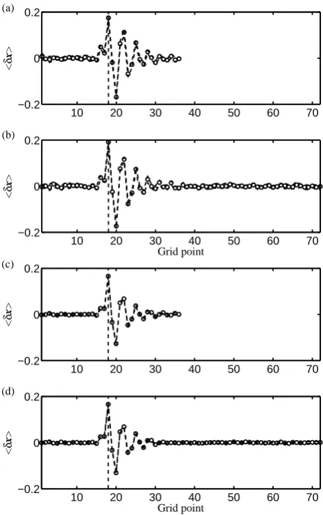
The response after a long time has elapsed of each element ofxto a continuous unit forcing applied to a single pointxk
of the Lorenz 95 system (3) is plotted in Fig. 1. The response is estimated from two long integrations of (3), withδfk=0
the right is larger in places with the amplitude reducing in a non-monotonic manner with distance. The overall impres-sion is that the response is somewhat local to the forcing and does not strongly depend upon the dimensionality ofx. In effect, the extra points in thed=72 system do not make a significant contribution to the response and we should be able to simply ignore them when making a response estimate. The experiment repeated ford=18 andd=144 does not alter this conclusion. Figure 1 suggests that the response will only be well captured if the system is truncated locally rather than in a non-local Fourier or EOF space. For the purpose of ap-plying (1), we are interested in the linear component of the response. For a forcing sufficiently small to be in the linear regime, the response to forcing more than one element ofx
may be estimated as the sum of the responses due to forcing the single elements separately. In the case of the Lorenz 95 system, all grid points are equivalent and we can calculate the response to any linear forcing by considering the response of a single grid point. In other words, the linear response to any combination ofδfj may be estimated using Fig. 1.
There-fore, we restrict ourselves to forcingδf only in the direction ofxk, so thatδfk=1 andδfj=0 forj6=k.
To investigate possible truncations, we first split the state vector into three components
x=
xk xd xi
,
wherexk is the element to which a forcing is applied,xdis
a vector of the components ofx that are closely related to
xk, andxiis a vector of the components ofxthat are in some
sense approximately independent ofxkduring an integration.
We now introduce a localised response approximation (LRA) that the PDFρk|(d,i) ofxk given a particular value of all of
the other state vector elements is equal to the PDFρk|dofxk
given only the values ofxd,
ρk|(d,i)(xk|(xd,xi))≈ρk|d(xk|xd) . (4)
This assumption is justified by the fact that changes to
ρk|(d,i)are negligible given sufficiently small variations inxi,
i.e. typical random or chaotic variations inxi are not large
enough to influence the value ofxk. The utility of the LRA
therefore depends upon the relative dimension ofxdandxi.
We use the LRA of (4) and the fact that
ρk|(d,i)(xk|(xd,xi))=
ρ (x) R
ρ (x)dxk
(5) and
ρk|d(xk|xd)= R
ρ (x)dxi R R
ρ (x)dxidxk
(6) to write
ρ (x)=ρk,d(xk,xd) ρd,i(xd,xi)
ρd(xd) , (7)
10 20 30 40 50 60 70
−0.2 0 0.2
<
δ
x
>
10 20 30 40 50 60 70
−0.2 0 0.2
Grid point
<
δ
x
>
(a)
(b)
10 20 30 40 50 60 70
−0.2 0 0.2
<
δ
x
>
10 20 30 40 50 60 70
−0.2 0 0.2
Grid point
<
δ
x
>
(c)
(d)
Fig. 1. The response hδxiof the Lorenz 95 system to a forcing of δf18=1.0 with the location of δf18 indicated by the vertical
dashed line. To compare with typical fluctuations during an inte-gration, the standard deviation of a single element ofxforδf=0 is estimated as∼3.6 fora=0. The number of elements in the state vector for (a) and (c) isd=36 and for (b) and (d) isd=72. Plots (a) and (b) correspond to the deterministic system witha=0 and (c) and (d) correspond to the same system with additional stochas-tic noise,a=2. The integrations are sufficiently long to obtain an accurate response, (2 standard deviations divided by the square root of the number of integrations is smaller than graphical accuracy), which is the same as that reported by Abramov and Majda (2007); see their Fig. 2. The difference between the first 36 points of (a) and (b) or (c) and (d) is not significantly different from zero with this set of integrations. Note that the response to linearly forcing multiple grid points simultaneously is simply the sum of the responses to the decomposed single grid point forcings.
where
ρd,i(xd,xi)= Z
ρ (x)dxk,
ρk,d(xk,xd)= Z
and
ρd(xd)= Z Z
ρ (x)dxidxk.
Substituting (7) into (1) and restricting forcing to the direc-tion ofxk, we obtain
hδx(t )i ≈ − t Z
0 D
x(τ )∂ρk,d(xk(0),xd(0)) ∂xk
1
ρk,d(xk(0),xd(0)) E
δfk(t−τ )dτ . (8)
Note that the response in the direction of xi due to δfk is
zero:
hδxi(t )i ≈0. (9)
The PDF ρk,d in (8) is a function only of xk and xd.
De-pendence uponxi has been eliminated. If we now assume
Gaussianity, we can obtain (2) for the system that involves smaller covariance matrices obtained using onlyxk andxd.
Now suppose we are interested in the response to a forcing
δf that is not restricted toδfk, we may use the fact that we
are in the linear regime to compute the linear response to forcing a single elementδfjfor eachjand sum the results.
2 A truncation algorithm
An algorithm that finds the appropriate truncation of phase space according to (8) may now be developed. We define
xr=
xk xd
.
Now we do not know in advance which elements of x to include inxd and therefore truncate iteratively towards
nu-merical convergence of our estimate of the responsehδx(t )i. Our starting point will be the maximum truncation possible, i.e. settingxrto have only the element to which the forcing
is applied, xr(t )=(xk(t )). We then obtain an estimate for
hδx(t )i using a non-parametric FDT algorithm (A1) which we denote byδxbr(t ); see Appendix A for details. Next we
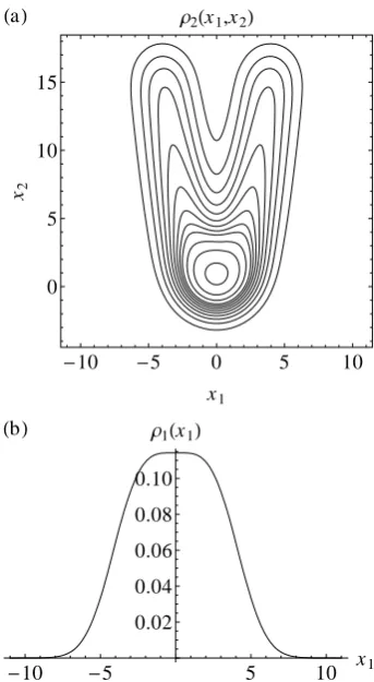
try a truncation that in addition includes another grid point and see if the estimated response of grid pointkchanges. If it does change, then using two grid points gives us a more accurate estimate ofρ (x)present in (1) and approximated in (8), see Fig. 2. On the other hand if it does not change then perhaps pointkand the tested point are independent. We re-peat this process, checking pointkwith all other grid points and pick the grid point that contributed the largest change inδxbr(t )to include in our truncated state vectorxr. For
ex-ample, if grid pointk+3 caused the estimated response to change the most, then for the next round of testing we choose
xr=
xk xk+3
.
10 5 0 5 10
0 5 10 15
x1 x2
Ρ2x1,x2 a
10 5 5 10 x1
0.02 0.04 0.06 0.08 0.10
Ρ1x1
b
Fig. 2. The contours of a two dimensional marginal PDFρ2(x1, x2)
(a). Integratingρ2(x1, x2)in thex2direction gives the one
dimen-sional marginal PDFρ1(x1)(b). In this case the plots illustrate that
the quantities∂ρ2/∂x1and∂ρ1/∂x1, which may be used in (8) are
different.
The entire process is then repeated to find the next points to add toxr, this time looking at the largest change in the
re-sponse at pointskandk+3, (estimated using the normalised root mean squared difference, RMS)
RMS distance= v u u u t
Pd0
j=1 δxbr,j(t )−δybr,j(t ) 2
Pd0
j=1 δybr,j(t )
2 ,
whereδybr,j(t )is the response estimated from the previous
round of tests and d0 indicates the current dimensionality ofxr. We continue to successively add more and more grid
points toxruntil the estimated response no longer changes.
At this point we assume that we have a good approximation of the optimal truncation so that (8) is a good approximation of (1).
One problem with our truncation algorithm is that we are comparing a response estimated using d0 grid points with a response estimated usingd0+1 grid points. Our estimate
b
δxr(t )is biased by an amount depending somehow upon the
change in the estimated response may be due to bias rather than a genuine interaction of variables. We do so by adding a variable of Gaussian distributed random numbers (with ap-proximately the same variance as that ofxk) to the truncated
state vectorxd. So in the example above we would at some
point compare the response given the vectors
xk(t ) xG(t )
and
xk(t ) xk+3(t )
,
wherexGrepresents the Gaussian random numbers. 2.1 Further truncation
It is necessary to estimate a subset of the domain to use as a starting point for the above calculation. This is because it is computationally expensive to apply the FDT to every single grid point, several times, when the number of grid points is large. One choice of region in an atmospheric context could be the set D of all points where the integral of absolute positive lagged correlations is greater than some threshold
cabs,min, i.e. the set
D=x: cabs,j(x) > cabs,min ,
for allj=1,2,3, . . . , d, where
cabs(x)=
∞
Z
0
|hx(τ )xk(0)i|dτ . (10)
Then the elements of cabsthat are greater thancabs,minwould
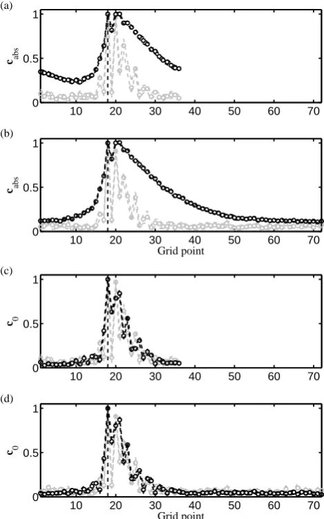
be the only points considered when looking for an appropri-ate truncation. The zero in the lower limit indicappropri-ates that we are looking for the response to a forcing, rather than all vari-ables that have some relation toxk. For the Lorenz 95 system, cabs is plotted in Fig. 3 which shows that the (normalised)
absolute value of the response lies under the (normalised) values of cabs. Note that in any suitably random system,
el-ements of cabscannot be zero because we take the absolute
value of the correlation estimate which, in turn, is subject to statistical uncertainty. Therefore, if we are able to estimate the contribution of this uncertainty, for example from two in-dependent integrations, we can pick an appropriate value for our thresholdcabs,min. For the Lorenz 95 integrations
consid-ered here the normalised value ofcabs,min∼0.12 and from
Fig. 3 we would be able to eliminate about one third of the points from the 72-element system and none of the points from the 36-element system.
Equation (10) specifies a rather conservative estimate of the region to consider and as such may not solve the prob-lem given limited computational resources. For this investi-gation, rather than cabs, a more useful truncation region is
based upon c0which is given by
c0=
∞
Z
0
hx(τ )xk(0)idτ
(11)
10 20 30 40 50 60 70
0 0.5 1
c abs
10 20 30 40 50 60 70
0 0.5 1
Grid point c abs
(a)
(b)
10 20 30 40 50 60 70
0 0.5 1
c 0
10 20 30 40 50 60 70
0 0.5 1
Grid point c 0
(c)
(d)
Fig. 3. Evaluation of (10), plots (a) and (b), and (11), plots (c) and (d), for the deterministic (a=0) Lorenz 95 system is indicated by the black lines. The grey lines indicate the absolute value of the response, |hδxi|. The number of elements in the state vector for (a) and (c) isd=36 and for (b) and (d) isd=72. The vertical scale has been normalised so thatcabs,k=c0,k= |δxk| =1 where
k=18. The location of the forcingδf18is indicated by the vertical
dashed line and statistical error, 2 standard deviations divided by the square root of the number of integrations, is smaller than graphical accuracy.
with a thresholdc0,minestimated in the same way. This is in fact the absolute value of row k of the matrix R∞
0 C(τ )dτ
consider is reduced considerably. However, to find an appro-priate threshold valuec0,min, accurate evaluation of (11) is necessary. This may not always be possible and is not such a problem for (10). Another problem with (11) is that it is only a good approximation for systems with close to Gaus-sian statistics. If a system is extremely non-GausGaus-sian, (11) may be a poor approximation and we must resort to using (10) instead.
2.2 Application of the algorithm
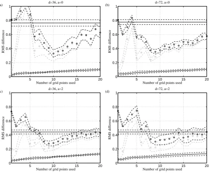
By invoking the LRA (4), we now have an algorithm that we can actually apply to high dimensional data sets provided the response to a localised forcing is sufficiently local. Using Fig. 3c and d, we consider only the region between pointsk−
7 tok+16 inclusive and apply the FDT for each truncation. The RMS difference between the true response at all grid points, (found by integrating (3)), and the response predicted by our estimation of (8) and (9) is plotted as a function of the number of elements included inxrin Fig. 4 (black circles).
Figure 4 demonstrates that for the Lorenz 95 system, pre-dictions of the response using our estimator of (8) have some skill. This figure illustrates that for a truncation to 10 grid points of the 36-element system, with the noise terma=0, the RMS error squared (i.e. the mean squared difference), is made up by variance due to a finite run length∼5 %, missing responses due to truncation∼29 % and bias in the FDT al-gorithm∼66 %. For the 36- and 72-element systems, the re-sults have similarities which indicates that for the Lorenz 95 system we may be close to the point where the predictive skill of our algorithm is independent of the dimensionality of the full state vectorx. Similar results (not shown here) were obtained with an 18-element system.
An interesting point to make about Fig. 4 is that there appears to be an optimal truncation at aroundd0=9. Un-fortunately, we did not predict the precise location of this optimum in advance. Initially the skill increases non-monotonically as more grid points are added before reach-ing the optimum truncation. The RMS error then increases slowly up to its value when all grid points are included (with-out any truncation). We can hypothesise as to the reasons be-hind this behaviour. Firstly, we have no reason to believe that high skill at predicting the response of the first point on its own would translate to other dynamical systems in some gen-eral case. Secondly, the reduction in RMS error with more than four grid points could be due to the FDT calculation in-cluding a better approximation of the underlying PDF in the manner described in Fig. 2. Thirdly, the increase in RMS er-ror beyond the optimal truncation is at least partly due to the bias present in our estimator of (8). An intuitive explanation of the cause of this bias could be simply that complex shapes present in a PDF become harder and harder to approximate accurately as their dimensionality increases. In our case we are approximating the underlying PDF by a convolution of the data (from integrations) with a kernel function; see
Ap-pendix A. As the dimensionalityd0of phase space increases, the integral over all xr of the kernel function must remain
constant. Fixing an acceptable level of variance in the pre-dictions of the FDT and increasing the dimensionality has the effect of requiring a broader kernel to approximate the PDF with. Eventually, the kernel is so broad that one may as well approximate the convolution of the data and the kernel with a single Gaussian blob with non-isotropic covariance. If this is true for our system then the response predicted by the Gaussian form of the FDT (2) and Eq. (1) using our estima-tor, should be approximately the same; see Fig. 5.
The fact that our estimator approximates a smoothing con-volution of the PDF leads us to suspect that it has skill when applied to stochastic systems where the white noise term leads to a genuinely smooth underlying PDF. Although it may appear slight, the FDT (A1) has more skill for the stochastic case wherea=2 than the deterministic case wherea=0; see Fig. 4. Given sufficient smoothing (by in-creasing the value ofa), we eventually get to the situation where the non-Gaussian aspects of the underlying PDF are small corrections to ad0dimensional Gaussian. In this case the Gaussian approximation (2) is a good one.
3 Conclusions
If we wish to apply the fluctuation-dissipation theorem (FDT) to predict the response to forcing in general circula-tion models, reanalysis data sets, and measurements of the climate system, truncation of the huge state vector present in these systems seems necessary. We have argued that trun-cation of the state vector to include only the locality of the forcing (according to variations in predictions of the FDT) may be appropriate to some chaotic high dimensional sys-tems and have tested this hypothesis using a 36- and 72-element Lorenz 95 system. The practical implications of this localised response approximation (LRA) are, for example, that if we consider the atmospheric response to a heating over one small part of the planet, perhaps there are regions that contribute very little to the response. If these regions ex-ist then they may be safely ignored in a FDT calculation.
5 10 15 20 0
0.2 0.4 0.6 0.8 1
RMS difference
d=36, a=0
Number of grid points used (a)
5 10 15 20
0 0.2 0.4 0.6 0.8 1
Number of grid points used
RMS difference
d=72, a=0 (b)
5 10 15 20
0 0.2 0.4 0.6 0.8 1
Number of grid points used
RMS difference
d=36, a=2 (c)
5 10 15 20
0 0.2 0.4 0.6 0.8 1
Number of grid points used
RMS difference
d=72, a=2 (d)
Fig. 4. RMS difference between the response of the Lorenz 95 system estimated by integrating (3) and using the non-parametric FDT (A1) where the number of elements in the full state vector for (a) and (c) isd= 36and for (b) and (d) isd= 72. Plots (a) and (b) correspond to the deterministic system witha= 0and plots (c) and (d) correspond to the same system with additional stochastic noise,a= 2. The black circles indicate the RMS difference of the entire state vector using (8) and (9). The grey circles indicate the RMS difference of only the elements to which the calculation is applied using (8). The solid line at the bottom of each plot indicates the minimum possible RMS difference of the grey circles with this data set. I.e. the difference between the responses estimated using two independent sets of data found by integrating (3). The straight horizontal line is the RMS difference between integrating (3) and the response estimated using the Gaussian form of the FDT (2) for the 36 element system, see figure (5) for a plot of this response. The dashed lines, indicating uncertainty, represent two standard deviations divided by the square root of the number of independent integrations. An estimate with zero skill, (given by (9) with the entire state vector being independent of the forcing), has a RMS difference of one using this normalisation. It is possible to do worse than this by overestimating the response by a factor of greater than 2.
The FDT applied here gives only the linear component of the response of the non-linear system considered. This is a good approximation for the full response if the forcing is suf-ficiently small. Being linear, the sum of the responses esti-mated separately for two different forcings is identical to the single response estimated for the sum of these two forcings. We may therefore estimate the entire set of possible linear re-sponses by appropriate summing of the rere-sponses to forcing
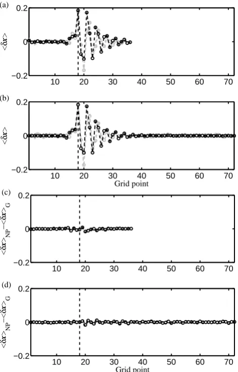
each grid point individually. Similarly, quantities such as the response in the mean, or any other combination of several variables, may be estimated from the appropriate combina-tion of responses to separate local forcings. Forcings suffi-ciently large to make the response strongly non-linear are in general not susceptible to any simple linear decomposition into localised forcings. In addition (1) only applies to the lin-ear component of any response calculation and large forcings Fig. 4. RMS difference between the response of the Lorenz 95 system estimated by integrating (3) and using the non-parametric FDT (A1) where the number of elements in the full state vector for (a) and (c) isd=36 and for (b) and (d) isd=72. Plots (a) and (b) correspond to the deterministic system witha=0 and plots (c) and (d) correspond to the same system with additional stochastic noise,a=2. The black circles indicate the RMS difference of the entire state vector using (8) and (9). The grey circles indicate the RMS difference of only the elements to which the calculation is applied using (8). The solid line at the bottom of each plot indicates the minimum possible RMS difference of the grey circles with this data set, i.e. the difference between the responses estimated using two independent sets of data found by integrating (3). The straight horizontal line is the RMS difference between integrating (3) and the response estimated using the Gaussian form of the FDT (2) for the 36-element system; see Fig. (5) for a plot of this response. The dashed lines, indicating uncertainty, represent two standard deviations divided by the square root of the number of independent integrations. An estimate with zero skill, (given by (9) with the entire state vector being independent of the forcing), has a RMS difference of one using this normalisation. It is possible to do worse than this by overestimating the response by a factor of greater than 2.
The FDT applied here gives only the linear component of the response of the non-linear system considered. This is a good approximation for the full response if the forcing is sufficiently small. Being linear, the sum of the responses esti-mated separately for two different forcings is identical to the single response estimated for the sum of these two forcings. We may therefore estimate the entire set of possible linear re-sponses by appropriate summing of the rere-sponses to forcing each grid point individually. Similarly, quantities such as the response in the mean, or any other combination of several variables, may be estimated from the appropriate combina-tion of responses to separate local forcings. Forcings suffi-ciently large to make the response strongly non-linear are in
general not susceptible to any simple linear decomposition into localised forcings. In addition (1) only applies to the lin-ear component of any response calculation and large forcings require a generalisation (e.g. Boffetta et al., 2003). In some situations, even with simple systems similar to that consid-ered here, the response may be entirely non-linear (Lacorata and Vulpiani, 2007).
10 20 30 40 50 60 70 −0.2
0 0.2
<
δ
x
>
10 20 30 40 50 60 70
−0.2 0 0.2
Grid point
<
δ
x
>
(a)
(b)
10 20 30 40 50 60 70
−0.2 0 0.2
<
δ
x
> NP
−<
δ
x
> G
10 20 30 40 50 60 70
−0.2 0 0.2
Grid point
<
δ
x
> NP
−<
δ
x
> G (c)
(d)
Fig. 5. Response of the deterministic (a=0) Lorenz 95 system es-timated using the Gaussian FDT (2), plots (a) and (b), and the dif-ference between the Gaussian FDT (2) and the non-parametric FDT (A1) as an estimator of (1) without truncation, plots (c) and (d). The number of elements in the state vector for (a) and (c) isd=36 and for (b) and (d) isd=72. The grey lines indicate the true response plotted in Fig. 1 and the RMS difference between the grey and black points is∼75 % as indicated by the uppermost straight horizontal lines in Fig. 4. The location of the forcingδf18is indicated by the
vertical dashed line and statistical error, 2 standard deviations di-vided by the square root of the number of integrations, is smaller than graphical accuracy.
necessarily increases the width of the kernel function relative to the distance between data points leading to a worse PDF approximation. In a high dimensional space, the kernel func-tions significantly overlap and although we have not shown it in any analytical way, the non-parametric FDT seems to ap-proach the Gaussian FDT (Fig. 5). If the response to a local forcing is spread over a large number of grid points (and an accurate transformation to a smaller number of grid points is not available), then the dimensionality of phase space in which the non-parametric FDT must approximate a PDF is
also large. If the PDF has a complex shape then its accurate approximation is extremely difficult and is likely to require more data than is possible to obtain. Deterministic systems may even have a fractal PDF that makes use of (1) difficult to justify. Other expressions such as the linear response rela-tion of Ruelle (1998) may have to be considered.
In addition to using truncation, there are several improve-ments that could be made to the non-parametric FDT algo-rithm. It may be possible to obtain insight into its bias by considering different kernels with the same data set, or to re-duce the bias via adaptive density estimation, see Silverman (1986) and Cooper and Haynes (2011). If restrictions such as conservation laws can be placed upon a system’s PDF, per-haps by analytical consideration of the underlying equations, it may also be easier to approximate. Another approach may be to adopt the tangent linear algorithm of Eyink et al. (2004) with the “blended response” modification of Abramov and Majda (2007) which replaces estimation of the PDF by esti-mation (or calculation if the underlying equations are avail-able) of a tangent linear system.
Appendix A
Experiment specification
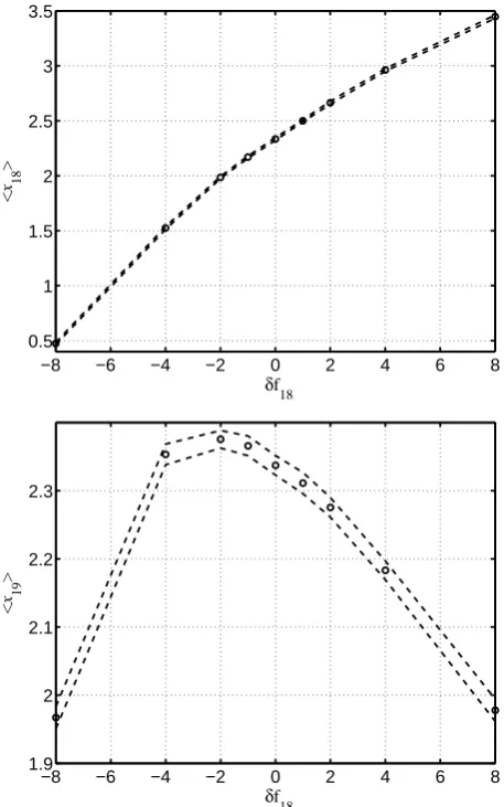
We test the FDT (1) using the stochastic Lorenz 95 sys-tem introduced above where we choose the constantf =8. It is approximated by applying a fourth-order Runge–Kutta method (Press et al., 2002) to the deterministic part of (3) and the method of R¨umelin (R¨umelin, 1982) to the stochas-tic part using the Mersenne Twister algorithm (Matsumoto and Nishimura, 1998) for random numbers. We choose state vectors of sized=36 andd=72 and starting with random initial conditions we use a time step of 1t=10−3 and af-ter discarding 105 time steps iterate fromt=0 tot=106. This may be compared with∼1.74, the value of the largest Lyapunov exponent for the deterministic system (Abramov and Majda, 2007). We perform 10 identically specified inte-grations with different initial conditions for each experiment in order to get a measure of the statistical uncertainty. Equa-tion (8) is only valid in the linear regime, i.e. for a sufficiently small forcing. In order to discover the range over which the linear approximation is valid, we perform several integra-tions of (3) with −8≤δfk≤8 andδfj=0 for j6=k and
k=18. The average value of elements 18 and 19 of the state vector of thed=36,a=0 integrations averaged over 1010 time steps is plotted in Fig. A1. For a forcing ofδf18= ±1
the non-linear component of the response is small in compar-ison with the size of the total response. A similar range and accuracy of linearity is observed for all elements of the state vector, and if the integrations are carried out withd=72.
−8 −6 −4 −2 0 2 4 6 8 0.5
1 1.5 2 2.5 3 3.5
<
x 18
>
δf
18
−8 −6 −4 −2 0 2 4 6 8
1.9 2 2.1 2.2 2.3
<
x 19
>
δf 18
Fig. A1. The mean value of state vector elementx18andx19 of a
36-element Lorenz 95 system as a function of forcing applied to x18 to illustrate the range of linearity of the response. The dashed
lines indicate two standard deviations divided by the square root of the number of independent integrations (of which there are 10). Plots of the response of other vector elements or of the elements of a 72-element or stochastic Lorenz 95 system yield similar ranges of linearity with different gradients near the origin.
the standard unbiased estimator for the covariance C(τ ). Fol-lowing Cooper and Haynes (2011), we approximate (8) by the non-parametric method
ˆ
3(s1t )= m X j=1
Xj+s " Pn
i=1 Xj−Xi T
E Xj;Xi, h h2Pn
i=1E Xj;Xi, h #
and
b δx(h)=
r X
s=0
µs3(ˆ 0)−13(s1t ) δfˆ , (A1)
whereδx(h)b is the estimated response as a function of the
free parameter h andX is the appropriate segment of the
state vector recorded at a particular time. Here a unit of the indicesiandj correspond to a time between recordings of
Xof 10 and a unit of the indexscorresponds to a time be-tween recordings of 10−3. So for example ifi=5,j=7 and
s=137 then the values oft that Xi,Xj andXj+s
corre-spond to are 50, 70 and 70.137, respectively. To evaluate (A1) we user=104 (representing 10 time units to approximate infinity as the upper limit of the integral in (8)),m=105,
n=105,µ0=0.51tandµs=1tfors >0 with our choice
being motivated by a trade off between accuracy and avail-able computational power; see Cooper and Haynes (2011). In Cooper and Haynes (2011), the function E was repre-sented byN, addimensional Gaussian with isotropic covari-anceh. Here for computational efficiency we use the multi-dimensional Epanechnikov kernel (Silverman, 1986) with-out normalisation
E (x;y, h)= (
h2−(x−y)T(x−y) , |x−y|< h
0, otherwise.
(A2) To estimate the response using (A1), a value of the free pa-rameterhmust be chosen. We choose the smallest guess ofh
that corresponds to the standard deviation of the estimated re-sponse of elementx18being no larger than five percent of the estimate of its mean. Our choice ofhis not well optimised because this is computationally expensive and the benefits of improving upon a simple guess appear small; see Cooper and Haynes (2011) for a discussion.
Acknowledgements. Thanks go to H. Salman for useful discus-sions. This research was supported by the Natural Environment Research Council Grant NE/G003122/1 to J. G. Esler and by the EU funded SHIVA project.
Edited by: O. Talagrand
Reviewed by: two anonymous referees
References
Abramov, R. V. and Majda, A. J.: Blended response algorithms for linear fluctuation-dissipation for complex nonlinear dynam-ical systems, Nonlinearity, 20, 2793–2821, doi:10.1088/0951-7715/20/12/004, 2007.
Boffetta, G., Lacorata, G., Musacchio, S., and Vulpiani, A.: Relax-ation of finite perturbRelax-ations: Beyond the fluctuRelax-ation-response re-lation, Chaos, 13, 806–811, doi:10.1063/1.1579643, 2003. Cooper, F. C. and Haynes, P. H.: Climate Sensitivity via a
Non-parametric Fluctuation-Dissipation Theorem, J. Atmos. Sci., 68, 937–953, doi:10.1175/2010JAS3633.1, 2011.
Davies, T., Cullen, M. J. P., Malcolm, A. J., Mawson, M. H., Stani-forth, A., White, A., and Wood, N.: A new dynamical core for the Met Office’s global and regional modelling of the atmosphere, Q. J. Roy. Meteor. Soc., 131, 1759–1782, doi:10.1256/qj.04.101, 2005.
Eyink, G. L., Haine, T. W. N., and Lea, D. J.: Ruelle’s linear response formula, ensemble adjoint schemes and L´evy flights, Nonlinearity, 17, 1867–1889, doi:10.1088/0951-7715/17/5/016, 2004.
Gritsun, A. and Branstator, G.: Climate Response Using a Three-Dimensional Operator Based on the Fluctuation-Dissipation Theorem, J. Atmos. Sci., 64, 2558–2575, doi:10.1175/JAS3943.1, 2007.
Joliffe, I. T.: Principal Component Analysis, Springer Series in Statistics, 2nd Edn., 2002.
Lacorata, G. and Vulpiani, A.: Fluctuation-Response Relation and modeling in systems with fast and slow dynamics, Nonlin. Pro-cesses Geophys., 14, 681–694, doi:10.5194/npg-14-681-2007, 2007.
Lorenz, E. N.: Predictability: a problem partly solved, Proceed-ings from the ECMWF Seminar on Predictability, volume Vol. I, ECMWF, Reading, UK, 1995.
Lucarini, V. and Sarno, S.: A statistical mechanical approach for the computation of the climatic response to general forcings, Non-lin. Processes Geophys., 18, 7–28, doi:10.5194/npg-18-7-2011, 2011.
Majda, A. J., Gershgorin, B., and Yuan, Y.: Low-Frequency Climate Response and Fluctuation-Dissipation Theo-rems: Theory and Practice, J. Atmos. Sci., 67, 1186–1201, doi:10.1175/2009JAS3264.1, 2010.
Marconi, U. M. B., Puglisi, A., Rondoni, L., and Vulpi-ani, A.: Fluctuation-dissipation: Response theory in statistical physics, Physics Reports, 461, 111–195, doi:10.1016/j.physrep.2008.02.002, 2008.
Matsumoto, M. and Nishimura, T.: Mersenne Twister: A 623-dimensionally equidistributed uniform pseudorandom number generator, ACM T. Model. Comput. S., 8, 3–30, 1998.
Press, W. H., Teukolsky, S. A., Vetterling, W. T., and Flannery, B. P.: Numerical Recipes in C++: The Art of Scientific Computing, Cambridge University Press, UK, 2002.
Ring, M. and Plumb, R. A.: The Response of a Simpli-fied GCM to Axisymmetric Forcings: Applicability of the Fluctuation-Dissipation Theorem, J. Atmos. Sci., 65, 3880– 3898, doio:10.1175/2008JAS2773.1, 2008.
Ruelle, D.: General linear response formula in statistical me-chanics, and the fluctuation-dissipation theorem far from equi-librium, Phys. Lett. A, 245, 220–224, doi:10.1016/S0375-9601(98)00419-8, 1998.
R¨umelin, W.: Numerical Treatment of Stochastic Differential Equa-tions, SIAM J. Numer. Anal., 19, 604–613, 1982.