Shengli Chen, Daoyi Chen, and Jiuxing Xing
Shenzhen Key Laboratory for Coastal Ocean Dynamic and Environment, Graduate School at Shenzhen, Tsinghua University, Shenzhen 518055, China
Correspondence to:Jiuxing Xing ([email protected]) Received: 5 May 2017 – Discussion started: 31 May 2017
Revised: 8 September 2017 – Accepted: 12 September 2017 – Published: 17 October 2017
Abstract. Some basic features of inertial oscillations and near-inertial internal waves are investigated by simulating a two-dimensional (x−z) rectangular basin (300 km×60 m) driven by a wind pulse. For the homogeneous case, near-inertial motions are pure near-inertial oscillations. The near-inertial os-cillation shows typical opposite currents between the surface and lower layers, which is formed by the feedback between barotropic waves and inertial currents. For the stratified case, near-inertial internal waves are generated at land boundaries and propagate offshore with higher frequencies, which in-duce tilting of velocity contours in the thermocline. The iner-tial oscillation is uniform across the whole basin, except near the coastal boundaries (∼20 km), where it quickly declines to zero. This boundary effect is related to great enhance-ment of non-linear terms, especially the vertical non-linear term (w∂u/∂z). With the inclusion of near-inertial internal waves, the total near-inertial energy has a slight change, with the occurrence of a small peak at ∼50 km, which is simi-lar to previous research. We conclude that, for this distribu-tion of near-inertial energy, the boundary effect for inertial oscillations is primary, and the near-inertial internal wave plays a secondary role. Homogeneous cases with various wa-ter depths (50, 40, 30, and 20 m) are also simulated. It is found that near-inertial energy monotonously declines with decreasing water depth, because more energy of the initial wind-driven currents is transferred to seiches by barotropic waves. For the case of 20 m, the seiche energy even slightly exceeds the near-inertial energy. We suppose this is an im-portant reason why near-inertial motions are weak and hardly observed in coastal regions.
1 Introduction
Near-inertial motions have been observed and reported in many seas (e.g. Alford et al., 2016; Webster, 1968). They are mainly generated by changing winds at the sea surface (Pol-lard and Mil(Pol-lard, 1970; Chen et al., 2015b). The passage of a cyclone or a front can induce strong near-inertial motions (D’Asaro, 1985), which can last for 1–2 weeks and reach a maximum velocity magnitude of 0.5–1.0 m s−1(Chen et al., 2015a; Zheng et al., 2006; Sun et al., 2011). In deep seas, the near-inertial internal wave propagates downwards to trans-fer energy to depth (Leaman and Sanford, 1975; Fu, 1981; Gill, 1984; Alford et al., 2012). The strong vertical shear of near-inertial currents may play an important role in inducing mixing across the thermocline (Price, 1981; Burchard and Rippeth, 2009; Chen et al., 2016).
In shelf seas, near-inertial motions exhibit a two-layer structure, with an opposite phase between currents in the surface and lower layers (Malone, 1968; Millot and Crepon, 1981; MacKinnon and Gregg, 2005). By solving a two-layer analytic model using the Laplace transform, Pettigrew (1981) found this “baroclinic” structure can be formed by inertial oscillations without inclusion of near-inertial internal waves. Due to similar vertical structures and frequencies, inertial os-cillations and near-inertial internal waves are hardly separa-ble, and could easily be mistaken for each other.
verti-Figure 1.Velocities (uandv, m s−1) atx=70 km. The white lines denote the value of zero. The contour interval is 0.02 m s−1for both panels.
Figure 2. Snapshots of eastward velocity and elevation (η) at
t=0.5 and 1 h. The white lines represent the value of zero.
cal gradient of Reynolds stress near the shelf break. By using the analytic model of Pettigrew (1981), Shearman (2005) ar-gued that the cross-shelf variation is controlled by baroclinic waves which emanate from the coast to introduce nullifying effects on the near-inertial energy near the shore. Kundu et al. (1983) found a coastal inhibition of near-inertial energy within the Rossby radius from the coast, which is attributed to leaking of near-inertial energy downward and offshore. As many factors seem to work, the mechanism controlling the cross-shelf variation of near-inertial energy is not clear.
In this paper, simple two-dimensional simulations are used to investigate some basic features of near-inertial motions. Cases with and without vertical stratification are simulated to examine properties and differences between inertial oscil-lations and near-inertial internal waves. The horizontal dis-tribution of near-inertial energy is discussed in detail. Also, cases with various water depths are simulated to investigate the dependence of near-inertial motions on the water depth.
Figure 3. (a)Time series of velocities and elevation atx=100 km. “v0” and “v40” mean the northward velocity (v)at depths of 0 and 40 m, and “u40” is the eastward velocity (u)at 40 m.(b)Contours ofvatx=100 km. The white lines denote the value of zero, and the contour interval is 0.02 m s−1.
2 Model settings
The simulated region is a two-dimensional shallow rectangu-lar basin (300 km×60 m). Numerical simulations are done by the MIT general circulation model (MITgcm; Marshall et al., 1997), which discretizes the primitive equations and can be designed to model a wide range of phenomena. There are 1500 grid points in the horizontal (1x=200 m) and 60 grid points in the vertical (1z=1 m). The water depth is uniform, with the eastern and western sides being land boundaries. The vertical and horizontal eddy viscosities are assumed con-stant as 5×10⁻⁴and 10 m2s−1, respectively. The Coriolis parameter is 5×10⁻⁵s−1 (at a latitude of 20.11◦N). The bottom boundary is non-slip. The model is forced by a spa-tially uniform wind which is kept westward and increases from 0 to 0.73 N m−2 (corresponding to a wind speed of 20 m s−1) for the first 3 h and then suddenly stops. The model runs for 200 h in total, with a time step of 4 s. The first case is homogeneous, while the second one has a stratification of a two-layer structure initially. For the stratified case, the tem-perature is 20◦C in the upper layer (−30 m < z < 0) and 15◦C in the lower layer (−60 m < z <−30 m). The salinity is con-stant, and the density is linearly determined by the temper-ature, with an expansion coefficient of 2×10⁻⁴◦C−1. The barotropic and baroclinic Rossby radii are 485 and 8 km, re-spectively.
3 Inertial oscillations
Figure 4. Time series of the northward velocity (v) at different depths and positions. “v0” and “v40” mean vat depths of 0 and 40 m.
3.1 Vertical structures
The model simulated velocities (Fig. 1) vary near the iner-tial period (34.9 h). Spectra of velocities (not shown) indicate maximum peaks located exactly at the inertial period. The spectra ofualso have a smaller peak at the period of the first mode seiche (6.9 h). As this simulation is two-dimensional, i.e. the gradient along the y-axis is zero, the u/v of se-iches have a value of ωn/f (equals 5 for the first mode se-iche). Thus there is little energy of seiches inv, which shows clearly regular variation at the inertial frequency.
In the vertical direction, currents display a two-layer struc-ture, with their phase being opposite between the surface and lower layers. They are maximum at the surface, and have a weaker maximum in the lower layer (∼40 m), with a minimum at a depth of∼20 m. The velocity gradually di-minishes to zero at the bottom due to the bottom friction. This is the typical vertical structure of shelf sea inertial os-cillations, which have been frequently observed (Shearman, 2005; MacKinnon and Gregg, 2005). In practice, this verti-cal distribution can be modified due to the presence of other processes, such as the surface maximum being pushed down to the subsurface (e.g. Chen et al., 2015a). Note that without stratification in this simulation the near-inertial internal wave is absent. However, this two-layer structure of inertial oscil-lations looks ‘baroclinic’, which makes it easy to be mistak-enly attributed to the near-inertial internal wave (Pettigrew, 1981).
It is interesting that currents of non-baroclinic inertial os-cillations reverse between the surface and lower layers. This is usually due to the presence of the coast, which requires the normal-to-coast transport to be zero; thus, currents in the
up-Figure 6.Variation of depth-mean inertial and non-linear terms (m s−2). The inertial term(a)is calculated as|f (u+iv)|, the hor-izontal non-linear term(b)is|u (∂u/∂x+i∂v/∂x)|, and the verti-cal non-linear term(c)is|w (∂u/∂z+i∂v/∂z)|.(d)Time-averaged value for the first 50 h.
per and lower layers compensate each other (e.g. Millot and Crepon, 1981; Chen et al., 1996). However, it is interesting to see how this vertical structure is established step by step.
iner-Figure 7.Snapshots of temperature profiles att=20, 40, 80, and 120 h. The contour interval is 0.5◦C.
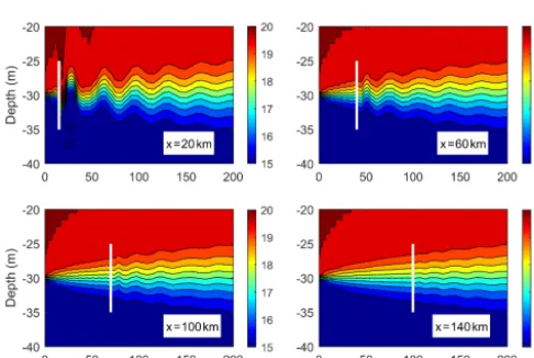
Figure 8. Time series of temperature at x=20, 60, 100, and 140 km. White lines denote the arrival of internal waves. The con-tour interval is 0.5◦C.
tial currents in the surface and lower layers having opposite directions and comparable amplitudes. As seen from Fig. 1b, the typical vertical structure of inertial currents is established within the first inertial period.
3.2 Horizontal distributions of inertial energy
The inertial velocities are almost entirely the same across the basin (Fig. 4), except near the land boundaries. This indi-cates that inertial oscillations have a coherence scale of al-most the basin width. This is because in our simulation the wind force is spatially uniform, and the bottom is flat. The inertial velocities in the lower layer have slightly more varia-tion across the basin than those in the surface layer, because inertial velocities in the lower layer depend on the propaga-tion of barotropic waves as discussed in Sect. 3.1, while the surface inertial currents are driven by spatially uniform wind. In shelf sea regions, the wind forcing is usually coherent as the synoptic scale is much larger; however, the topography
Figure 9. (a)Spectra of the temperature at the mid-depth (z= −30 m). The pink dashed line represents the inertial frequency. (b)Sum of spectra in the inertial band with a red line denoting the e-folding value of the peak.(c)Theoretical spectra of mid-depth elevation calculated from the solution in the form of a Bessel func-tion as in Eq. (3.16) of Pettigrew (1981).(d)Same as(b)but for theoretical spectra.
Figure 10.Distribution of near-inertial currents (v, m s−1) and cur-rent spirals for the cases without (a,b,c) and with (d,e,f) strat-ification atx=30 km. The near-inertial currents are obtained by applying a band-pass filter. The contour interval is 0.02 m s−1.
that is mostly not flat could generate barotropic waves at var-ious places and thus significantly decrease coherence of in-ertial currents in the lower layer.
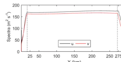
The spectra of velocities in the inertial band are almost uniform except near the land boundaries (Fig. 5), consistent with the velocities. Near the boundaries, the inertial energy declines gradually to zero fromx=∼20 km to the land. The eastern side has slightly greater inertial energy and a slightly wider boundary layer compared to the western side.
boundary (Fig. 6bc), where the inertial term is weak (Fig. 6a). For the time-averaged values (Fig. 6d), the vertical non-linear term is 2 times more than the horizontal non-linear term. The inertial term drops sharply near the boundary, and rises grad-ually with distance away from the boundary. Atx> 15 km, it keeps an almost constant value which is much greater than non-linear terms. Thus it is concluded that the significant decrease in inertial oscillations near the boundary is due to the influence of linear terms, especially the vertical non-linear term.
4 Near-inertial internal waves
In addition to inertial oscillations, near-inertial internal waves are usually generated when the vertical stratification is present. However, due to their close frequencies, inertial os-cillations and near-inertial internal waves are difficult to sep-arate. Thus we run a second simulation with the presence of stratification to investigate the differences that near-inertial internal waves introduce.
4.1 Temperature distributions
Figure 7 shows the evolution of temperature profiles with time. One can see an internal wave packet is generated at the western coast and then propagates offshore. The wave phase speed is about 1 km h−1, close to the theoretical value (1.4 km h−1). Before the arrival of internal waves, the tem-perature at mid-depth diffuses gradually due to vertical diffu-sion in the model. For a fixed position atx=20 km (Fig. 8), the temperature varies with the inertial period (34.9 h) and the amplitude of fluctuation declines gradually with time. At
x=60 km and x=100 km, the strength of internal waves is much reduced, and wave periods are shorter initially, followed by a gradual increase to the inertial period. At
x=140 km, the internal wave becomes as weak as the back-ground disturbance.
A spectral analysis of the temperature at mid-depth (z= −30 m) is shown in Fig. 9a. The strongest peak is near the inertial frequency (0.69 cpd), but is only confined to the region close to the boundary (x< 40 km). In the region 20 km <x< 70 km, the energy is also large at higher
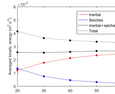
fre-Figure 12.The kinetic energy of near-inertial motions and seiches for different water depths. For each case, the currents are band-pass filtered to get currents for each type of motion which are then aver-aged over time and integrated over space to obtain a final value.
quencies of 0.8–1.7 cpd. This generally agrees with prop-erties of Poincaré waves. During Rossby adjustment, the waves with higher frequencies propagate offshore at greater group speeds; thus, for places further offshore, the waves have higher frequencies (Millot and Crepon, 1981), while the wave with a frequency closest to the inertial frequency moves at the slowest group velocity, and it takes a relatively long time to propagate far offshore; thus, it is mostly con-fined to near the boundary. By solving an idealized two-layer model equation, the response of Rossby adjustment can be expressed in the form of Bessel functions (Millot and Cre-pon, 1981; Gill, 1982; Pettigrew, 1981), as in Fig. 9cd show-ing the spectra of mid-depth elevation. The difference from our case is obvious. The frequency of theoretical near-inertial waves increases gradually with distance from the coast, while in our case this property is absent. And the theoretical iner-tial energy has ane-folding scale of 54 km, while in our case thee-folding scale is much smaller (∼15 km).
4.2 Velocity distributions
With the presence of near-inertial internal waves, the contours of velocities near the thermocline tilt slightly (Fig. 10d), and indicate an upward propagation of phase and thus a downward energy flux. This can also be seen in ver-tical spirals of velocities (Fig. 10e and f). With only inertial oscillations, current vectors mostly point toward two oppo-site directions (Fig. 10b and c). Once the near-inertial wave is included, the current vectors gradually rotate clockwise with depth.
Figure 13.Vertical profile of averaged inertial kinetic energy for the homogeneous cases with water depths of 20, 40, and 60 m. The red dashed line in(c)denotes the slip case.
energy reaches a peak. Further away (> 100 km) it becomes a constant. This spatial distribution of inertial energy is similar to that observed in shelf seas, with a maximum near the shelf break (Chen et al., 1996; Shearman, 2005). In our case, the boundary layer effect which induces a sharp decrease to zero makes a major contribution, and near-inertial internal waves which bring a small peak further offshore have a secondary influence.
5 Dependence on the water depth
In coastal regions, near-inertial motions are rarely reported. It is speculated that the strong dissipation and bottom friction in coastal regions suppress the development of near-inertial motions. However, Chen (2014) found the water depth is also a sensitive factor, with significant reduction for the case with smaller water depth. Here we will run cases with different water depths and clarify why the near-inertial energy changes with water depth. Homogeneous cases with water depths of 50, 40, 30, and 20 m are simulated. The vertical model reso-lution for all cases is 1 m. All the other parameters including viscosities are the same as the homogeneous case of 60 m.
For each case, the currents are band-pass filtered to ob-tain near-inertial currents. Then near-inertial kinetic energy can be calculated. As seen in Fig. 12, the near-inertial en-ergy gradually declines with decreasing water depth. In this dynamical system, the other dominant process is the seiche induced by barotropic waves. As the elevation induced by seiches is anti-symmetric in such a basin, the potential en-ergy is little. The kinetic enen-ergy of seiches can also be calcu-lated by the band-pass filtered currents. We find the energy of seiches, by contrast, increases gradually with decreasing water depth. For the case of 60 m, the near-inertial energy is much greater than the seiche energy. But for the case of 20 m, the energy of seiches has exceeded the near-inertial energy slightly. The total energy of these two processes almost stays constant for all cases. For a shallower water depth, the
re-than 30 m, the near-inertial motion is weak, due to the sup-pression of barotropic waves.
As seen in Sect. 3.1, inertial oscillations behave in a two-layer structure, with currents in the upper two-layer in opposite phase with those of the lower layer. In terms of kinetic en-ergy, for the case of 60 m (Fig. 13), the near-inertial motion is maximized in the surface, minimized near the depth of 20 m, and then gradually increases with depth to form a much smaller peak at 40 m. Near the bottom, the near-inertial en-ergy gradually reduces to zero due to bottom friction. When we set the bottom boundary condition from non-slip to slip, such a boundary structure vanishes, and near-inertial energy becomes constant in the lower layer. For the other cases of 20 and 40 m, their vertical profiles are almost the same as the 60 m case. The minimum positions are all located at 1/3 of the water depth. This implies the vertical distribution of near-inertial energy is independent of water depth. Note that in our cases the vertical viscosity is set as a constant value. In practice, the viscosity in the thermocline is usually signif-icantly reduced; thus, the minimum position of near-inertial energy is located just below the mixed layer.
6 Summary and discussion
examine the occurrence of near-inertial internal waves. Near the land boundary the vertical elevation generates fluctua-tions of the thermocline that propagate offshore. The en-ergy of near-inertial internal waves is confined to near the land boundary (x< 40 km). At positions further offshore, the waves have higher frequencies. This is generally consistent with properties of a Rossby adjustment process. However, our simulated results also show evident discrepancies with theoretical values obtained in the classic solutions of the Rossby adjustment problem. These discrepancies are proba-bly due to non-linearity of the model and the changing strat-ification in the model due to diffusion and mixing, compared to constant density differences between the two layers in the-oretical cases.
The inertial oscillation has a very large coherent scale of almost the whole basin scale. It is uniform in both am-plitude and phase across the basin, except near the bound-ary (∼20 km offshore). The energy of inertial oscillations declines gradually to zero from x=20 km to the coast. This boundary effect is attributed to the influence of non-linear terms, especially the vertical term (w∂u/∂z), which is greatly enhanced near the boundary and overweighs the iner-tial term (fu). When near-inertial internal waves are pro-duced in the stratified case, the distribution of total near-inertial energy is modified slightly near the boundary. A small peak appears at ∼50 km offshore. This is similar to the cross-shelf distribution of near-inertial energy observed in shelf seas (Chen et al., 1996; Shearman, 2005). This en-ergy distribution has been attributed to downward and off-shore leakage of near-inertial energy near the coast (Kundu et al., 1983), the variation of elevation and Reynolds stress terms associated with the topography (Chen and Xie, 1997), and the influence of the baroclinic wave (Shearman, 2005; Nicholls et al., 2012). In our simulations, this horizontal dis-tribution of near-inertial energy is primarily controlled by the boundary effect on inertial oscillations, and the near-inertial internal wave has a secondary effect.
Homogeneous cases with various water depths (50, 40, 30, and 20 m) are also simulated. The inertial energy is reduced with decreasing water depth, while the energy of seiches, by contrast, is increased. For the case of 20 m, the seiche energy slightly exceeds the inertial energy. It is interesting that the reduction of inertial energy just equals the increase in the
of interest.
Acknowledgements. We are grateful for discussions with John Huthnance and comments from the editor and reviewers. This study is supported by the National Basic Research Pro-gram of China (2014CB745002, 2015CB954004), the Shenzhen government (201510150880, SZHY2014-B01-001), and the Natural Science Foundation of China (U1405233). Shengli Chen is sponsored by the China Postdoctoral Science Foundation (2016M591159).
Edited by: Neil Wells
Reviewed by: two anonymous referees
References
Alford, M. H., Cronin, M. F., and Klymak, J. M.: Annual Cycle and Depth Penetration of Wind-Generated Near-Inertial Internal Waves at Ocean Station Papa in the Northeast Pacific, J. Phys. Oceanogr., 42, 889–909, https://doi.org/10.1175/jpo-d-11-092.1, 2012.
Alford, M. H., MacKinnon, J. A., Simmons, H. L., and Nash, J. D.: Near-Inertial Internal Gravity Waves in the Ocean, Ann. Rev. Mar. Sci., 8, 95–123, https://doi.org/10.1146/annurev-marine-010814-015746, 2016.
Burchard, H. and Rippeth, T. P.: Generation of Bulk Shear Spikes in Shallow Stratified Tidal Seas, J. Phys. Oceanogr., 39, 969–985, 10.1175/2008jpo4074.1, 2009.
Chen, C. and Xie, L.: A numerical study of wind-induced, near-inertial oscillations over the Texas-Louisiana shelf, J. Geophys. Res.-Oceans, 102, 15583–15593, https://doi.org/10.1029/97jc00228, 1997.
Chen, C. S., Reid, R. O., and Nowlin, W. D.: Near-inertial oscilla-tions over the Texas Louisiana shelf, J. Geophys. Res.-Oceans, 101, 3509–3524, https://doi.org/10.1029/95jc03395, 1996. Chen, S.: Study on Several Features of the Near-inertial Motion,
PhD, Xiamen University, 107 pp., 2014.
Chen, S., Hu, J., and Polton, J. A.: Features of near-inertial mo-tions observed on the northern South China Sea shelf during the passage of two typhoons, Acta Oceanol. Sin., 34, 38–43, https://doi.org/10.1007/s13131-015-0594-y, 2015a.
https://doi.org/10.1029/RG019i001p00141, 1981.
Gill, A. E.: Atmosphere-ocean dynamics, Academic Press, 662 pp., 1982.
Gill, A. E.: On the behavior of internal waves in the wakes of storms, J. Phys. Oceanogr., 14, 1129–1151, https://doi.org/10.1175/1520-0485(1984)014<1129:otboiw>2.0.co;2, 1984.
Kundu, P. K., Chao, S. Y., and McCreary, J. P.: Transient coastal cur-rents and inertio-gravity waves, Deep-Sea Res. Pt. I, 30, 1059– 1082, https://doi.org/10.1016/0198-0149(83)90061-4, 1983. Leaman, K. D. and Sanford, T. B.: Vertical energy propagation of
inertial waves: a vector spectral analysis of velocity profiles, J. Geophys. Res., 80, 1975–1978, 1975.
MacKinnon, J. A. and Gregg, M. C.: Near-inertial waves on the New England shelf: The role of evolving stratification, turbulent dissipation, and bottom drag, J. Phys. Oceanogr., 35, 2408–2424, https://doi.org/10.1175/jpo2822.1, 2005.
Malone, F. D.: An analysis of current measurements in Lake Michigan, J. Geophys. Res., 73, 7065–7081, https://doi.org/10.1029/JB073i022p07065, 1968.
Marshall, J., Adcroft, A., Hill, C., Perelman, L., and Heisey, C.: A finite-volume, incompressible Navier Stokes model for studies of the ocean on parallel computers, J. Geophys. Res.-Oceans, 102, 5753–5766, https://doi.org/10.1029/96jc02775, 1997.
simulated wind-generated inertial oscillations, Deep-Sea Res., 17, 813–821, 1970.
Price, J. F.: Upper ocean response to a hurricane, J. Phys. Oceanogr., 11, 153–175, https://doi.org/10.1175/1520-0485(1981)011<0153:uortah>2.0.co;2, 1981.
Shearman, R. K.: Observations of near-inertial current variabil-ity on the New England shelf, J. Geophys. Res., 110, C02012, https://doi.org/10.1029/2004jc002341, 2005.
Sun, Z., Hu, J., Zheng, Q., and Li, C.: Strong near-inertial oscil-lations in geostrophic shear in the northern South China Sea, J. Oceanogr., 67, 377–384, https://doi.org/10.1007/s10872-011-0038-z, 2011.
Webster, F.: Observation of inertial period motions in the deep sea, Rev. Geophys., 6, 473–490, 1968.
Xing, J. X., Davies, A. M., and Fraunie, P.: Model studies of near-inertial motion on the continental shelf off northeast Spain: A three-dimensional two-dimensional one-dimensional model comparison study, J. Geophys. Res.-Oceans, 109, C01017, https://doi.org/10.1029/2003jc001822, 2004.