www.nonlin-processes-geophys.net/18/389/2011/ doi:10.5194/npg-18-389-2011
© Author(s) 2011. CC Attribution 3.0 License.
Nonlinear Processes
in Geophysics
Comparison of correlation analysis techniques for irregularly
sampled time series
K. Rehfeld1,2, N. Marwan1, J. Heitzig1, and J. Kurths1,2,3
1Potsdam-Institute for Climate Impact Research, P.O. Box 60 12 03, 14412 Potsdam, Germany 2Department of Physics, Humboldt-University of Berlin, Newtonstr. 15, 12489 Berlin, Germany
3Institute for Complex Systems and Mathematical Biology, University of Aberdeen, Aberdeen AB243UE, UK Received: 5 April 2011 – Revised: 27 May 2011 – Accepted: 10 June 2011 – Published: 23 June 2011
Abstract. Geoscientific measurements often provide time series with irregular time sampling, requiring either data re-construction (interpolation) or sophisticated methods to han-dle irregular sampling. We compare the linear interpolation technique and different approaches for analyzing the corre-lation functions and persistence of irregularly sampled time series, as Lomb-Scargle Fourier transformation and kernel-based methods. In a thorough benchmark test we investigate the performance of these techniques.
All methods have comparable root mean square errors (RMSEs) for low skewness of the inter-observation time dis-tribution. For high skewness, very irregular data, interpo-lation bias and RMSE increase strongly. We find a 40 % lower RMSE for the lag-1 autocorrelation function (ACF) for the Gaussian kernel method vs. the linear interpolation scheme,in the analysis of highly irregular time series. For the cross correlation function (CCF) the RMSE is then lower by 60 %. The application of the Lomb-Scargle technique gave results comparable to the kernel methods for the univariate, but poorer results in the bivariate case. Especially the high-frequency components of the signal, where classical methods show a strong bias in ACF and CCF magnitude, are preserved when using the kernel methods.
We illustrate the performances of interpolation vs. Gaus-sian kernel method by applying both to paleo-data from four locations, reflecting late Holocene Asian monsoon variabil-ity as derived from speleothemδ18O measurements. Cross correlation results are similar for both methods, which we
Correspondence to: K. Rehfeld ([email protected])
attribute to the long time scales of the common variabil-ity. The persistence time (memory) is strongly overes-timated when using the standard, interpolation-based, ap-proach. Hence, the Gaussian kernel is a reliable and more ro-bust estimator with significant advantages compared to other techniques and suitable for large scale application to paleo-data.
1 Introduction
2004). The irregular sampling of the time series makes direct use of the standard estimation techniques of association mea-sures impossible, as they rely on regular observation times. For (cross-) power spectral density estimation, standard lin-ear interpolation of these irregular observations onto a regu-lar sampling causes an additional bias towards low frequen-cies in power spectral density (PSD) estimation (Schulz and Stattegger, 1997).
Historically, there are several approaches to overcome this problem. The concepts can be classified into four cate-gories: (a) direct transform methods, (b) slotting techniques, (c) model-based estimators, and (d) time series reconstruc-tion methods (Broersen et al., 2000).
The Lomb-Scargle (LS) periodogram, introduced for use in astronomy (Scargle, 1981, 1982), is a well-known direct transform method that computes a least squares fit of sine curves to the data. The obtained least squares spectrum de-tects peaks at high frequencies but turned out to be severely biased for turbulence spectra (Broersen et al., 2000) which do not possess periodic components. If the underlying as-sumption of least squares optimization, that the noise in the data is normally distributed, is fulfilled, then LS is equivalent to the Maximum-Likelihood estimate. Like all least squares techniques, the estimator is not robust in the presence of out-liers. This is illustrated by the limitations of the method in the application to bimodal rhythms and signals with isolated outliers (Schimmel, 2001).
Standard slotting techniques determine the correlation function by binning all available products in the lag domain, so that observations only contribute to the correlation func-tion at a lag if their observafunc-tion time difference deviates less than half the lag bin width from the considered lag. This technique was proposed by Mayo in 1978 and further elabo-rated by Edelson and Krolik (1988). It has become popular in velocimetry (Broersen et al., 2000) and is frequently applied in astronomy (B¨ottcher and Dermer, 2010; Fan et al., 2010; Nieppola et al., 2009; Zhang et al., 2010). The disadvantage of this technique is that, without post-processing, the correla-tion funccorrela-tion estimates are not necessarily positive semidefi-nite and the spectra computed from their Fourier transform can show negative power. Stoica et al. (2008), therefore, proposed a weighting technique for autocorrelation estima-tion which weighed observaestima-tions based on a sinc kernel and claimed that it yielded positive semidefinite results. In their review, Babu and Stoica (2009) also showed the application of other kernels in the time domain, including Laplacian and Gaussian kernels. The distribution of sampling time errors in time series reconstruction from paleo-archives is often as-sumed to be Gaussian, which, we believe, intuitively sup-ports its use in time domain analysis. Mudelsee (2010) pro-posed two techniques to estimate the correlation coefficient that he terms “binned correlation” and “synchrony correla-tion”. “Synchrony correlation” consists of using the percent-age of pairs of observations in the different time series that have the smallest measurement time difference, treat them
as if they were observed coevally and calculate the correla-tion coefficient. “Binned correlacorrela-tion” essentially resamples the data into time bins on a regular grid that are assigned the mean values of the observations within these bins. Using these regular, reconstructed time series, the standard correla-tion estimator can be applied. We do not employ these two techniques because both do not utilize all available obser-vations individually, which means loss of information. Also, since the standard estimator is used for calculation of the cor-relation coefficient, binning – or resampling – is problematic when data gaps are present and we want to estimate the cor-relation function.
Model-based estimators fit a model to the time series, the spectra or the ACF, which requires prior knowledge about the actual process (cf. Harteveld et al., 2005 and references therein), a prerequisite we typically cannot meet due to the heterogeneity and complexity of geophysical processes.
The fourth group of estimators resamples the data (through some kind of interpolation) in order to create time series on a regularly spaced grid, which then can be analyzed using the standard FFT-based estimators. The most frequently used technique in geophysical time series analysis is linear inter-polation. Paleo data often has rather large data gaps and it is controversial if, when and how missing observations can be appropriately approximated. For standard interpolation (e.g. linear, akima-spline and cubic-spline) a significant reduction in variance toward the high-frequency range of the estimated power spectrum occurs in the analysis of irregularly sampled data (Schulz and Stattegger, 1997). When we are interested in phenomena on short timescales (compared to the mean sampling interval), such effects should be considered, and if possible, avoided.
Without objective performance tests of these estimators, application of specific methods is a matter of taste, but the chosen routine may not be the optimal method available. Therefore benchmark tests comparing various methods are crucial. One study, conducted for the estimation of power spectral density from flow velocimetry data in an engineering background, has been performed by Benedict et al. (1998). The test cases exhibited flat or simple exponentially decreas-ing spectra or contained a sdecreas-ingle deterministic sinusoidal component. They are therefore not nearly as complex as spectra in geophysical time series analysis typically are. Fur-thermore, they used a Poisson sampling scheme, which is reasonable in measurements with detector dead time, but less justified for paleo records.
In this paper we first review the methods that are or could reasonably be applied in the estimation of correlation func-tions of geophysical time series. This encompasses the stan-dard approach, re-sampling by means of (linear) interpola-tion followed by a FFT-based routine, the LS periodogram, the slotting technique and kernel-weighted estimators.
series under the presence of varying sampling schemes, and we specifically quantify the extent and direction of estimator variance and bias due to sampling irregularity. We do this using a newly developed testing scheme, based on simulated time series with increasing inter-sampling time irregularity but constant mean sampling rate. In a last step we apply the methods to real proxy data from the Asian summer mon-soon region, we evaluate the consistency of the results with respect to the synthetic tests and validate our ACF results further by the application of an independent least squares es-timator for the persistence time of autoregressive processes of order 1 (AR(1)) (Mudelsee, 2002).
2 Methods
Assuming that two time seriesxtandyt were observed from
stationary stochastic processes at unit time intervals, their sample CCFρ(k)ˆ gives an estimate of the strength of a pos-sible linear association between the processes behind the ob-servations at each possible lag numberk. It is defined as
ˆ
ρxy(k)= ˆρxy(k1τ )= ˆγxy(k)/σˆxσˆy (1)
= 1
ˆ
σxσˆy(N−k) N−k
X
t=1
(xt− ¯x)(yt+k− ¯y) . (2)
Here,γˆxy(k)is the sample cross-covariance at lag k,N
is the number of observations,σˆx, σˆy the sample standard
deviations of the processes andx¯,y¯ are the estimated mean values of the time series (Chatfield, 2004). The spacing of the CCF lags,1τ, equals – in this standard definition – that of the time seriesxt andyt,1τ=tix,y−ti+x,y1.
The discrete Fourier transform of the sample CCF is the sample cross spectral density function or cross spectrum and vice versa. The power spectrum can thus be estimated in two ways, either by computing the discrete Fourier trans-forms of the input time series and multiplying them after complex-conjugating one of them, or by estimating the CCF and Fourier transforming it (cf. Chatfield, 2004 for more de-tails). We denote all estimators in the definitions in their re-spective sections byρ, for the sake of simplicity.ˆ
2.1 The resampling approach for irregular time series
In the case of irregularly sampled time series, the classical definition, as illustrated in Fig. 1a, can not be readily ap-plied. An irregularly spaced time series is a pair (tx,x) of tuples of common lengthNx, wheret1x< t2x< ... < tNxx are
the time points andxi is the value at timetix. For
simplic-ity we have transformed the time variable to get a normal-ized mean increment of 1 by dividing by the mean sam-pling period: tix=tiorig/1tx and we will use this notation in the following. The differences between observation times 1tix=tix−tix−1 are not any more constant and the mean of their distribution is the mean sampling time1tx. When we
K. Rehfeld et al.: Comparison of correlation analysis techniques for irregularly sampled time series 3
A Regular correlation estimation
B Slotted estimator
C Weighted estimator
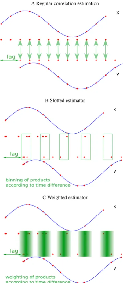
Fig. 1: Principles of correlation function estimation: (A) shows the classical estimator, where the correlationρˆxy(k)is given by a mean over products of zero-mean observations a lagkapart. (B) For irregularly sampled time series, the slot-ted estimator computesρˆxy(k)as the mean over all products in bins whose centers are a lagkapart. (C) Non-rectangular correlation uses the weighted mean over all available prod-ucts with the weight maxima a lagkapart.
the persistence time of autoregressive processes of order 1 (AR(1)) (Mudelsee, 2002).
2 Methods
Assuming that two time seriesxtandytwere observed from stationary stochastic processes at unit time intervals, their sample CCFρˆ(k)gives an estimate of the strength of a pos-sible linear association between the processes behind the ob-servations at each possible lag numberk. It is defined as
ˆ
ρxy(k) = ˆρxy(k∆τ) = ˆγxy(k)/ˆσxσˆy (1)
= 1
ˆ
σxσˆy(N−k) N−k
X
t=1
(xt−¯x)(yt+k−y¯). (2)
Here,ˆγxy(k)is the sample cross-covariance at lagk,N is the number of observations,ˆσx,σˆy the sample standard deviations of the processes andx¯,y¯are the estimated mean values of the time series (Chatfield, 2004). The spacing of the CCF lags,∆τ, equals – in this standard definition – that of the time seriesxtandyt,∆τ=tx,yi −t
x,y i+1.
The discrete Fourier transform of the sample CCF is the sample cross spectral density function or cross spectrum and vice versa. The power spectrum can thus be estimated in two ways, either by computing the discrete Fourier trans-forms of the input time series and multiplying them after complex-conjugating one of them, or by estimating the CCF and Fourier transforming it (cf. (Chatfield, 2004) for more details). We denote all estimators in the definitions in their respective sections byρˆ, for the sake of simplicity.
2.1 The resampling approach for irregular time series
In the case of irregularly sampled time series, the classical definition, as illustrated in Fig. 1A, can not be readily ap-plied. An irregularly spaced time series is a pair (tx,x) of tuples of common lengthNx, wheretx
1< tx2<···< txNxare
the time points andxi is the value at timetxi. For simplic-ity we have transformed the time variable to get a normal-ized mean increment of 1 by dividing by the mean sam-pling period: tx
i =t orig
i /∆tx and we will use this notation in the following. The differences between observation times
∆tx
i =txi−txi−1are then not any more constant and the mean
of their distribution is the mean sampling time∆tx. When we consider irregularly sampled time series(tx,x),(ty,y)of second-order stationary processes with zero mean, these have to be resampled onto a common regular time grid (tx,y) with constant time incrementstx,y(n)−tx,y(n−1) = ∆t
xfor all
n= 1,2,...Nx,y. The grid spacing we will use is the larger of the mean sampling intervals of the time series.
We restrict ourselves in this analysis to the linear inter-polation technique, as the effects of other standard routines are not much different in their variance reduction towards the high-frequency end of the spectrum (Schulz and Stattegger, 1997). A resampling method which does not result in a re-duction in variance is thenearest neighbor technique, where the function is approximated at the desired grid points by the value of the observation closest in time. This leads to a Fig. 1. Principles of correlation function estimation: (A) shows the
classical estimator, where the correlationρˆxy(k)is given by a mean over products of zero-mean observations a lagkapart. (B) For irreg-ularly sampled time series, the slotted estimator computesρˆxy(k)as the mean over all products in bins whose centers are a lagkapart. (C) Non-rectangular correlation uses the weighted mean over all available products with the weight maxima a lagkapart.
consider irregularly sampled time series (tx,x), (ty,y) of second-order stationary processes with zero mean, these have to be resampled onto a common regular time grid (tx,y) with constant time incrementstx,y(n)−tx,y(n−1)=1tx for all
We restrict ourselves in this analysis to the linear inter-polation technique, as the effects of other standard routines are not much different in their variance reduction towards the high-frequency end of the spectrum (Schulz and Stattegger, 1997). A resampling method which does not result in a re-duction in variance is the nearest neighbor technique, where the function is approximated at the desired grid points by the value of the observation closest in time. This leads to a shifting bias (Broersen, 2009) which, in the presence of large gaps in the data, can be rather large. We therefore do not em-ploy this scheme. After resampling, the standard FFT-based routines can be employed.
2.2 Lomb-Scargle approach
The Lomb-Scargle approach to the spectral estimation of ir-regularly sampled data can be understood as a least squares fitting of sinusoids to data (Scargle, 1981). The Lomb-Scargle Fourier transform (LSFT)
LSFTx(ω)=F0(ω)
Nx
X
i=1
(Axi cosωtˆix+iBxi sinωtˆix),(3)
uses the explicit observation timestˆx
i =tix−τx(ω)shifted by
the constant (complex) phase shift
τx(ω)= 1
2ωtan
−1 X
i
sin2ωtix/X
i
cos2ωtix
!
, (4)
to ensure time invariance of the LSFT (Schulz and Stattegger, 1997). The coefficientF0
F0(ω)= 1
√
2exp(
−i ωt1x−τx(ω)) (5)
allows for a time shift in the alignment of the two time series in bivariate spectral analysis. The amplitudesAandB are defined as
A(ω)= X
i
cos2ωtˆix
!−1/2
, B(ω)= X
i
sin2ωtˆix
!−1/2
. (6) In the univariate case, the well-known Lomb-Scargle peri-odogram is then given by
ˆ
Px(ω)=LSFTx(ω)LSFT∗x(ω) (7)
The (bivariate) cross spectrum can be estimated as
ˆ
Pxy(ω)=LSFTx(ω)LSFT∗y(ω) (8)
which can be inverted, using the Fourier transform (Scargle, 1989), to get the cross correlation coefficient estimate
ˆ
ρxy(k)=F−1[ ˆPxy(ω)]. (9)
The squared absolute value of the LSFT gives the widely known and used LS periodogram (Schulz and Stattegger,
1997). The choice of the frequenciesωis described in Scar-gle (1989) and we adopt the recommended values for the fundamental frequencyω0=ωmin= π(N
xy−1)
(tmax−tmin)Nxy and
maxi-mum frequencyωmax=1t2πxy. In the bivariate case we define
the observation timestmin andtmaxas the lower and upper bounds of the overlapping part of both time series xt and
yt, otherwise, in the univariate case, minimum and
maxi-mum observation time are used. 1txy=max(1tx,1ty)is
the common sampling rate we define in the bivariate case. The number of frequencies Nf=ofac·Nxy determines the spacing of the frequency vector. According to Hocke and K¨ampfer (2009) there is no principal limit, the oversampling factor ofac>1 is regarded as a smoothing factor, although the number of independent frequencies is constant. We use ofac=2, unless otherwise stated.
A thorough introduction to bivariate Lomb-Scargle spec-tral estimation was given by Schulz and Stattegger (1997). The use of the technique for correlation function estimation, however, has not yet been explored, though it was already proposed in Scargle (1989).
2.3 Correlation slotting
The sample correlation function ρˆxy(k) at a lag k is
cal-culated by averaging over the lagged products of the standardized observations. For irregular time series the inter-sampling times vary, and without resampling Eq. (1) cannot be applied. An alternative is the slotting or Edelson and Krolik technique (Edelson and Krolik, 1988; Mayo, 1993). Its key idea is to calculate the cross-products of all available, standardized, observations and discretize them into bins according to their sampling time differences as can be seen in Fig. 1b. The technique was developed in fluid me-chanics and applied in astrophysics. ρ(k1τ )ˆ at the lagk1τ is then defined as
ˆ
ρ(k·1τ )= PNx
i=1 PNy
j=1xiyjbk(tjy−tix)
PN i=1
PN
j=1bk(tjy−tix)
(10)
and the kernelbk(tjy−tix)selects the products whose time lag
is not further than half the bin width fromk1τ: bk(ti−tj)=
1 for||(tj−ti)| −k|<12
0 otherwise. (11)
Note that the observations have to be standardized to zero mean and unit variance before the analysis. We set the lag bin width1τ to be equal to1txy, and since we divide the ob-servation times by this mean sampling interval, we can omit it in the formulae above, for easier readability (cf. Sect. 2.1). We do not choose this width arbitrarily but rather in the con-text of the desired time resolution of the CCF, more on this in Sect. 2.4.
Fig. 2. Kernel-based estimators effectively “use” observations whose inter-sampling time difference is close to the lag for which linear correlation is estimated. Slotting (the rectangular kernel) chooses observations within an interval, Gaussian and sinc kernel weigh the products smoothly according to the difference between observation interval and desired lag. Kernels were scaled to the standard choice for width parameterh(cf. Table 1, Fig. 3).
due to which we will not use this method in the following, but rather apply related, non-rectangular kernels. It also does not always provide positive semidefinite covariance matrix estimates, a problem which can be overcome by “fourier fil-tering”. We discuss this further in Sect. 2.5.
2.4 Non-rectangular kernels
In analogy to the slotting approach, and taking it further, weighted averaging of the observations can be performed us-ing symmetric, smooth density functions that tend to zero for time differences much larger or smaller than the desired lag k(Hall et al., 1994). The similarity is illustrated in Fig. 1c. These requirements are for example met by the sinc kernel (Stoica and Sandgren, 2006) but also the Gaussian kernel (cf. Table 1) as can be seen in Fig. 2. Instead of binning the observations into discrete sets, the weights prevent a sudden cutoff in the time domain.
There is no theoretical definition of the effective width of the weight functions. We decide to scale them to a kernel width of the mean sampling rate for two reasons. (i) This choice ensures that – for non-rectangular kernels – observa-tions at (near-)regular times are rated higher than those that are further away, but are still included in cases where little information is available. (ii) In a trade-off between the loss of resolution and control of estimator variance, the desired resolution of the correlation function also plays a role, as a kernel width choice larger than the lag spacing would result in mixing information for adjacent lags. The width param-eters for the kernels and their relation to the mean sampling rate were confirmed as empirical optima in case of irregular
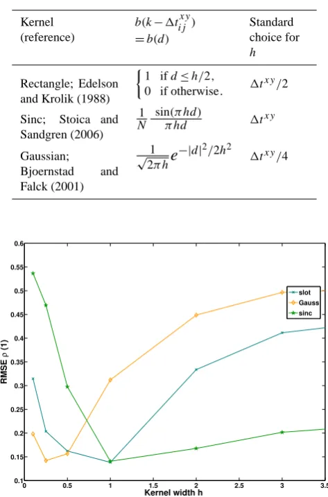
Table 1. Kernelsb(d)used in this paper. d denotes the distance between the inter-observation time1tijxyand k1τ,k denotes the
k-th lag. The standard width parameterhis chosen to result in a main lobe width of1txy, the mean sampling interval or common sampling period in the bivariate case.
Kernel (reference)
b(k−1tijxy)
=b(d)
Standard choice for
h
Rectangle; Edelson and Krolik (1988)
1 ifd≤h/2,
0 if otherwise. 1t xy/2
Sinc; Stoica and Sandgren (2006)
1
N
sin(π hd)
π hd 1txy
Gaussian;
Bjoernstad and Falck (2001)
1
√
2π h
e
−|d|2/2h2 1txy/4
0 0.5 1 1.5 2 2.5 3 3.5
0.1 0.15 0.2 0.25 0.3 0.35 0.4 0.45 0.5 0.55 0.6
Kernel width h
RMSE
ρ
(1)
slot Gauss sinc
Fig. 3. Influence of varying kernel widthhon the RMSE ofρ(1), using the kernel estimators (cf. Table 1, Fig. 2). 100 Realizations of sinusoids with random phase in colored noise (30 %) were sampled using0−distributed sampling intervals (sk = 2.85). (cf. Sect. 3.3).
time series (cf. Fig. 3). Other parameter choices might, how-ever, also be sensible, depending on the nature of the time series and the statistic to be estimated.
2.5 Positive semidefiniteness of the estimated function
In connection with the slotting-based covariance estimation, the issue with the possible lack of positive semidefiniteness of the correlation estimates has been discussed in Broersen (2002), Harteveld et al. (2005) and Stoica and Sandgren (2006). By Bochner’s theorem, positive semidefiniteness of the correlation function is necessary and sufficient to ensure non-negativity of the Fourier transform estimate ofρ(t ). Aˆ
Z Z ˆ
ρ(l−t )w(t )w(l)dt dl≥0 (12) for all integrable functionsw, and only if this holds trueρ(k)ˆ
is a possible correlation function. For discrete, short, and regularly sampled time series, using Eq. (10) and a simple, integrable function forw, we can find this condition violated for all kernel methods. This problem can, amongst others, be solved by a technique called “Fourier filtering”, which involves Fourier-transforming the correlation function esti-mate, setting any negative power estimates to zero and apply-ing an inverse FFT afterwards to obtain a positive semidef-inite correlation function estimate (Babu and Stoica, 2009; Hall et al., 1994). Another routine could involve using the absolute value of the power spectrum, instead of setting neg-ative estimates to zero. Also, positive semidefinite matrices have non-negative eigenvalues, which is another means to test this property, and the same modifications as for the power spectra could be applied here. It should be kept in mind, how-ever, that, due to numerical problems, even the “unbiased” 1/(N−1)correlation estimator can result in negative power estimates. When the positive semidefiniteness of the correla-tion matrix is essential, Fourier filtering should be performed and/or the eigenvalues of the matrix should be checked. 2.6 Quality of performance measures
Our aim is to evaluate which of the approaches listed above yields the best results for the estimation of ACFs and CCFs for geophysical time series. The performance of the esti-mators can be evaluated with respect to the “true” expected functions. This can of course only be done for modeled or synthetic time series where we can calculate ACFs and CCFs exactly.
To evaluate the different estimators we calculate the root mean square error (RMSE) of the estimatorθˆfor a statistic
θ.θcan be e.g. the cross correlation function at lagk,ρxy(k).
The RMSE is given by RMSE(θ )ˆ =
q
E[(θˆ−θ )2] = q
var(θ )ˆ +bias(θ )ˆ 2 (13)
and incorporates both variance and bias of the estimator, i.e. its variability and its systematic deviation from the true value. To estimate the RMSE we generate a large number of time series of a given signal type and sampling scheme and com-pute the “target statistic”θˆfor each. The deviation between
the mean of these many estimates and the ‘true’ function is the approximate bias of the estimator, together with the vari-ance around this mean we can estimate the RMSE.
To evaluate the contribution of the sampling irregularity to the estimation error, we perform the analysis for differ-ent sampling schemes, first for regular sampling and then for more and more irregular sampling. This we do by drawing inter-sampling-time intervals from the Gamma-distribution
and concatenating them into a time line for which we then generate a corresponding signal. Given the shape parame-terαand the scale parameterβ, the meanµof the 0(α,β)-distribution is given byµ=αβ, the variance byσ2=αβ2 and the skewness by sk=2/√α. For low skewness (in our case the lowest value was 0.1) the distribution is close to nor-mal (cf. Fig. 7b). Since the higher order moments depend only on the shape parameterα, we can vary the scale param-eterβ in a way to keep the mean constant while increasing skewness and variance. We will only give the skewness pa-rameter in the following, as the variance σ2=(2β/sk)2=
(2µ/(skα))2is uniquely determined in our parameter con-figuration. A distribution with a skewness of 2.85 (Fig. 7b) results in a time series with large gaps, as large values be-come more likely in more and more skewed sampling inter-val distributions.
3 Comparison for synthetic records
To assess the adaptability and suitability of the different es-timators, we perform a number of tests on artificially gen-erated discrete signals for which we know the “true” ACFs and/or CCFs of the underlying processes. For each signal type we first estimate the RMSE in the case of regular sam-pling. Then we create time series with0-distributed inter-observation times with increasing skewness. Since the time vectors are artificial, they do not need to have an actual unit, but we assume that time is measured in years.
3.1 Sinusoids with random phase
Using techniques that are not (yet) fully established, our first concern is to make sure that the results for the standard, reg-ularly sampled case are consistent with those from the stan-dard estimators. Therefore we sample a simple signal, a su-perposition of three sinusoids:
x(t )= 3 X
i=1
sin(ωit+2i,n) (14)
withωi=2Tiπ, Ti=(18,21,41)yr at a regular rate of 1/4
years. The phase variable2i,n is randomly drawn from a
uniform distribution on(0,2π ), making this a sample from a stationary stochastic process. The true ACF is then a super-position of cosine functionsρxx=1/2P3i=1 cos(ωi),
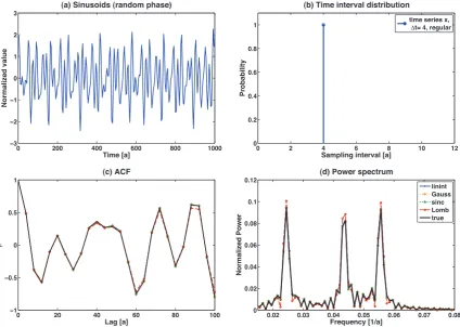
irre-spective of the relative phases of the signal components. The length of the simulated time series is 1000 yr and we evaluate the function for 200 lags. Sample time series, mean ACF and power spectral density (PSD) of the mean ACF are depicted in Fig. 4. The kernel estimators, the LS periodogram as well as the “classical” method perform comparably well with a RMSE below 2 % (see Fig. 5, left columns) in the regularly sampled case.
0 200 400 600 800 1000 −3
−2 −1 0 1 2 3
(a) Sinusoids (random phase)
Time [a]
N
o
rm
a
li
ze
d
v
a
lu
e
0 2 4 6 8 10 12 0
0.2 0.4 0.6 0.8 1
Sampling interval [a]
Pr
o
b
a
b
il
ity
(b) Time interval distribution
time series x,
Δt= 4, regular
0 20 40 60 80 100 −1
−0.5 0 0.5 1
(c) ACF
Lag [a]
ρ
0.02 0.03 0.04 0.05 0.06 0.07 0.08 0
0.02 0.04 0.06 0.08 0.1 0.12
Frequency [1/a]
N
o
rm
a
li
ze
d
Po
w
e
r
(d) Power spectrum
linint Gauss sinc Lomb true
Fig. 4. Autocorrelation analysis of synthetic signals: for a regularly sampled combination of sinusoids (cf. Eq. 14) we give a sample time series (a), the sampling interval probability density (b), the expected correlation function (c) and the corresponding power spectrum (d) determined from 100 realizations of sinusoid time series with random phase arguments. Legends for each row are given in the right panels. All estimators perform equally well.
Fig. 5. Mean RMSE for the ACF estimation (lags 1–3) using lin-ear interpolation, Gaussian or sinc kernel or the inversion of the Lomb-Scargle periodogram of noise-free sinusoids given for reg-ular, gamma-distributed and mildly irregular (skewness sk = 0.1) resp. very irregular (sk = 2.85) sampling. Errorbars give the stan-dard deviation of the estimate, calculated using 1000 bootstrap iter-ations.
skewness (as described in Sect. 2.6). For skewness sk = 0.1 the RMSEs are only slightly higher (Fig. 5, middle columns), but for a skewness sk = 2.85 the RMSE is as high as 40 % for interpolation and 35 % for the LS method. The estimated RMSE for the Gaussian kernel method, is rather small com-pared to that, with an approximate 12 %, lower than that of the sinc kernel method (23.5 %). We have increased the skewness in steps of 0.25 from sk = 0.1 to sk = 2.85 and note that the RMSE of the ACF seems to be increasing almost lin-early for all the methods. For the LS estimate it jumps in the beginning, from 5 % to≈20 %, and continues to increase at a rate of 9 % per unit skewness, with the breakpoint occur-ring at a skewness of 0.35. The RMSE of the interpolation followed by the FFT-based estimator (denoted “linint” in the figure legends) increases at a faster overall rate than all the other methods (6.5 % per unit skewness). The Gaussian ker-nel method has the lowest RMSE at high skewness and the lowest increase with respect to the estimate for regular sam-pling.
0 200 400 600 800 1000 −2
−1.5 −1 −0.5 0 0.5 1 1.5 2 2.5
(a) Sinusoids (random phase)
Time [a]
N
o
rm
a
li
ze
d
v
a
lu
e
0 2 4 6 8 10 12 0
0.5 1 1.5 2 2.5 3 3.5 4 4.5
x 10−3
Sampling interval [a]
Pr
o
b
a
b
il
ity
(b) Time interval distribution
time series x, Δt= 4 and Γ(0.5, 8)−distributed
0 20 40 60 80 100 −1
−0.5 0 0.5 1
(c) ACF
Lag [a]
ρ
0.02 0.03 0.04 0.05 0.06 0.07 0.08 0
0.02 0.04 0.06 0.08 0.1 0.12 0.14
Frequency [1/a]
N
o
rm
a
li
ze
d
Po
w
e
r
(d) Power spectrum
linint Gauss sinc Lomb true
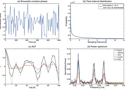
Fig. 6. Autocorrelation analysis of synthetic signals: for an irregularly sampled combination of sinusoids (cf. Eq. 14) we give a sample time series (a), the sampling interval probability density (b), the expected correlation function (c) and the corresponding power spectrum (d) determined from 100 realizations of sinusoid time series with random phase arguments. Legends for each row are given in the right panels. High sampling irregularity leads to a variance reduction in the ACF for LS and interpolation.
input signal frequencyω=2π/18 (c.f. Figs. 4d and 6d). We find, that with increasing skewness, the RMSE of this peak increases from around 3 % to 10 % for interpolation and the LS correlation function estimate, while for sinc and Gaussian kernel it goes from<1 % to approximately 2 %. Estimating the bias of this peak, we observe that the comparatively high RMSE for interpolation and LS method corresponds to a neg-ative bias increasing linearly from 5 % to>50 % with respect to the expected peak power at the high-frequency component. In contrast to that, the bias is nearly constant for the kernel methods, the slight increase in RMSE must therefore be due to an increase in variance. This lack of power in the high frequency component of the estimated spectrum is accompa-nied by a positive bias for the lowest frequency component ω=2π/100 (results not shown).
3.2 Autoregressive processes
To understand the quantitative and qualitative effect of the different estimation techniques on the short-term correlative properties (e.g. the persistence time, the lag at which the ACF has dropped to 1t /e), we use AR(1) processes generated
at high time resolution and then re-sample the observations onto the desired irregular sampling times. We perform the same simulations as before, first evaluating for regular sam-pling and then, for gamma-distributed samsam-pling inter-vals, where we subsequently increase the skewness of the interval distribution. The driving process is given by X(ti)=φX(ti−1)+ξi=e−1t /τX(ti−1)+ξi (15)
and for bivariate correlation analysis we sample a second process driven by the first at lag`:
Y (ti)=αX(ti−`)+εi. (16)
0 200 400 600 800 1000 −4
−3 −2 −1 0 1 2 3 4
(a) Coupled AR1
Time [a]
Normalized value
0 0.5 1 1.5 2 2.5 3
0 0.5 1 1.5 2 2.5 3 3.5 4
x 10−3
Sampling interval [a]
Probability
(b) Time interval distribution
time series x, ∆t= 1
and Γ(4e+02,0.003)−distributed
time series y, ∆t= 1
and Γ(0.5, 2)−distributed
0 5 10
0 0.2 0.4 0.6 0.8 1
(c) ACF x
Lag [a]
ρ
0 5 10
(d) ACF y
Lag [a]
−100 −5 0 5 10
0.1 0.2 0.3 0.4 0.5
(e) CCF
Lag [a]
ρxy
linint Gauss sinc Lomb theoretical
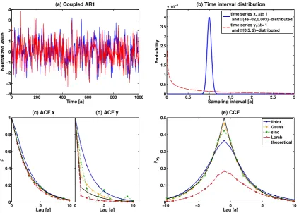
Fig. 7. Cross correlation analysis for two irregularly sampled signals (cf. Eqs. 15, 16) from different sampling schemes: Sample time series (a) and sampling time interval histograms (b), the mean ACFs out of 100 realizations (c) and the mean estimated CCF (d). Legends for each row are given in the right panels. A positive bias in interpolation ACF estimates and a negative bias in the interpolation and LS CCF estimates is observable for increased sampling irregularity.
In the estimation of the AR(1) coefficientφ, the RMSE for interpolation increases from 2 % to 17 % and the error for the sinc-kernel increases from 6 % to 13.5 %. The LS technique results in the largest increase for high skewness with a RMSE of 52 %. The Gaussian kernel method remains more accurate with an increase from 2 % to 8.5 %.
The coupling strengthαis the true value of the CCF at the coupling lag`. A typical application in the geoscience context is the estimation of the degree of similarity for time series from different sources, with different sampling prop-erties. Analyzing two time series of inter-sampling time dis-tribution skewnesses skx=0.1 sky=2.85, we find that the
CCF estimation at lag`= −1 has a negative bias for all tech-niques. The bias of the LS technique is strongly negative, underestimating the true correlation by more than 65 %. Lin-ear interpolation results in a 30 % lower estimated coupling strength, the sinc kernel method in 15 % and the Gaussian kernel estimate is negatively biased by 8 % with respect to the “true” coupling strength of 0.5 (Fig. 7e).
Looking at the performance under the increasing sampling time distribution skewness of time series yt (keeping skx
constant at 0.1), we find that the RMSE of the estimatedα
Fig. 9. RMSE for the CCF estimation (at the lag of coupling) us-ing linear interpolation, Gaussian or sinc kernel or the inversion of the LS Periodogram of time series from coupled AR(1) processes (cf. Eqs. 15, 16) – given for regular and two gamma-distributed sam-plings with mildly irregular (skewness skxand sky=0.1) and very irregular (skewness skx=0.1, sky=2.85) inter-observation-times. Errorbars give the standard deviation of the estimate, calculated us-ing 1000 bootstrap iterations.
increases for all methods, but least for the Gaussian kernel (Fig. 9).
3.3 Sinusoids with random phase in colored noise
For irregular time series, the effect of interpolation on the ACF estimation of noise-free sinusoids is that it seems to suppress high-frequency variability. For red-noise signals we find that it, similarly, leads to an overestimation of autocor-relation. To generate more “realistic” signals, we synthesize the above-mentioned sinusoidal signals (Eq. 14) with varying amounts of additive red (AR) noise:
x(t )=1−s
3
X
i
sin(ωit+2i,n)+sζi. (17)
The sinusoidal components vary with the frequenciesωi=
2π
Ti,Ti= [18,21,41]years. The time vectortis concatenated
into a time line from random variables drawn from a gamma-distribution withµ=4 and sk = 0.1. The phase variable2i,n
is, for each realizationn, randomly drawn from a uniform distribution on(0,2π ). This makes the time series samples from stationary stochastic processes.ζirepresents a red noise
process (cf. Eq. 15) whose variances we vary in the range
[0,1]. The persistence time τ is, for this intercomparison, fixed atτ=4 (corresponding toφ≈0.78). Since we adjust the overall variance of the process to equal unity, the signal-to-noise ratio varies in proportion withs.
The “true” ACF is then given by ρ(k)=(1−s)/3X
i
cos( ωi|k|)+s·exp(−|k|/τ ) . (18)
0 0.1 0.2 0.3 0.4 0.5 0.6 0.7 0.8 0.9 1
0.05 0.1 0.15 0.2 0.25 0.3
Mean RMSE
ρ
(1)
fraction of total variance due to noise
linint Gauss sinc Lomb
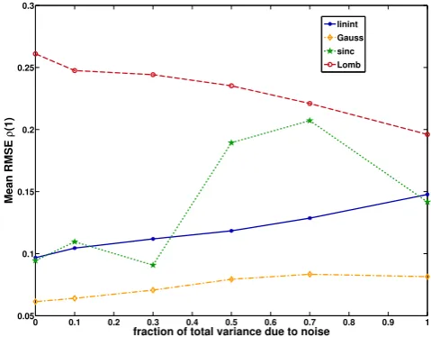
Fig. 10. Effect of the Signal-to-Noise ratio on the RMSE of the ACF for skewed (sk = 2) inter-observation times. The share of the noise variance in the overall process variance increases from left to right (cf. Eq. 17).
Varyingsand using irregular time series (sk = 2) we find that the mean RMSE ofρˆx(1)estimated for the Gaussian
ker-nel method increases slightly from 5 % for sinusoidal signals (s=0, cf. Fig. 10), to 7 % for pure red noise (s=1). At the same time, the RMSE for the interpolation-based routine rises from 10 % to 15 %, that for the LS-technique decreases from 27 % to 19 %. The sinc kernel performs similar to the interpolation routine for sinusoidal signals with up to 30 % of noise, but has a higher RMSE for noise-dominated signals. For irregular time series with low inter-sampling-time distri-bution skewness (sk = 0.1) we find that the RMSE is maximal for medium signal-to-noise ratios, i.e. it is lower for purely deterministic and purely random time series than for the mix-ture of both (results not shown). For mostly deterministic time series,s60.5, the LS technique has then the highest RMSE, while sinc and Gaussian kernel-based methods give more accurate results. For dominant red noises>0.5, the LS technique gives good results with low RMSE, where at the same time the performance of the sinc kernel deterio-rates. The interpolation-based FFT-routine is not the best choice for irregular time series, irrespective of the signal-to-noise ratios of the processes generating the time series. The increased RMSE for interpolation observable for the ACF es-timates is due to a positive bias forρx(1). The RMSE of the
3.4 Summary of the synthetic tests
In all tests we performed in this section, we find that linear interpolation comes with two systematic effects. Firstly, it has a positive bias for ACF estimation and secondly, it has a negative bias in CCF estimation. Both effects become more severe with increasing sampling time distribution skewness. The LS technique performed well for the ACF estimation of slightly irregular autocorrelated time series but not for sinu-soids. We find the opposite pattern for the sinc kernel: its RMSEs are low in the application to sinusoidal data – but high for the ACF of autocorrelated noise processes. The Gaussian kernel estimates are consistent and have the, or close to the, lowest RMSEs in all tests. Therefore we recom-mend the use of the Gaussian kernel-based estimator instead of – or in addition to – the standard interpolation routine for irregular time series with positive inter-sampling time distri-bution skewness, and especially in the presence of observa-tion gaps.
4 Comparison for paleo data
We will now apply the Gaussian kernel estimator and in-terpolation followed by the standard FFT-routine to paleo records from the Asian Monsoon domain, to evaluate pos-sible differences between the CCF/ACF estimates of these datasets, depending on the analysis technique.
The Asian monsoon system (cf. Fig. 11) affects a large share of today’s world population. Zhang et al. (2008) find its strength in the past 1800 yr to be correlated with agricul-tural and culagricul-tural prosperity, its weakening with periods of unrest and instability. It can be divided into the Indian and the East Asian monsoon subsystems (ISM and EASM), that transport moisture from different sources. Oxygen isotope ratios (δ18O) from cave records have been used to study the Holocene variability of monsoonal precipitation over China and India. While most of them show a millennial-scale trend, believed to be linked with the decreasing solar irra-diation through the Holocene (Maher, 2008; Wang et al., 2005), sources for variability on shorter time scales are de-bated (Berkelhammer et al., 2010). In an inter-comparison of four published, acclaimed records of monsoonal precipi-tation from four different geographical locations we want to investigate the spatial and temporal consistency of linear de-pendencies among these time series. Cross-correlation anal-ysis of monsoon records could give clues to the interrelation-ships between the different monsoon branches and their de-velopment with time. Autocorrelation analysis can, amongst other methods, give insights into the persistence inherent to the time series and is believed to increase before certain dy-namical transitions (Scheffer et al., 2009). Persistence time (cf. Eq. 15) is a characteristic parameter for the time scales on which these climate processes operate.
70°E
80°E 90°E 100°E 110°E 120°E 130°E 10°N
20°N 30°N
Dandak
Wanxiang Heshang
Dongge
Bay of Bengal
Pacific South
China Sea
Fig. 11. Map showing the location of the paleo records and the main wind directions of the Indian and East-Asian summer monsoon sys-tems. Presently there are three major inflow corridors into Southern China, through the Bay of Bengal and over Indo-China, through the South China Sea and from the south east (Liu et al., 2008; Clemens et al., 2010).
For the late Holocene time span of 387–1100 BP, we estimate cross correlation and persistence time of four speleothem δ18O records (cf. Fig. 11), reconstructed from Dongge cave in southern China (Wang et al., 2005), Hes-hang cave in central China (Hu et al., 2008), Wanxiang cave in north-central China (Zhang et al., 2008) and from Dan-dak cave in southern India (Berkelhammer et al., 2010). The sample locations lie in different branches of the Asian mon-soon and therefore enable us to assess spatial variability of the monsoon system. The data sets have quite different inter-sampling time distributions, with rather high time resolution (0.5a–3.9a) and considerable time uncertainties. The details of the overlapping part of the records, which we will use, are given in table 2. For all four records, δ18O variations are interpreted as mainly dominated by precipitation amount changes, thus reflecting summer monsoon strength (Wang et al., 2005; Hu et al., 2008; Zhang et al., 2008; Berkelham-mer et al., 2010).
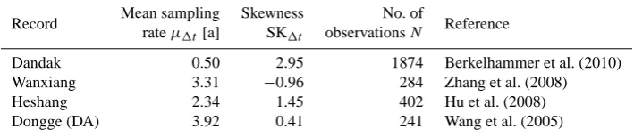
Table 2. Mean sampling intervals,variances and skewnesses of the inter-sampling time distributions and number of observations in the overlapping section of the used paleo proxy records (625 AD–1563 AD).
Record Mean sampling Skewness No. of Reference
rateµ1t[a] SK1t observationsN
Dandak 0.50 2.95 1874 Berkelhammer et al. (2010)
Wanxiang 3.31 −0.96 284 Zhang et al. (2008)
Heshang 2.34 1.45 402 Hu et al. (2008)
Dongge (DA) 3.92 0.41 241 Wang et al. (2005)
4.1 Results from ACF analysis
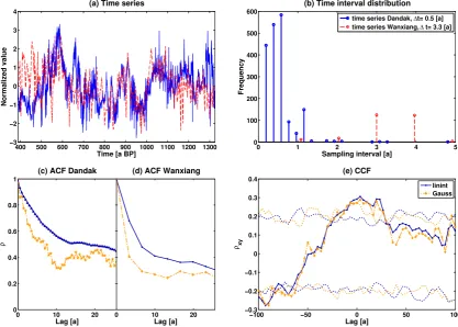
First we look at the individual ACFs (e.g. Fig. 12c and d) and find that the Gaussian estimate shows a much stronger initial decline than that resulting from interpolation. To in-vestigate whether this more pronounced decline, this lower persistence timeτ (cf. Eq. 15), is due to a negative bias of the kernel method or to a positive bias of the interpolation we perform the additional least squares analysis (LSq). The esti-mator, implemented similar to that in Mudelsee (2002), fits a simplified Ohrnstein-Uhlenbeck process, a continuous-time AR(1) analog, to the time series. Its estimates are robust with respect to variations in sampling rates, irregularity and per-sistence time and show a small, but constant, bias (−10 %) and variance. We compare four results: from interpolation, followed by ACF estimation involving the FFT; from inter-polation, followed by the LSq estimation; from the Gaussian kernel ACF estimate and from LSq analysis of the original record (cf. Fig. 13). We find a pronounced overestimation, up to a factor of two, when interpolation is involved. This is ir-respective of whetherτ was estimated via ACF or the LSq fit. The Gaussian kernel estimate is generally lower than that of LSq analysis, but differs by not much, except in the estimate for the Heshang cave record where it is 50 % lower. We could relate this to the differences in the respective sampling time distributions: The Heshang sampling time distribution shows high skewness and a large mean sampling period, both com-bining into a source of estimation error. Neither high skew-ness (Dandak) nor a lower sampling rate (Dongge) alone lead to such a deviation between the LSq and Gaussian kernel es-timates, which is in agreement with the results from Sect. 3.
It follows from this, that interpolation causes a strongly positive bias on persistence and the kernel-based estimate is slightly negatively biased. Thus, if in an analysis the two es-timates coincide we could assume the result to be unbiased. On the other hand, we should exercise caution when the re-sults from different methods disagree. Persistence times give a measure of memory in processes and are thus important to characterize time scales on which climate processes operate. As we see in this section, interpolation leads to a strong over-estimation of persistence for irregular time series, with a bias changing also in relation to the skewness of the observation time distribution. Caution should therefore be exercised and
additional methods employed when performing autocorrela-tion analysis of irregular time series.
4.2 Results from cross correlation analysis
Next, pairwise cross correlation functions were calculated for all four records. Only two combinations resulted in signifi-cant correlation at zero lag (Fig. 14a). The correlation co-efficient of 0.29 (−0.17,0.21) for interpolation resp. 0.295 (−0.19,0.27) for the Gaussian kernel at lag zero between the Wanxiang and Dandak records is significant to the 95 % level in the two-sided test for zero correlation under the null hy-pothesis of the time series being sampled from autocorrelated red noise processes. In the brackets we give the estimated critical values of the test that were determined using AR(1) processes (with persistence times based on the LSq estimate) on the original time axis of the records.
The late Holocene section (387–1325 BP) of the record from Wanxiang cave correlates also significantly with that from Heshang cave with a lag zero correlation coeffi-cient of 0.28 (−0.2, 0.23) based on interpolation and 0.28 (−0.2,0.19) from the kernel estimator. We find that the high-frequency variability of the estimated correlation function is more pronounced in the kernel estimate. However, the over-all shapes of the functions agree well.
400 500 600 700 800 900 1000 1100 1200 1300 −3
−2 −1 0 1 2 3 4
(a) Time series
Time [a BP]
Normalized value
0 1 2 3 4 5
0 100 200 300 400 500 600
Sampling interval [a]
Frequency
(b) Time interval distribution
time series Dandak, ∆t= 0.5 [a] time series Wanxiang, ∆ t= 3.3 [a]
0 10 20
0 0.2 0.4 0.6 0.8 1
(c) ACF Dandak
Lag [a]
ρ
0 10 20
(d) ACF Wanxiang
Lag [a]
−100 −50 0 50 100
−0.3 −0.2 −0.1 0 0.1 0.2 0.3 0.4
Lag [a]
(e) CCF
ρxy
linint Gauss
Fig. 12. Exemplary cross correlation analysis ofδ18O records from Dandak and Wanxiang caves: Standardized time series (a), the sampling interval distributions (b), the estimated ACFs (c, d) and the corresponding CCF with the dashed lines representing the estimated 95 % critical values of a two-sided test for the null hypothesis of time series being sampled from a red noise process (e). Legends for each row are given in the right panels.
Fig. 13. Persistence times of theδ18O records estimated using lin-ear interpolation ACF estimate, Gaussian kernel ACF estimate and the least squares fitting of AR(1) processes (denoted by LSq) on interpolated and original record.
The Asian summer monsoon is a large-scale atmospheric circulation phenomenon. During northern hemisphere cold phases, less energy available for its generation might have
led to a weakening of the monsoon. In contrast, warm phases should have led to a strong circulation which results in an in-creased influence of the ISM on Chinese precipitation. This should be observable in an increased correlation between In-dian and Chinese rainfall variation and, at the same time, an increased correlation between theδ18O records.
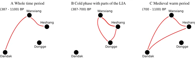
We therefore analyze two time slices (389 BP–700 BP and 700 BP–1100 BP) of the records separately. After signifi-cance testing – and considering lags of 0 to 30 yr absolute value –, we find a contrasting picture: while the North-ern Chinese records correlate with the Indian Dandak record during the warm phase (MWP), this correlation is insignif-icant in the colder phase (towards the LIA) that followed (cf. Fig. 14c). On the other hand, while the southern Chinese Dongge record correlates with the more northern records from Heshang and Wanxiang caves during the LIA, this cor-relation is not significant during the MWP.
A Whole time period
Dandak
Dongge Heshang Wanxiang (387 - 1100) BP
B Cold phase with parts of the LIA
Dandak
Dongge Heshang Wanxiang (387-700) BP
C Medieval warm period
Dandak
Dongge Heshang Wanxiang (700 - 1100) BP
Fig. 14: Results from pairwise cross correlation analysis for all records: Red links indicate significant positive cross correlation at or close to zero lag for the respective records. While in the warm phase of the MWP the Northern Chinese records correlate with the Indian Dandak record and not with the southernmost Dongge cave record (C), this is reversed in the cold phase after the MWP. The Chinese records then correlate amongst each other, but not with the Indian Dandak record (B).
varying sampling irregularity. Compared to this, interpola-tion leads to an overestimainterpola-tion of this persistence time by a factor of two. This difference is especially unnerving as the frequency of observations recorded through paleo archives varies in dependence on climatic parameters (e.g. lower ac-cumulation rates through less precipitation). A change in the inter-observation time distribution could then lead to an arti-ficial change in the estimated persistence.
In the cross correlation analysis of the paleo records, the kernel-based lag-zero cross correlation functions are consis-tent for interpolation and cross correlation. We believe that this is due to the short time scales on which the interac-tions of the monsoon systems are recorded, as the advan-tages of the kernel-based method are not as pronounced for records with high persistence. The kernel-based cross corre-lation functions show more high-frequency variability which could be investigated through cross spectral analysis. We do not attempt to characterize it here, since this is outside the scope of this paper. The bias effects from interpolation could cause problems in the evaluation of phenomena emerg-ing on time scales close to the actual mean samplemerg-ing rate. This is where the kernel methods show significant advantages and especially the Gaussian kernel correlation method can provide high-resolution, robust estimates of time-dependent cross correlation coefficients.
In our cross correlation analysis of four Asian monsoon records in the time interval of 387BP–1100BP, we have found significant evidence that the Indian summer mon-soon circulation influenced Chinese rainfall variability dur-ing the northern hemispheric MWP, as then theδ18O record
from Dandak cave in India correlates with the central China records from Wanxiang and Heshang caves. During the colder phase after the MWP and into the LIA, significant cross correlation coefficients are found amongst the Chinese records, indicating a spatially more homogeneous moisture source. At the same time these records do not correlate with
the Indian record during the LIA cold phase, pointing to less ISM impact on Chinese precipitation.
To summarize, we have shown that in correlation estima-tion of irregularly sampled time series, cauestima-tion should be ex-ercised when these records have an inter-observation time distribution that is strongly skewed. In the CCF estimation we found a strongly negative bias for the standard approach with interpolation for processes with little persistence. The advantages of the kernel-based estimators are higher for cou-pling on short time scales, compared to the samcou-pling rate. This is especially interesting for the investigation of proxy data with low resolution. Our results indicate that the bias properties of the Gaussian kernel and the interpolation tech-niques have different signs in ACF estimation, indicating when sampling irregularity causes problems in the analysis.
Acknowledgements
This research was financially supported by the the German Federal Ministry of Education and Research (BMBF project PROGRESS, 03IS2191B), the German Science Foundation (DFG graduate school 1364) and by the Leibniz associa-tion (project ECONS). The authors would like to thank Jef-frey D. Scargle and one anonymous referee as well as Se-bastian Breitenbach for their valuable and insightful advice. Software to analyze irregularly sampled time series using the methods in this paper can be found on www.tocsy.pik-potsdam.de
References
Babu, P. and Stoica, P.: Spectral analysis of nonuniformly sampled data - a review, Digit. Signal Process., 20, 359–378, doi:10.1016/ j.dsp.2009.06.019, 2009.
Fig. 14. Results from pairwise cross correlation analysis for all records: Red links indicate significant positive cross correlation at or close to zero lag for the respective records. While in the warm phase of the MWP the Northern Chinese records correlate with the Indian Dandak record and not with the southernmost Dongge cave record (B), this is reversed in the cold phase after the MWP. The Chinese records then correlate amongst each other, but not with the Indian Dandak record (C).
“isotopic zone” where both monsoonal branches are influ-ential. However, Dongge cave lies closer to the southern zone that is, at present, dominated by monsoonal precipi-tation from the south east (South China Sea) but not from the south-west (ISM). Recent investigations show, that even within southern China, moisture sources and their isotopic signature, differ orthogonally to these “isotopic zones” (Liu et al., 2008), pointing at a stronger influence of the South East monsoon in direction of Dongge cave. We conclude that during warm phases our results are consistent with these isotopic zones, since the records from central China corre-late with the Indian Dandak record. In the cold phases, the atmospheric circulation might have been different, emphasiz-ing the south east moisture source for allover China, evident through a correlation between the Dongge cave record and the more northern Chinese records and, since we observe no significant correlation with the Dandak record, less ISM im-pact.
Interpolation and kernel-based estimation give similar re-sults. The CCF estimates at and around lag zero were not – or not significantly – lower for interpolation where a significant correlation was detected. We believe that this is due to the long time scales on which these correlations are recorded, as the advantages of the kernel-based method are larger for low persistence (cf. Sect. 3).
5 Conclusions
Comparing different methods for analyzing correlations from irregularly sampled time series, we have found that the kernel-based method is robust and has a comparable – and often even lower – RMSE and bias than the traditionally em-ployed schemes using interpolation in the application to syn-thetic records, for regular and irregular sampling.
For the interpolation and FFT-based routine we find a four to seven times increase in RMSE, predominantly caused by an increase in the absolute value of the bias. This bias is
positive for ACF estimation but negative for CCF quantifica-tion and its magnitude scales linearly with sampling irregu-larity.
In all synthetic test cases we studied the Gaussian kernel was close to or was the estimator with the lowest RMSE. Its performance was slightly inferior to that of the sinc ker-nel for sinusoidal time series but significantly better for red noise ACF and CCF estimation, especially in the application to records with disparate sampling rates.
We find that the sinc-kernel performs well for ACF estima-tion of sinusoidal signals. It shows, however, alternating bias patterns in the ACF for red noise time series, resulting in a high RMSE comparable to the FFT-based result. This might be due to the shape of the kernel with its positive and nega-tive weights, thus emphasizing regular, deterministically re-current structures that are not present in stochastic processes. Another reason for the mixed performance could be cutoff effects, since the kernel effectively presents a rectangular fil-ter in the frequency domain.
The performance of the Lomb-Scargle periodogram-based routine showed advantages over interpolation for low skew-ness time sampling. For very irregular time series, in ACF as in CCF tests, we found a strong sampling effect resulting in a large bias.
In all tests we performed on synthetic data, we have found that linear interpolation comes with two systematic effects: It shows a positive bias for ACF estimation, and it has a negative bias in CCF estimation, emphasizing low-frequency variability at the cost of high-frequency components. Both effects become more severe with increasing sampling time distribution skewness and lower persistence in the processes from which we generate the time series. The Gaussian ker-nel estimates are consistent with those from interpolation for regular sampling and have the, or close to the, lowest RMSEs in all tests.
squares persistence time estimator, which is, fitting an AR(1) process to the observations, has a constant and low bias for varying sampling irregularity. Compared to this, interpola-tion leads to an overestimainterpola-tion of this persistence time by a factor of two. This difference is especially unnerving as the frequency of observations recorded through paleo archives varies in dependence on climatic parameters (e.g. lower ac-cumulation rates through less precipitation). A change in the inter-observation time distribution could then lead to an arti-ficial change in the estimated persistence.
In the cross correlation analysis of the paleo records, the kernel-based lag-zero cross correlation functions are consis-tent for interpolation and cross correlation. We believe that this is due to the short time scales on which the interac-tions of the monsoon systems are recorded, as the advan-tages of the kernel-based method are not as pronounced for records with high persistence. The kernel-based cross corre-lation functions show more high-frequency variability which could be investigated through cross spectral analysis. We do not attempt to characterize it here, since this is outside the scope of this paper. The bias effects from interpolation could cause problems in the evaluation of phenomena emerg-ing on time scales close to the actual mean samplemerg-ing rate. This is where the kernel methods show significant advantages and especially the Gaussian kernel correlation method can provide high-resolution, robust estimates of time-dependent cross correlation coefficients.
In our cross correlation analysis of four Asian monsoon records in the time interval of 387 BP–1100 BP, we have found significant evidence that the Indian summer mon-soon circulation influenced Chinese rainfall variability dur-ing the northern hemispheric MWP, as then theδ18O record from Dandak cave in India correlates with the central China records from Wanxiang and Heshang caves. During the colder phase after the MWP and into the LIA, significant cross correlation coefficients are found amongst the Chinese records, indicating a spatially more homogeneous moisture source. At the same time these records do not correlate with the Indian record during the LIA cold phase, pointing to less ISM impact on Chinese precipitation.
To summarize, we have shown that in correlation estima-tion of irregularly sampled time series, cauestima-tion should be ex-ercised when these records have an inter-observation time distribution that is strongly skewed. In the CCF estimation we found a strongly negative bias for the standard approach with interpolation for processes with little persistence. The advantages of the kernel-based estimators are higher for cou-pling on short time scales, compared to the samcou-pling rate. This is especially interesting for the investigation of proxy data with low resolution. Our results indicate that the bias properties of the Gaussian kernel and the interpolation tech-niques have different signs in ACF estimation, indicating when sampling irregularity causes problems in the analysis.
Acknowledgements. This research was financially supported by the
the German Federal Ministry of Education and Research (BMBF project PROGRESS, 03IS2191B), the German Science Foundation (DFG graduate school 1364) and by the Leibniz association (project ECONS). The authors would like to thank Jeffrey D. Scargle and one anonymous referee as well as Sebastian Breitenbach for their valuable and insightful advice. Software to analyze irregularly sampled time series using the methods in this paper can be found on www.tocsy.pik-potsdam.de.
Edited by: S. Barbosa
Reviewed by: J. Scargle and another anonymous referee
References
Babu, P. and Stoica, P.: Spectral analysis of nonuniformly sam-pled data - a review, Digit. Signal Process., 20, 359–378, doi:10.1016/j.dsp.2009.06.019, 2009.
Benedict, L., Nobach, H., and Tropea, C.: Benchmark tests for the estimation of power spectra from LDA signals, in: Proc. 9th Int. Symp. on Applications of Laser Technology to Fluid Me-chanics, p. 32.6, Lisbon, Portugal, 1998.
Benedict, L., Nobach, H., and Tropea, C.: Estimation of turbulent velocity spectra from laser Doppler data, Meas. Sci. Technol., 11, 1089, doi:10.1088/0957-0233/11/8/301, 2000.
Berkelhammer, M., Sinha, A., Mudelsee, M., Cheng, H., Edwards, R. L., and Cannariato, K.: Persistent multidecadal power of the Indian Summer Monsoon, Earth Planet. Sc. Lett., 290, 166–172, doi:10.1016/j.epsl.2009.12.017, 2010.
Bjoernstad, O. N. and Falck, W.: Nonparametric spatial covariance functions: Estimation and testing, Environ. Ecol. Stat., 8, 53–70, doi:10.1023/A:1009601932481, 2001.
B¨ottcher, M. and Dermer, C. D.: Timing Signatures of the Internal-Shock Model for Blazars, The Astrophysical Journal, 711, 445, doi:10.1088/0004-637X/711/1/445, 2010.
Broersen, P. M.: Autoregressive spectral estimation by application of the Burg algorithm to irregularly sampled data, IEEE T. In-strum. Meas., 51, 1289–1294, doi:10.1109/TIM.2002.808031, 2002.
Broersen, P. M.: Five Separate Bias Contributions in Time Series Models for Equidistantly Resampled Irregular Data, IEEE T. In-strum. Meas., 58, 1370, doi:10.1109/TIM.2009.2012928, 2009. Broersen, P. M., de Waele, S., and de Waele, S.: The Accuracy of
Time Series Analysis for Laser-Doppler Velocimetry, in: Pro-ceedings of the 10th International Symposium on Applications of Laser Techniques to Fluid Dynamics, Lisbon, Portugal, 2000. Chatfield, C.: The analysis of time series: an introduction, Texts in
statistical science, CRC Press, Florida, US, 6th Edn., 2004. Clemens, S. C., Prell, W. L., and Sun, Y.: Orbital-scale timing and
mechanisms driving Late Pleistocene Indo-Asian summer mon-soons: Reinterpreting cave speleothemδ18O, Paleoceanography, 25, 4207–4223, doi:10.1029/2010PA001926, 2010.
Edelson, R. and Krolik, J.: The discrete correlation function – A new method for analyzing unevenly sampled variability data, As-trophys. J., 333, 646–659, doi:10.1086/166773, 1988.