www.ocean-sci.net/13/427/2017/ doi:10.5194/os-13-427-2017
© Author(s) 2017. CC Attribution 3.0 License.
Measuring pH variability using an experimental sensor on an
underwater glider
Michael P. Hemming1,2, Jan Kaiser1, Karen J. Heywood1, Dorothee C.E. Bakker1, Jacqueline Boutin2, Kiminori Shitashima3, Gareth Lee1, Oliver Legge1, and Reiner Onken4
1Centre for Ocean and Atmospheric Sciences, School of Environmental Sciences, University of East Anglia, Norwich
Research Park, Norwich NR4 7TJ, UK
2Laboratoire d’Océanographie et du Climat, 4 Place Jussieu, 75005 Paris, France
3Tokyo University of Marine Science and Technology, 4-5-7 Konan, Minato, Tokyo 108-0075, Japan 4Helmholtz-Zentrum Geesthacht, Max-Planck-Straße 1, 21502 Geesthacht, Germany
Correspondence to:Michael P. Hemming ([email protected]) Received: 29 September 2016 – Discussion started: 11 October 2016 Revised: 1 April 2017 – Accepted: 28 April 2017 – Published: 24 May 2017
Abstract.Autonomous underwater gliders offer the capabil-ity of measuring oceanic parameters continuously at high res-olution in both vertical and horizontal planes, with timescales that can extend to many months. An experimental ion-sensitive field-effect transistor (ISFET) sensor measuring pH on the total scale was attached to a glider during the REP14-MED experiment in June 2014 in the Sardinian Sea in the northwestern Mediterranean. During the deployment, pH was sampled at depths of up to 1000 m along an 80 km transect over a period of 12 days. Water samples were col-lected from a nearby ship and analysed for dissolved inor-ganic carbon concentration and total alkalinity to derive the pH for validating the ISFET sensor measurements. The ver-tical resolution of the pH sensor was good (1 to 2 m), but sta-bility was poor and the sensor drifted in a non-monotonous fashion. In order to remove the sensor drift, a depth-constant time-varying offset was applied throughout the water col-umn for each dive, reducing the spread of the data by ap-proximately two-thirds. Furthermore, the ISFET sensor re-quired temperature- and pressure-based corrections, which were achieved using linear regression. Correcting for this de-creased the apparent sensor pH variability by a further 13 to 31 %. Sunlight caused an apparent sensor pH decrease of up to 0.1 in surface waters around local noon, highlight-ing the importance of shieldhighlight-ing the sensor from light in fu-ture deployments. The corrected pH from the ISFET sensor is presented along with potential temperature, salinity, po-tential density anomalies (σθ), and dissolved oxygen
con-centrations (c(O2)) measured by the glider, providing
in-sights into the physical and biogeochemical variability in the Sardinian Sea. The pH maxima were identified close to the depth of the summer chlorophyll maximum, where high c(O2) values were also found. Longitudinal pH variations at
depth (σθ>28.8 kg m−3) highlighted the variability of water
masses in the Sardinian Sea. Higher pH was observed where salinity was>38.65, and lower pH was found where salin-ity ranged between 38.3 and 38.65. The higher pH was as-sociated with saltier Levantine Intermediate Water, and it is possible that the lower pH was related to the remineralisation of organic matter. Furthermore, shoaling isopycnals closer to shore coinciding with low pH andc(O2), high salinity,
alka-linity, dissolved inorganic carbon concentrations, and chloro-phyll fluorescence waters may be indicative of upwelling.
1 Introduction
It is estimated that one-third of the anthropogenic carbon dioxide emitted between 2004 to 2013 was absorbed by the oceans (Le Quéré et al., 2015). Normally unreactive in the atmosphere, carbon dioxide dissolved in seawater (CO2(aq))
takes part in a number of chemical reactions. In particular, carbonic acid (H2CO3) forms as a result of (CO2(aq))
428 M. P. Hemming et al.: Measuring pH using an experimental sensor in the Sardinian Sea
(c(DIC), with “c” representing a concentration) with HCO−3 accounting for 90 % of c(DIC). During the dissociation of carbonate species, hydrogen ions (H+) are released. The pH
is calculated as the negative decadal logarithm of the activity (commonly referred to as a concentration) of these H+ions. Thus the pH in the ocean is directly related to the activity of H+ions in the water (Zeebe and Wolf-Gladrow, 2001).
The pH varies on timescales spanning less than 1 day (Hofmann et al., 2011) to many years (Rhein et al., 2013). Since before the industrial revolution (year 1760), the global surface ocean pH has fallen from 8.21 to 8.10 (correspond-ing to a 30 % increase in H+ ion activity) as a result of the atmospheric CO2mole fraction increasing by more than
100 µmol mol−1(Doney et al., 2009; Fabry et al., 2008). Fu-ture projections of anthropogenic carbon dioxide emissions suggest that ocean uptake of CO2 will continue for many
decades, thus contributing to long-term ocean acidification (Rhein et al., 2013). This may have a significant effect on ma-rine organisms, such as calcifying phytoplankton (e.g. coc-colithophores) and corals (e.g. scleractinian), dependent on the solubility state of calcium carbonate (Doney et al., 2009). Since 1989, it has been possible to measure pH to an accuracy of 10−3 using a spectrophotometric approach (Byrne and Breland, 1989). Although there have been some advances in adapting this approach to measure pH au-tonomously in situ (Martz et al., 2003; Aßmann et al., 2011), spectrophotometry is largely used for shipboard measure-ments, as it requires the use of indicator dye and a means to measure spectrophotometric blanks, which is challenging outside of a laboratory (Martz et al., 2010).
A limited number of hydrographic surveys have been un-dertaken, and stations offering long-term time series of pH are available (Rhein et al., 2013). However, there is a drive to improve spatial and temporal data coverage via autonomous means, similar to what was experienced for temperature and salinity with Argo floats 16 years ago (Roemmich et al., 2003). There is demand to develop a reliable autonomous sensor with a precision and accuracy of 10−3that is afford-able to the scientific community (Johnson et al., 2016).
The Mediterranean Sea comprises just 0.8 % of the global oceanic surface, but it is regarded as an important sink for anthropogenic carbon due to its physical and biogeochem-ical characteristics (Álvarez et al., 2014). Between 1995 and 2012, surface c(DIC) increased by 3 µmol kg−1a−1 in the northwest Mediterranean Sea, which is consistent with a rise in temperature of 0.06◦C a−1 and a decrease in pH of 0.003 a−1 (Yao et al., 2016). In contrast, the pH in
the neighbouring North Atlantic Ocean decreased by just 0.0017 a−1associated with an increase inc(DIC) of around 1.4 µmol kg−1a−1 and a temperature rise of 0.01◦C a−1 (Bates et al., 2012). The greater potential of the Mediter-ranean Sea to store anthropogenic carbon can be explained by its higher alkalinity, warmer temperatures, and thus lower Revelle factor (Álvarez et al., 2014; Touratier and Goyet,
2011) when compared with other oceans, such as the North Atlantic.
The pH in the Mediterranean Sea is typically higher than most other oceanic regions (Álvarez et al., 2014). The pH on the total scale normalised to 25◦C (pHT ,25) collected
by ship between 1998 and 1999 within the northwestern Mediterranean Sea varied between 7.92 and 8.04 at the sur-face and between 7.9 and 7.93 at depths greater than 100 m (Copin-Montégut and Bégovic, 2002). When considering the Mediterranean Sea as a whole, pHT ,25 obtained by ship in
April 2011 varied between 7.98 and 8.02 at the surface and between 7.88 and 7.96 at greater depths (Álvarez et al., 2014). The peak-to-peak amplitude of the annual pH cycle in the northwest Mediterranean Sea is typically 0.1 with max-ima and minmax-ima in spring and summer, respectively (Yao et al., 2016).
Measurements of pH with higher temporal resolution, such as those measured by in situ sensors, can vary greatly depending on their location and depth. Hofmann et al. (2011) presented the results of 15 deployments using SeaFET pH sensors (Sea-Bird Scientific) close to the surface at a number of locations worldwide. They found that pH could vary by as much as 1.1 in extreme environments, such as those obtained close to volcanic CO2vents off the coast of Italy, or as little
as 0.02 in open ocean areas, such as in the temperate east-ern Pacific Ocean, over a time period of 30 days. Hofmann et al. (2011) were able to capture diel cycles in pH, with the most consistent variations found in coral reef locations. The pH was at a maximum in the early evening and at a mini-mum in the morning with amplitudes between 0.1 and 0.25; this is similar in range to other studies based in subtropical estuaries (Yates et al., 2007).
Autonomous underwater gliders offer the possibility to ob-serve the oceanic system with a greater level of detail on both temporal and spatial scales when compared with ship measurements (Eriksen et al., 2001). A low consumption of battery power and a great degree of manoeuvrability enable such vehicles to cover large areas and profile depths of up to 1000 m during missions that can last from weeks to months. They are suitable platforms for a range of sensors, measur-ing both physical and biogeochemical parameters (Piterbarg et al., 2014; Queste et al., 2012).
Figure 1.The locations of the 93 dives undertaken by the Seaglider (red markers), the eight ship CTD casts in which water samples were obtained (white markers), and meteorological buoy M1 (yellow marker) within the REP14-MED observational domain off the coast of Sardinia, Italy between 11 and 23 June 2014. GEBCO 1 min resolution bathymetry data (metres) were used (http://www.bodc.ac.uk/projects/ international/gebco/), and surface circulation patterns were adapted from figures presented by Millot (1999).
The initial pH results and validation, the method of further correcting pH, and an artefactual light-induced effect are de-scribed in Sect. 3.2.2. Corrected pH measurements are anal-ysed alongside other collected parameters in Sect. 3.2.3, and the conclusions are presented in Sect. 4.
2 Methodology
2.1 REP14-MED sea trial
This trial took place between 6 and 25 June 2014 in the northwest Mediterranean Sea off the coast of Sardinia, Italy (Fig. 1). This was part of the Environmental Knowledge and Operational Effectiveness (EKOE) research programme led by the North Atlantic Treaty Organisation (NATO) Centre for Maritime Research and Experimentation (CMRE) based in La Spezia, Italy. This was the fifth Recognised Environ-mental Picture (REP) trial, which was jointly conducted by two research vessels: the NRVAllianceand the RVPlanet.
Eleven gliders with varying pressure tolerances were de-ployed during the trial, each making repeated west–east tran-sects separated by roughly 0.13◦ of latitude from one an-other within the REP14-MED observational domain. One of these gliders was operated by the University of East Anglia (UEA): an iRobot Seaglider model 1KA (SN 537) with an ogive fairing. All gliders were deployed to meet the objec-tives of the trial, such as to improve ocean forecasting tech-niques (e.g. model validation and evaluation of forecasting skill), conduct a cost–benefit analysis of autonomous gliders, analyse mesoscale and sub-mesoscale features, and test new glider payloads. The latter objective was perhaps the most relevant to the deployment of the UEA glider. A more in-depth overview of the REP14-MED trial, its objectives, and the collected observational data is described by Onken et al. (2016).
The UEA glider completed a total of 126 dives between 11 and 23 June 2014. The first 24 dives did not record pH and the last 9 dives were very shallow, leaving 93 usable dives. Suc-cessive dives were approximately 2 to 4 km apart, descending to depths of up to 1000 m.
2.2 Glider sensors
Conductivity, pressure, and in situ temperature measure-ments were obtained by the glider using a Sea-Bird Scien-tific glider payload CTD sensor (Bellevue, WA, USA; Fig. 2). These measurements were then used to obtain potential tem-perature (θ) and practical salinity.
Dissolved oxygen concentrations (c(O2), where “c” refers
to a concentration) were measured using an Aanderaa 4330 oxygen optode sensor (Aanderaa Data Instruments, Bergen, Norway) positioned towards the rear of the glider fairing (Fig. 2). The method of calibratingc(O2) closely followed
that described by Binetti (2016), using the oxygen sensor en-gineering parameters TCPhase and CalPhase, which will be summarised here. The first step involved correctingc(O2) to
account for the response time (τ) of the sensor, as the dif-fusion of oxygen across the silicon foil of the sensor is not an instantaneous process. Each oxygen sensor has a differ-ent τ, which depends on the structure, thickness, age, and usage of the foil (McNeil and D’Asaro, 2014), as well as the external environmental conditions such as temperature. An average τ of 17 s was obtained using the method out-lined by Binetti (2016). After correcting the TCPhase forτ, glider TCPhase profiles were matched in time and space with pseudo-CalPhase profiles back-calculated from the measure-ments ofc(O2) obtained by the ship Sea-Bird Scientific SBE
430 M. P. Hemming et al.: Measuring pH using an experimental sensor in the Sardinian Sea
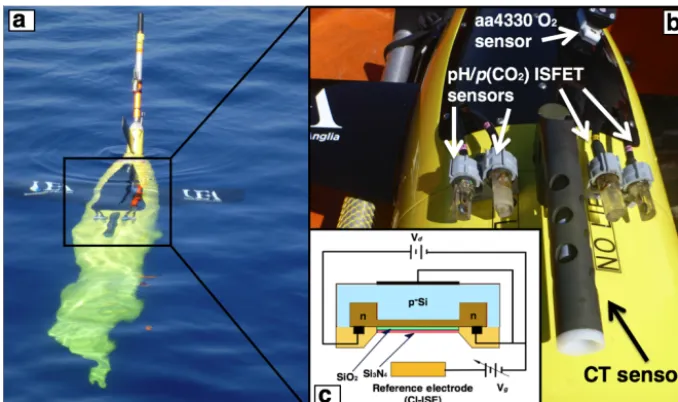
Figure 2. (a)Seaglider SN 537 during the deployment:(b)a close-up of the sensors and(c)a schematic diagram of the ISFET sensor adapted from Shitashima (2010).
used to correct the glider CalPhase, which is required for calibratingc(O2) measurements. A comparison between the
ship c(O2) measurements and the calibrated glider c(O2)
measurements is made in Sect. 3.2.1.
Glider variables have been processed using an open-source MATLAB-based toolbox (https://bitbucket.org/ bastienqueste/uea-seaglider-toolbox/) in order to correct for differing timestamp allocations, sensor lags (Garau et al., 2011; Bittig et al., 2014), and to tune the hydrodynamical flight model (Frajka-Williams et al., 2011). Outliers outside of a specified range (e.g. 6 standard deviations) were flagged and not used for analysis, and glider profiles were smoothed using a lowess low-pass filter with a span of 5 data points (<4 m range), which implements a local regression using weighted linear least squares and a first-order polynomial linear model. Individual profiles were inspected afterwards to ensure that potentially correct data points were not removed.
The ISFET pH sensor used in this study (Fig. 2) was cus-tom built by a working group led by Kiminori Shitashima at the Tokyo University of Marine Science and Technology (previously the University of Kyushu), and it is not com-mercially available. The ISFET unit was housed in acrylic resin material. The ISFET unit and the reference chlorine ion-selective electrode (Cl-ISE) were moulded with epoxy resin in the custom-built housing. The ISFET pH unit was stand-alone, meaning that the sensor was not integrated into any of the onboard glider electronics. The power source of the sensor was 10.5 V supplied by three 3.5 V Li-ion batter-ies.
The glider also carried another ISFET pH sensor that was integrated into the glider electronics (Fig. 2) and twop(CO2)
sensors (Shitashima, 2010), one stand-alone and one
inte-grated. The data retrieved from the integrated pH sensor and thep(CO2) sensors could not be used due to quality issues.
We think the regular on/off cycling of power to the integrated dual pH–p(CO2) sensor between sampling did not allow it to
function properly. In future, we would suggest the addition of backup batteries to supply power to the sensor between sam-pling. The cause of the problem with the stand-alonep(CO2)
unit is unclear.
To measure pH, the activity of H+ions is determined us-ing the interface potential between the Cl-ISE and the semi-conducting ion-sensing transistor coated with silicon diox-ide (SiO2) and silicon nitride (Si3N4). The ISFET pH
sen-sor was previously found to have a response time of a few seconds with an accuracy of 0.005 pH and suitable tempera-ture and pressure sensitivities (Shitashima et al., 2002, 2013; Shitashima, 2010). Before deploying the sensor, the ISFET and Cl-ISE were conditioned (as recommended by Bresna-han et al., 2014 and Takeshita et al., 2014) in a bucket of lo-cal sea surface water with a salinity of 38.05. However, due to time constraints, conditioning took place over just 1 hour rather than weeks as specified by Bresnahan et al. (2014) and Takeshita et al. (2014). During the deployment, pH measure-ments were obtained vertically every 1 to 2 m.
buffer solutions takes into account the effect of changing air temperature, ranging between 30.5 and 33.3◦C during
pre-calibration and between 27.5 and 28◦C during
post-calibration. A linear fit using the raw output measured from these buffer solutions was used to convert the raw counts to pH (Shitashima et al., 2002). A drift was observed between the pH of these buffer solutions before and after the deploy-ment, which was corrected for. As the ISFET sensor was pre-viously described as having a pressure-resistant performance and good temperature characteristics for oceanographic use (Shitashima et al., 2002; Shitashima, 2010), no compensa-tions for temperature and pressure were performed on the ISFET measurements at this stage. The ISFET pH sensor has a salinity sensitivity of∂pH/ ∂S=0.011, which was taken into account. The effect of biofouling on the ISFET pH mea-surements, as well as on all other glider meamea-surements, was ruled out after a post-deployment inspection of the sensors indicated no problems.
2.3 Ship-based measurements
As the in situ ISFET pH sensor was under trial, some form of validation of the results was required. In total, 124 water sam-ples were collected from Niskin bottles sampled at 12 depths (down to 1000 m) using a CTD rosette platform at eight lo-cations (eight casts, numbered 24–51) close to the path of the glider (Fig. 1). Water samples were collected between 05:19 local time (LT, UTC+2) on 9 June and 16:58 LT on 11 June. The glider ISFET pH sensor started operating at 16:36 LT on 11 June. Overall, the measurements obtained by the glider and the CTD overlapped better in space than in time (Fig. 3). When collecting carbon samples, water was drawn into 250 mL borosilicate glass bottles from Niskin bottles on the CTD rosette using tygon tubing. Bottles were rinsed twice before filling and were overflowed for 20 s, allowing the bottle volume to be flushed twice. Each sample was poi-soned with 50 µL of saturated mercuric chloride and then sealed using greased stoppers, secured with elastic bands, and stored in the dark (Dickson et al., 2007). The total al-kalinity (AT) and thec(DIC) of each water sample was
mea-sured in the laboratory using a Marianda Versatile INstru-ment for the Determination of Titration Alkalinity (VIN-DTA 3C; www.marianda.com). The c(DIC) was measured by coulometry (Johnson et al., 1985) following standard op-erating procedure SOP 2, and AT was measured by
poten-tiometric titration (Mintrop et al., 2000) following SOP 3b, both described by Dickson et al. (2007). During the analyti-cal process, 21 bottles of certified reference material (CRM; batch 107) supplied by the Scripps Institution of Oceanog-raphy (San Diego, CA, USA) were run through the ment to keep track of stability and to calibrate the instru-ment. For each day in the lab, one CRM was used before and after the samples were processed. A total of 19 concurrent replicate-depth water samples were collected with around 2 to 3 replicates per CTD cast. Calculating the mean
stan-dard deviation of these replicate samples enabled a measure-ment of the instrumeasure-ment precision. The mean standard devia-tions of thec(DIC) andATreplicates were 1.7 µmol kg−1and
1.4 µmol kg−1, respectively. This corresponds to a pH uncer-tainty of 0.003 forc(DIC) andAT, resulting in a combined
uncertainty of 0.009.
OnceATandc(DIC) were known, pH could be derived
us-ing the CO2SYS programme (Van Heuven et al., 2011). This calculation has an estimated pH probable error of around 0.006 due to uncertainty in the dissociation constantspK1
andpK2(Millero, 1995). Temperature and salinity were
ob-tained from the Sea-Bird CTD sensor on the ship rosette sampler, and the seawater equilibrium constants presented by Mehrbach et al. (1973) were used as refitted by Dickson and Millero (1987), which has been recommended by previ-ous studies (e.g. the CARINA data synthesis project) for the Mediterranean Sea (Álvarez et al., 2014; Key et al., 2010). The sulfate constant described by Dickson (1990) and the pa-rameterisation of total borate presented by Uppström (1974) were used. More information on the equilibrium constants used in CO2SYS and other available carbonate system pack-ages is described by Orr et al. (2015). The pH derived from the water samples collected by ship and the glider-retrieved ISFET pH are both on the total pH scale (as described by Dickson, 1984) at in situ temperature and will from now on be referred to as pHsand pHg, respectively.
Standard deviation ranges will from this point be listed when referring to variability in measurements, such as pHs
and pHg. To obtain these standard deviation ranges, data
points for a given variable were sorted into 10 m depth bins down to a maximum depth of 1000 m. The standard deviation was then calculated for each bin.
3 Results and discussion 3.1 Ship-based data
Measurements obtained by the ship CTD package provide an overview of the temporal and spatial variability for the time at which the water samples used to derive pHswere
432 M. P. Hemming et al.: Measuring pH using an experimental sensor in the Sardinian Sea
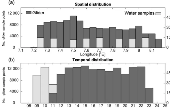
Figure 3.Histograms showing the(a)spatial and(b)temporal distribution of samples collected by the glider (dark grey) and by CTD water bottle sampling (light grey). Theyaxis on the left is for the sum of the glider samples, whilst theyaxis on the right is for the sum of the water samples.
east of 7.5◦E, which is likely to be Levantine Intermediate
Water (LIW) identified in the western Mediterranean Sea by a salinity range of 38.45 to 38.65 andθ between 13.07 and 13.88◦C (Rivaro et al., 2010), typically found at depths be-tween 200 and 800 m close to the shelf slope (Millot, 1999). The c(O2) maxima were found at depths between 20 and
90 m. The Mediterranean Sea on the whole is considered to be oligotrophic (Álvarez et al., 2014). However, a deep chlorophyll maximum (DCM) is common at these depths when waters are thermally stratified (Estrada, 1996). There is a build-up of actively growing biomass with greater cell pig-ment content as a result of photoacclimation due to increased concentrations of nitrate, phosphate, and silicate, as well as sufficient levels of light at these depths (Estrada, 1996). It is likely that this highc(O2) was related to the DCM, further
ev-idenced by the high chlorophyll fluorescence layer observed at 60 to 100 m of depth, particularly in the east.
The objective of deriving pHs using AT andc(DIC) was
to make a comparison with the pHgmeasured by the ISFET
sensor. The c(DIC) and AT were greatest at depths below
250 m with lower values seen closer to the surface (Fig. 5a– b), which is typical of the northwest Mediterranean Sea (Copin-Montégut and Bégovic, 2002; Álvarez et al., 2014). The higher values of AT and c(DIC) at depth and in the
east support the notion that this is LIW, as this water mass has previously been identified as having an AT of around
2590 µmol kg−1 and a c(DIC) of roughly 2330 µmol kg−1 (Álvarez et al., 2014), coinciding with the warmer saltier waters. The mean c(DIC) and AT (averages over eight
casts) have standard deviations of 6.1 to 11.9 and 5.9 to
10.6 µmol kg−1, respectively, for the top 150 m of the water column and 1.7 to 3.9 µmol kg−1 and 3.7 to 7.6 µmol kg−1 for deeper waters. The pHshad a maximum of 8.14 between
50 and 70 m of depth (Fig. 5c). The mean pHs values have
standard deviations of 0.004 to 0.011 within the top 150 m and 0.006 to 0.017 deeper than this. A proportion of these standard deviations can be explained by the instrumental er-ror associated with the analysis ofc(DIC) andATdiscussed
in Sect. 2.3.
3.2 Glider data
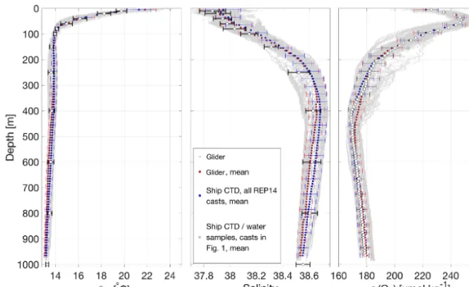
3.2.1 Temperature, salinity, and oxygen validation Since the sensors were calibrated before deployment, it was expected that the measurements from the glider would match those from the CTD because any discrepancies between datasets would indicate possible instrumental or methodolog-ical issues with the glider measurements. The mean profiles ofθ, salinity, andc(O2) collected by the glider and by ship
(Fig. 6) agreed well. The values obtained by both ship and glider were mostly within 1 standard deviation of one an-other. The meanθand salinity retrieved during the eight ship pHscasts differed from the binned mean calculated using all
available REP14-MED ship casts at depths between 100 and 500 m. However, this is likely related to temporal or spatial variability as meanθ and salinity were within the range of all available glider measurements. Furthermore, differences of roughly 0.1◦C, 0.02, and 1.5 µmol kg−1 can be seen for θ, salinity, andc(O2), respectively, between the binned mean
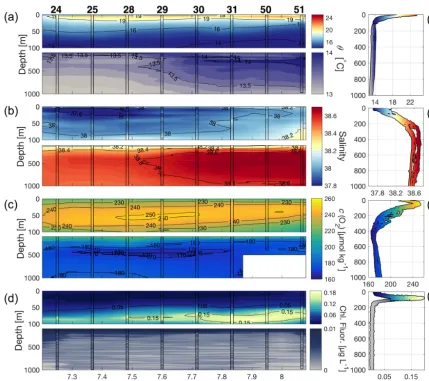
Figure 4.Transects of optimally interpolated(a)potential temperature (θ),(b)salinity,(c)dissolved oxygen concentrations (c(O2)), and(d) chlorophyll fluorescence, along with their depth profiles(e–h)obtained by ship. These parameters were sorted into 0.1◦longitude×5 m bins, and the radius of influence used for optimal interpolation was 0.2◦longitude×20 m. The data retrieved during the eight CTD casts (displayed in Fig. 1) used for optimal interpolation are superimposed on the interpolated fields.
of glider measurements at depths greater than 500 m. These differences inθ, salinity, andc(O2) are related to the
differ-ent spatial distribution of the two datasets, as the glider mea-sured predominantly at 40◦N where deep, cooler, and fresher waters were observed in the west (Fig. 4a–b) that are uncom-mon in other areas of the observational domain (Knoll et al., 2015b).
3.2.2 ISFET pH validation
The mean pHg and pHs agreed best between 60 and 250 m
(Fig. 7), although pHg variability was a lot higher than for
pHs. Larger differences between these profiles can be seen
above and below this depth range, with a pHg0.1 higher at
the surface and roughly 0.07 lower between 950 and 1000 m when compared with pHs. The pHs maximum at
approxi-mately 50 to 70 m of depth was not apparent in the pHg
pro-file, with the highest pHgseen at the surface. The standard
deviations for pHg were large, ranging between 0.044 and
0.114 in the top 150 m of the water column and between 0.027 and 0.053 at other points in the water column. Com-paring all pHgdive profiles obtained during the mission
sug-gests a great degree of temporal and spatial variability, with pH ranging from 8.02 to 8.28 at the surface and between 7.97 and 8.13 at 800 m of depth.
A diel cycle in pHg anomalies (calculated by
subtract-ing the all-time mean from the hourly means within a given depth interval) was found predominantly at depths shal-lower than 20 m (Fig. 8b). Lower pH was found between 09:00 and 18:00 LT, decreasing by>0.1 between 12:00 and 14:00 LT. Contrastingly, potential temperature, salinity, and c(O2) anomalies (calculated in the same way as pHg
434 M. P. Hemming et al.: Measuring pH using an experimental sensor in the Sardinian Sea
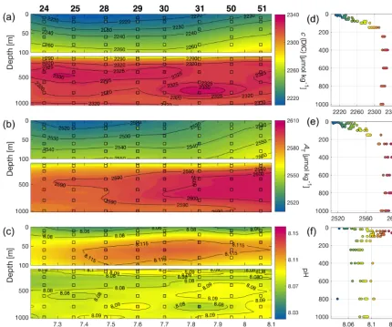
Figure 5.Optimally interpolated fields of(a)dissolved inorganic carbon (c(DIC)),(b)total alkalinity (AT), and(c)pH derived usingc(DIC) andATare displayed along with their depth profiles(d–f). These parameters were sorted into 0.1◦longitude×20 m bins, and the radius of influence used for optimal interpolation was 0.3◦longitude×200 m forc(DIC) and (AT) and 0.3◦longitude×80 m for pH. The water sample values retrieved during the eight CTD casts (displayed in Fig. 1) used for optimal interpolation are superimposed on the interpolated fields as squares.
that the decrease in pH was not caused by changing envi-ronmental conditions. Particularly, one might expect c(O2)
to have a similar pattern to pH if it were related to photosyn-thesis or respiration due to variations in p(CO2) (Cornwall
et al., 2013; Copin-Montégut and Bégovic, 2002). However, c(O2) remained relatively constant throughout the day at all
depth ranges, implying that the level of biological activity in the Sardinian Sea did not change on average throughout the day and hence would not have caused this reduction in pHg.
The decrease in pHgcoincided with increased levels of
so-lar irradiance (Fig. 8a) recorded at meteorological buoy M1 (Fig. 1) during the day at the surface; hence it was likely a light-induced instrumental artefact. The effect of light on the voltage output of FET-based sensors using SiO2- and Si3N4
-sensitive layers is known (Wlodarski et al., 1986), as the presence of photons can excite electrons in the valence band of the semiconductor material, creating holes and allowing
the flow of electrons to the conduction band. This increases the voltage threshold to falsely measure higher hydrogen ion activity, leading to lower apparent pH (Liao et al., 1999).
The effect of light on our sensor was investigated further by exposing two ISFET pH sensors to artificial light whilst placed in reference buffer solutions (TRIS and AMP) un-der laboratory conditions. The results (not shown here) con-firmed that our ISFET sensor is affected by light. The light-induced offset depended on the strength and type of the light source and which sensor was being used. The offset remained relatively constant whilst the light was turned on. Maximum pH offsets of−0.7 (−6×10⁶counts) and−0.15 (−3×10⁶ counts) were found when the LED and halogen lights were used, respectively.
be-Figure 6.A comparison between the measurements retrieved by the glider and those obtained by the ship CTD package. The binned means (red) calculated using glider measurements (grey) are compared with the binned means of the CTD casts obtained from the entire REP14-MED observational domain (blue) and the binned mean values obtained from water samples (SBE oxygen optode sensor for dissolved oxygen concentrations (c(O2)) during the eight CTD casts in Fig. 1 (white) for(a)potential temperature (θ),(b)salinity, and(c)c(O2). Standard deviations (calculated for every 10 m bin) are displayed as error bars in this figure every 30 m for glider and CTD measurements and at every sampled depth for water samples.
Figure 7.The pH obtained by the glider ISFET sensor (pHg; grey) is compared with the depth-binned mean of these profiles (red) along with the corresponding standard deviation error bars (using 10 m bins) displayed in this figure every 30 m. The mean pH values obtained by the ship (pHs) during the eight CTD casts displayed in Fig. 1 are shown (white), with their relevant standard deviations dis-played as error bars. The mean pHgvalues and their corresponding standard deviations were calculated using 10 m depth bins, whereas the mean pHs values and standard deviations were calculated at each sampled depth.
tween 05:00 and 21:00 LT, representing roughly 5 % of all pHgmeasurements, were not used in later analysis. In order
to reduce this light effect on pH measurements in future, IS-FET sensors will have to be placed on the underside of the glider or equipped with a light shield.
Comparing pHgto pHs indicated that the range observed
by the ISFET sensor was much larger. It could be argued that this difference in range is due to the differing temporal and spatial resolution between the glider and the ship mea-surements. However, comparing pHgfurther with pH
mea-surements in the literature on a similar timescale and spa-tial scale (Álvarez et al., 2014) suggests that this is not an issue with resolution. The pHT,25 collected in the western
Mediterranean Sea over a period of around 2 weeks (Álvarez et al., 2014), which is comparable in length to this trial, var-ied by roughly 0.02 at the surface and by around 0.08 at depths greater than 100 m. The range observed by the glider ISFET sensor was therefore 13 times larger at the surface and roughly 3 times larger at depths below 100 m. This dif-ference in range cannot be explained by the high sampling frequency of the glider. Furthermore, the larger variations in pHgwere not a result of changing environmental conditions,
as evidenced by the relatively stablec(O2), θ, and salinity
character-436 M. P. Hemming et al.: Measuring pH using an experimental sensor in the Sardinian Sea
Figure 8. (a)Solar irradiance measured using a pyranometer on meteorological buoy M1 (Fig. 1).(b)Glider-retrieved pH (pHg),(c)dissolved oxygen concentrations (c(O2)),(d)potential temperature (θ), and(e)salinity average anomalies (calculated by subtracting the all-time mean from the hourly means within a given depth interval) for each hour of the day in local time (LT) for five near-surface depth ranges:<5 m, 5–10, 10–15, 15–20, and 20–50 m, as well as two deeper depth ranges of 50–100 and 100–1000 m for both ascending (upward triangle) and descending (downward triangle) dive profiles. The grey shaded area represents the nighttime, whilst the lightly shaded area represents the daytime.
istics (Shitashima et al., 2002, 2013; Shitashima, 2010). Fur-thermore, comparing ISFET measurements with the pHsand
pH presented by Álvarez et al. (2014) suggests that the ac-curacy of the sensor was not as good as previously claimed (Shitashima et al., 2002). Therefore, it was necessary to cor-rect the pHgmeasurements for instrumental drift,
tempera-ture, and pressure.
The response of the ISFET sensor can be described by the Nernst equation (Eq. 1), which relates sensor voltage to hy-drogen ion activity:
E=E∗−mNlg(a(H+) a(Cl−)), (1)
which incorporates the Nernst slope (Eq. 2),
mN=RTln(10)/F, (2)
where T is temperature (K), R is the gas constant (8.3145 J K−1mol−1), F is the Faraday constant (96 485 C mol−1), a(H+) and a(Cl−) are the proton
and chloride ion activities,Eis the measured voltage by the sensor (i.e. electromotive force), and E∗ is representative of the two half-cells in the ISFET sensor forming a circuit (i.e. interface potential) (Martz et al., 2010). It is known that temperature and pressure have an effect onE∗ (strong linear relationship) and that the Nernst slope is a function of temperature. Studies have also shown that it is possible for ISFET sensors to experience some form of hysteresis as a result of changingT and pressure (Martz et al., 2010; Bresnahan et al., 2014; Johnson et al., 2016).
The first step in correcting pHgaimed to reduce the
mea-sured extent of variability to within the meamea-sured limits of pHs. This in part removed the non-monotonous
Figure 9.Salinity(a), dissolved oxygen concentrations (c(O2))(b), and the calculated pH offset values(c)as a function of time at the depth where the in situ temperature was 14±0.1◦C.
(Eq. 3) using the difference between the mean pHsand each
pHg dive measurement where the in situ temperature was
14.0◦C, as water with this temperature was situated at a depth below the thermocline for most dives where the density gradient was weak:
pHOffset=pHs(T )mean−pHg(T ) for T =14±0.1
◦
C. (3)
The calculated offset values as a function of time were compared with salinity andc(O2) where the in situ
tempera-ture was constant at 14◦C (Fig. 9). Variability in salinity and c(O2) with time were strongly related (r2=0.97), whereas
the relationship between pH offset values, salinity, andc(O2),
were not (r2 of around 0.2). Furthermore, the majority of the offset values were calculated below 100 m (Fig. 12d–f) where the density and pH gradients were weak. This indi-cated that our depth-constant time-varying offset correction decreased the apparent range of pH variability by an amount that was mostly associated with instrumental drift rather than physical and biogeochemical variability. Applying these off-sets to the data decreased the range of pH measured by the IS-FET sensor by approximately two-thirds (Fig. 11), with new pHg standard deviations ranging between 0.009 and 0.048
within the top 150 m and between 0.008 and 0.017 at greater depths.
After applying this offset correction, pHgwas further
cor-rected for in situ temperature and pressure using linear re-gression models. The method is outlined below.
1. Calculate 1pH (Eq. 4) as the difference between the mean pHsand pHg:
1pH=pHs,mean−pHg. (4)
2. Determine the line of best fit between1pH and in situ temperature in the top 100 m of the water column where
the temperature gradient was the strongest using linear regression.
3. Correct pHgfor in situ temperature for the entire water
column using the slope (m) and intercept (c) coefficients of the best fit line in step 2 to obtain pHg,tc, where “tc”
stands for “temperature-corrected” values.
4. Calculate the difference between pHg,tc profiles and
mean pHs, producing1pHtc, using an equation similar
to Eq. (4).
5. Determine the line of best fit between1pHtcand
pres-sure for the lower 900 m of the water column using lin-ear regression.
6. Correct pHg,tc for pressure for the entire water column
using the coefficientsmandcin a similar way to step 3 to obtain pHg,tpc, where “tpc” stands for
“temperature-and pressure-corrected” values.
The derived equation used for correcting pHgis as follows: pHg,tpc=pHg−0.021t /◦C+4.5×10−5P /dbar+0.261, (5) wheret is in situ temperature andP is pressure. A good fit was found between pHgand in situ temperature, and a
rea-sonable fit was found with pressure (Fig. 10). The standard deviations of pHg,tpcranged between 0.008 and 0.039 in the
top 150 m of the water column and between 0.007 and 0.013 at greater depths, corresponding to a further decrease in ap-parent variability of 13 to 23 and 14 to 31 % respectively (Fig. 11).
Johnson et al. (2016) ran a series of temperature and pres-sure cycling experiments when testing an ISFET pH sen-sor based on the Honeywell Durafet ISFET. They found a temperature sensitivity of around∂pH/ ∂T = −0.018 K−1, which is similar to our calculated slope, and a pressure hys-teresis of 0.5 mV (pH of around 0.01) at maximum compres-sion (2000 dbar). This is equivalent to a pressure sensitivity of roughly ∂pH/ ∂P =5×10⁻⁶dbar−1, which is an order of magnitude smaller than in this study. This difference in pressure sensitivity could be related to the different housing materials used, as Johnson et al. (2016) used polyether ether ketone (PEEK), whereas acrylic resin was used for our sen-sor.
Salinity covaries with temperature and pressure, and some of the salinity dependence of the offset between pHsand pHg
might have been misattributed to the regression coefficients associated with temperature and pressure. The sensor char-acteristics should therefore be studied in detail under con-trolled laboratory conditions. However, for the purposes of calibrating the high-resolution poor-accuracy measurements (relative to pHs) obtained from the ISFET pH sensor, the
438 M. P. Hemming et al.: Measuring pH using an experimental sensor in the Sardinian Sea
Figure 10.Linear regression fits are displayed for(a)1pH (the difference between the mean pHs and pHgcorrected for drift) vs. in situ temperature in the top 100 m of the water column and(b)1pH corrected for in situ temperature (1pHtc) vs. pressure between 100 and 1000 m using all available dives. Ther2, root mean square error (RMSE), and the equation of the line are displayed for each linear fit.
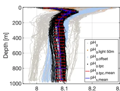
Figure 11. Profiles of glider-retrieved pH (pHg) pre-correction (grey) with a depth-constant time-varying offset correction applied (light blue) and further corrected for in situ temperature and pres-sure (black). The pHg measurements affected by light in the top 50 m of the water column (orange) and not used for the drift; tem-perature and pressure corrections are also shown. The depth-binned mean profile of drift, temperature, and pressure-corrected (tpc) pHg (using 10 m bins) is shown in the foreground (red) along with the standard deviation ranges displayed every 40 m in this figure. The depth-binned mean profile of the pH measurements retrieved by ship (pHs) is plotted for comparison (dark blue) with standard devi-ation ranges displayed at each sampled depth.
3.2.3 Coast to open ocean high-resolution
hydrographic and biogeochemical variability Spatial and temporal variability can be seen in pHg,tpc for
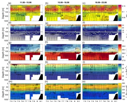
three individual east–west transects using measurements ob-tained within different time periods (Fig. 12a–c). This pH variability is likely related to the air–sea exchange of car-bon dioxide (weak), changes in temperature (indirectly), and biological activity (Yao et al., 2016). In the top 100 m, pH higher than 8.12 was found at depths ranging from 20 to 95 m, whereas lower pH values ranging from 8.06 to 8.09
were present closer to the surface at some locations (e.g. between 7.5 and 7.7◦E and east of 8◦E). The pH maxima were found at depths between 40 and 70 m where θ was around 15◦C (Fig. 12d–f) within the pycnocline (Fig. 12j– l). This band of high pH situated at 20 to 95 m of depth cor-responded with a thick layer ofc(O2)-rich water at similar
depths (Fig. 12m–o). The pH and c(O2) in the top 200 m
of the water column more or less followed isopycnal sur-faces at a range of points in time and space. For example, the slanted isopycnals closer to the coast (east of 7.95◦E) asso-ciated with geostrophic shear corresponded with horizontal gradients in pH andc(O2). Below 100 m,c(O2) decreased to
a minimum of<170 µmol kg−1; although not spatially
ho-mogeneous, this corresponded with generally colder, saltier, and lower-pH waters.
All three east–west transects can be separated into two parts roughly either side of 7.7◦E for depths greater than 100 m. Lower pH values between 8.05 and 8.1 were found in the western part, whereas a higher pH ranging from 8.07 to 8.12 was found in the eastern part, which was partially seen in the pHs measurements (Fig. 5). The spatial
variabil-ity in these eastern and western parts differed for each of the three time periods (times labelled in Fig. 12) with both the eastern high and western low pH patches changing in size vertically and horizontally, corresponding to spatial changes inθ and salinity. Furthermore, salinity,θ, and c(O2) were
lower in the western part compared with the values found at similar depths in the eastern section (Fig. 12d–i, m–o).
In the top 100 m of the water column, the variability in pH andc(O2) is likely related to biological activity and air–sea
gas exchange. As discussed in Sect. 3.1, a DCM within this depth range is common in the Mediterranean Sea when wa-ters are thermally stratified and sufficient nutrients and light are available below the mixed layer (Estrada, 1996). High chlorophyll fluorescence was observed by the ship’s sensor here (Fig. 4d). Enhanced c(O2) values at these depths are
Figure 12.Objectively mapped transects of glider-retrieved(a–c)pH corrected for drift, temperature, and pressure (pHg,tpc).(d–f)Potential temperature (θ),(g–i)salinity,(j-l)potential density anomalies (σθ), and(m–o)dissolved oxygen concentrations (c(O2)) for three different time periods between 11 and 15, 15 and 18, and 18 and 23 June 2014. The spatial ranges of pH measurements affected by light and removed prior to corrections are represented by small white points(a–c). The depth–longitude points at which pH offsets were calculated at a temperature of 14◦C are indicated by pale blue points(d–f). Glider measurements were sorted into 0.04◦longitude×2 m bins, and the radius of influence used for optimal interpolation was 0.1◦longitude×10 m. Glider measurements used for optimal interpolation are superimposed on the interpolated fields for reference.
values are likely the result of changes in the carbon equilib-rium due to the consumption of CO2(Cornwall et al., 2013;
Rivaro et al., 2010; Copin-Montégut and Bégovic, 2002). A similar relationship between pH and primary production was described by Álvarez et al. (2014) in the western Mediter-ranean Sea. As discussed in Sect. 3.1, the fresher waters found in the top 100 m are likely MAW.
The difference in pH between the eastern and western parts at depths greater than 100 m depth highlighted the variabil-ity of water masses in this region. In particular, the higher pH found in the eastern part of the transect (east of 7.7◦E), coinciding with highATandc(DIC) (Fig. 5), was likely
re-lated to the flow of LIW, as described in Sect. 3.1. The LIW flows from the eastern Mediterranean basin (east of the Strait of Sicily) where pH is higher than in the western Mediter-ranean basin (Álvarez et al., 2014) towards the west along the continental shelf edge (Millot, 1999). This high pH found
in the eastern section of the glider transect may therefore be a remnant of these eastern Mediterranean waters. The low-pH low-c(O2) waters found deeper than 100 m result from
increased respiration and remineralisation of organic matter (Lefèvre and Merlivat, 2012), coinciding with higher levels ofc(DIC) deeper than 200 m (Merlivat et al., 2015), which may have been more prominent in the western part of the transect (west of 7.7◦E) leading to decreased levels of pH.
The pycnocline shallowed east of 7.7◦E in the top 100 m
of the water column during all three time periods (times la-belled in Fig. 12), which corresponded with shoaling, high-salinity, low-pH, low-c(O2) waters and highc(DIC),AT, and
440 M. P. Hemming et al.: Measuring pH using an experimental sensor in the Sardinian Sea
However, the mean wind speed was only 2 m s−1, which is weak. On the other hand, salinity maxima seen at depths of 200 to 700 m seem to suggest an intrusion of LIW westward. An intrusion of water away from the coast towards the open ocean has been shown to increase divergence in regions close to shore with strong alongshore currents (Roughan et al., 2005). Upwelling signatures at this longitudinal range along the Sardinian coast have been simulated, particularly in the summer, by Olita et al. (2013) using a hydrodynamic 3-D mesoscale-resolving numerical model. They suggest that a mixture of both current flow and wind preconditioned and enhanced upwelling in this region, which may have also been the case during our deployment. Furthermore, chlorophyll fluorescence (Fig. 4) obtained by ship was higher closer to shore, which is indicative of a greater abundance of biomass in the top 100 m, perhaps fuelled by upwelled nutrients (Porter et al., 2016; El Sayed et al., 1994).
4 Conclusions
Our trials of an experimental pH sensor in the Mediterranean Sea uncovered instrumental problems that were unexpected and will need to be addressed in future usage. These are sum-marised here.
1. The data retrieved from the dual pH–p(CO2) integrated
sensor and from thep(CO2) unit of the stand-alone dual
sensor could not be used due to quality issues. It is un-clear why there was a problem with the measurements obtained by the stand-alonep(CO2) unit; however, we
think the regular on/off cycling of power to the inte-grated dual pH–p(CO2) sensor between sampling did
not allow it to function properly. In future, we would suggest the addition of backup batteries to supply elec-tricity to the sensor between sampling.
2. The stand-alone pH sensor was subject to drift. This could be reduced by subtracting a depth-constant time-varying offset from each dive using the difference be-tween pHgand pHsat a more dynamically stable depth,
but such an approach is not generally recommended or valid. We think that a change in E∗ between the two n-type silicon parts of the semiconductor might be the cause of the drift. To elucidate this drift further, in fu-ture two ISFET sensors should be tested in laboratory conditions within a bridge circuit to attempt to isolate possible factors contributing to drift. Focussing on the root cause of the sensor drift rather than correcting the pH data for drift after the deployment would be more beneficial to the long-term study of ISFET pH–p(CO2)
sensors.
3. The sensor was apparently affected by temperature and pressure, but it is unclear to what extent the empirical relationship between in situ temperature and 1pH in
the thermocline (top 100 m) and between pressure and 1pHtc in the deeper water (100–900 m) can be
gener-alised.
4. The effect of light caused the sensor to measure lower levels of pHgin surface waters. This effect is expected
to be ubiquitous wherever the sensor nears the surface during daytime. In future, the sensor will have to be po-sitioned on the underside of the glider or equipped with a light shield to limit the effect of the sun when close to the surface.
Despite the overall disappointing performance, we were able to demonstrate the potential use of the corrected glider pH measurements to uncover the biogeochemical variability associated with biological and physical mesoscale features. The pHg corrected for drift, temperature, and pressure was
compared temporally and spatially with the other physical and biogeochemical parameters obtained by the glider. This comparison indicated that the pH in the top 100 m of the wa-ter column was mostly related to biological activity where c(O2) was high. Below 100 m, low pH west of 7.7◦E was
likely linked to the remineralisation of organic matter, whilst east of this point, higher pH may have been transported from the eastern Mediterranean basin via LIW. Shoaling isopyc-nals east of 7.7◦E closer to shore may have been indicative
of upwelling, and possible upwelling signatures at the same location could be seen in salinity,θ, pH,c(O2),c(DIC),AT,
and chlorophyll fluorescence.
Data availability. All REP14-MED experiment data are
avail-able on the CMRE data server at http://geos3.cmre.nato.int/ portal/ (NATO Centre for Maritime Research and Experimentation (CMRE), 2016). The data are NATO UNCLASSIFIED and avail-able only for the partners of the experiment. However, interested institutions can sign up for partnership at any time. Requests may be directed to the author or to [email protected].
Competing interests. The authors declare that they have no conflict
of interest.
Acknowledgements. The authors would like to thank all the
partners who helped make REP14-MED a success: the engineers, technicians, and scientists onboard the NRVAllianceand the NRV
Planet, those on land responsible for the logistics of the experiment,
Edited by: J. Chiggiato
Reviewed by: three anonymous referees
References
Álvarez, M., Sanleón-Bartolomé, H., Tanhua, T., Mintrop, L., Luchetta, A., Cantoni, C., Schroeder, K., and Civitarese, G.: The CO2system in the Mediterranean Sea: a basin wide perspective, Ocean Sci., 10, 69–92, doi:10.5194/os-10-69-2014, 2014. Aßmann, S., Frank, C., and Körtzinger, A.: Spectrophotometric
high-precision seawater pH determination for use in underway measuring systems, Ocean Sci., 7, 597–607, doi:10.5194/os-7-597-2011, 2011.
Bates, N. R., Best, M. H. P., Neely, K., Garley, R., Dickson, A. G., and Johnson, R. J.: Detecting anthropogenic carbon dioxide uptake and ocean acidification in the North Atlantic Ocean, Bio-geosciences, 9, 2509–2522, doi:10.5194/bg-9-2509-2012, 2012. Binetti, U.: Dissolved oxygen-based annual biological production from glider observations at the Porcupine Abyssal Plain (North Atlantic), Ph.D. thesis, University of East Anglia, 2016. Bittig, H. C., Fiedler, B., Scholz, R., Krahmann, G., and Körtzinger,
A.: Time response of oxygen optodes on profiling platforms and its dependence on flow speed and temperature, Limnol. Oceanogr. Methods, 12, 617–636, 2014.
Bresnahan, P. J., Martz, T. R., Takeshita, Y., Johnson, K. S., and LaShomb, M.: Best practices for autonomous measurement of seawater pH with the Honeywell Durafet, Methods Oceanogr., 9, 44–60, 2014.
Byrne, R. H. and Breland, J. A.: High precision multiwavelength pH determinations in seawater using cresol red, Deep Sea Res. A, 36, 803–810, 1989.
Copin-Montégut, C. and Bégovic, M.: Distributions of carbonate properties and oxygen along the water column (0–2000 m) in the central part of the NW Mediterranean Sea (Dyfamed site): influ-ence of winter vertical mixing on air–sea CO2and O2exchanges, Deep Sea Res. II, 49, 2049–2066, 2002.
Cornwall, C. E., Hepburn, C. D., McGraw, C. M., Currie, K. I., Pilditch, C. A., Hunter, K. A., Boyd, P. W., and Hurd, C. L.: Di-urnal fluctuations in seawater pH influence the response of a cal-cifying macroalga to ocean acidification, Proc. Roy. Soc. London B, 280, 20132 201, 2013.
Dickson, A.: pH scales and proton-transfer reactions in saline media such as sea water, Geochem. Cosmochim. Acta, 48, 2299–2308, 1984.
Dickson, A. and Millero, F. J.: A comparison of the equilibrium constants for the dissociation of carbonic acid in seawater media, Deep Sea Res. A, 34, 1733–1743, 1987.
Dickson, A. G.: Thermodynamics of the dissociation of boric acid in synthetic seawater from 273.15 to 318.15 K, Deep Sea Res. A, 37, 755–766, 1990.
Dickson, A. G., Sabine, C. L., and Christian, J. R.: Guide to best practices for ocean CO2measurements, PICES Special Publica-tion 3, 191 pp., 2007.
Doney, S. C., Fabry, V. J., Feely, R. A., and Kleypas, J. A.: Ocean acidification: the other CO2problem, Marine Sci., 1, 169–192, 2009.
El Sayed, M. A., Aminot, A., and Kerouel, R.: Nutrients and trace metals in the northwestern Mediterranean under coastal up-welling conditions, Cont. Shelf Res., 14, 507–530, 1994. Eriksen, C. C., Osse, T. J., Light, R. D., Wen, T., Lehman, T. W.,
Sabin, P. L., Ballard, J. W., and Chiodi, A. M.: Seaglider: A long-range autonomous underwater vehicle for oceanographic research, Oceanic Engineering, IEEE Journal of, 26, 424–436, 2001.
Estrada, M.: Primary production in the northwestern Mediterranean, Scientia Marina, 60, 55–64, 1996.
Fabry, V. J., Seibel, B. A., Feely, R. A., and Orr, J. C.: Impacts of ocean acidification on marine fauna and ecosystem processes, ICES Journal of Marine Science: Journal du Conseil, 65, 414– 432, 2008.
Frajka-Williams, E., Eriksen, C. C., Rhines, P. B., and Harcourt, R. R.: Determining vertical water velocities from Seaglider, J. Atmos. Ocean. Tech., 28, 1641–1656, 2011.
Garau, B., Ruiz, S., Zhang, W. G., Pascual, A., Heslop, E., Kerfoot, J., and Tintoré, J.: Thermal lag correction on Slocum CTD glider data, J. Atmos. Ocean. Tech., 28, 1065–1071, 2011.
Hofmann, G. E., Smith, J. E., Johnson, K. S., Send, U., Levin, L. A., Micheli, F., Paytan, A., Price, N. N., Peterson, B., Takeshita, Y., Matson, P. G., Crook, E. D., Kroeker, K. J., Gambi, M. C., Rivest, E. B., Frieder, C. A., Yu, P. C., and Martz, T. R.: High-frequency dynamics of ocean pH: a multi-ecosystem comparison, PloS one, 6, e28983, doi:10.1371/journal.pone.0028983, 2011.
Johnson, K. M., King, A. E., and Sieburth, J. M.: Coulomet-ric TCO2analyses for marine studies; an introduction, Marine Chem., 16, 61–82, 1985.
Johnson, K. S., Jannasch, H. W., Coletti, L. J., Elrod, V. A., Martz, T. R., Takeshita, Y., Carlson, R. J., and Connery, J. G.: Deep-Sea DuraFET: A pressure tolerant pH sensor designed for global sensor networks, Anal. Chem., 88, 3249–3256, 2016.
Key, R. M., Tanhua, T., Olsen, A., Hoppema, M., Jutterström, S., Schirnick, C., van Heuven, S., Kozyr, A., Lin, X., Velo, A., Wal-lace, D. W. R., and Mintrop, L.: The CARINA data synthesis project: introduction and overview, Earth Syst. Sci. Data, 2, 105– 121, doi:10.5194/essd-2-105-2010, 2010.
Knoll, M., Benecke, J., Russo, A., and Ampolo-Rella, M.: Com-parison of CTD measurements obtained by NRV Alliance and RV Planet during REP14-MED, Technical Report WTD71-0083/2015 WB 34 pp., 2015b.
Le Quéré, C., Moriarty, R., Andrew, R. M., Peters, G. P., Ciais, P., Friedlingstein, P., Jones, S. D., Sitch, S., Tans, P., Arneth, A., Boden, T. A., Bopp, L., Bozec, Y., Canadell, J. G., Chini, L. P., Chevallier, F., Cosca, C. E., Harris, I., Hoppema, M., Houghton, R. A., House, J. I., Jain, A. K., Johannessen, T., Kato, E., Keel-ing, R. F., Kitidis, V., Klein Goldewijk, K., Koven, C., Landa, C. S., Landschützer, P., Lenton, A., Lima, I. D., Marland, G., Mathis, J. T., Metzl, N., Nojiri, Y., Olsen, A., Ono, T., Peng, S., Peters, W., Pfeil, B., Poulter, B., Raupach, M. R., Regnier, P., Rö-denbeck, C., Saito, S., Salisbury, J. E., Schuster, U., Schwinger, J., Séférian, R., Segschneider, J., Steinhoff, T., Stocker, B. D., Sutton, A. J., Takahashi, T., Tilbrook, B., van der Werf, G. R., Viovy, N., Wang, Y.-P., Wanninkhof, R., Wiltshire, A., and Zeng, N.: Global carbon budget 2014, Earth Syst. Sci. Data, 7, 47–85, doi:10.5194/essd-7-47-2015, 2015.
esti-442 M. P. Hemming et al.: Measuring pH using an experimental sensor in the Sardinian Sea
mated from a moored buoy, Global Biogeochem. Cy., 26, doi:10.1029/2010GB004018, 2012.
Liao, H.-K., Wu, C.-L., Chou, J.-C., Chung, W.-Y., Sun, T.-P., and Hsiung, S.-K.: Multi-structure ion sensitive field effect transistor with a metal light shield, Sensors and Actuators B: Chemical, 61, 1–5, 1999.
Martz, T. R., Carr, J. J., French, C. R., and DeGrandpre, M. D.: A submersible autonomous sensor for spectrophotometric pH mea-surements of natural waters, Anal. Chem., 75, 1844–1850, 2003. Martz, T. R., Connery, J. G., and Johnson, K. S.: Testing the Honey-well Durafet® for seawater pH applications, Limnol. Oceanogr. Methods, 8, 172–184, 2010.
McNeil, C. L. and D’Asaro, E. A.: A calibration equation for oxy-gen optodes based on physical properties of the sensing foil, Lim-nol. Oceanogr. Methods, 12, 139–154, 2014.
Mehrbach, C., Culberson, C., Hawley, J., and Pytkowics, R.: Mea-surement of the apparent dissociation constants of carbonic acid in seawater at atmospheric pressure, Limnol. Oceanogr., 18, 40 pp., 1973.
Merlivat, L., Boutin, J., and Antoine, D.: Roles of biological and physical processes in driving seasonal air–sea CO2flux in the southern ocean: new insights from CARIOCA pCO2, J. Marine Syst., 147, 9–20, 2015.
Millero, F. J.: Thermodynamics of the carbon dioxide system in the oceans, Geochim. Cosmochim. Acta, 59, 661–677, 1995. Millot, C.: Circulation in the western Mediterranean Sea, J. Marine
Syst., 20, 423–442, 1999.
Mintrop, L., Pérez, F. F., González-Dávila, M., Santana-Casiano, M., and Körtzinger, A.: Alkalinity determination by potentiom-etry: Intercalibration using three different methods, Ciencias Marinas, 26, 23–37, 2000.
NATO Centre for Maritime Research and Experimentation (CMRE): Geo Spatial Data Portal, available at: http://geos3. cmre.nato.int/portal, last access: May 2016.
Olita, A., Ribotti, A., Fazioli, L., Perilli, A., and Sorgente, R.: Sur-face circulation and upwelling in the Sardinia Sea: A numerical study, Cont. Shelf Res., 71, 95–108, 2013.
Onken, R., Fiekas, H.-V., Beguery, L., Borrione, I., Funk, A., Hem-ming, M., Heywood, K. J., Kaiser, J., Knoll, M., Poulain, P.-M., Queste, B., Russo, A., Shitashima, K., Siderius, M., and Thorp-Küsel, E.: High-Resolution Observations in the Western Mediter-ranean Sea: The REP14-MED Experiment, Ocean Sci. Discuss., doi:10.5194/os-2016-82, in review, 2016.
Orr, J. C., Epitalon, J.-M., and Gattuso, J.-P.: Comparison of ten packages that compute ocean carbonate chemistry, Biogeo-sciences, 12, 1483–1510, doi:10.5194/bg-12-1483-2015, 2015. Piterbarg, L., Taillandier, V., and Griffa, A.: Investigating frontal
variability from repeated glider transects in the Ligurian Current (North West Mediterranean Sea), J. Marine Syst., 129, 381–395, 2014.
Porter, M., Inall, M., Hopkins, J., Palmer, M., Dale, A., Aleynik, D., Barth, J., Mahaffey, C., and Smeed, D.: Glider observations of enhanced deep water upwelling at a shelf break canyon: A mech-anism for cross-slope carbon and nutrient exchange, J. Geophys. Res.-Oceans, 121, 7575–7588, 2016.
Queste, B. Y., Heywood, K. J., Kaiser, J., Lee, G., Matthews, A., Schmidtko, S., Walker-Brown, C., and Woodward, S. W.: Deployments in extreme conditions: Pushing the boundaries
of Seaglider capabilities, in: Autonomous Underwater Vehicles (AUV), 2012 IEEE/OES, 1–7, IEEE, 2012.
Rhein, M., Rintoul, S., Aoki, S., Campos, E., Chambers, D., Feely, R., Gulev, S., Johnson, G., Josey, S., Kostianoy, A., Mauritzen, C., Roemmich, D., Talley, L. D., and Wang, F.: Chapter 3: Ob-servations: Ocean, Climate Change, 255–315, 2013.
Rivaro, P., Messa, R., Massolo, S., and Frache, R.: Distributions of carbonate properties along the water column in the Mediter-ranean Sea: Spatial and temporal variations, Marine Chem., 121, 236–245, 2010.
Roemmich, D. H., Davis, R. E., Riser, S. C., Owens, W. B., Moli-nari, R. L., Garzoli, S. L., and Johnson, G. C.: The argo project. global ocean observations for understanding and prediction of climate variability, Tech. rep., DTIC Document, 2003.
Roughan, M., Terrill, E. J., Largier, J. L., and Otero, M. P.: Observations of divergence and upwelling around Point Loma, California, J. Geophys. Res.-Oceans, 110, C04011, doi:10.1029/2004JC002662, 2005.
Shitashima, K.: Evolution of compact electrochemical in-situ pH-pCO2 sensor using ISFET-pH electrode, in: Oceans 2010 MTS/IEEE Seattle, 1–4, 2010.
Shitashima, K., Kyo, M., Koike, Y., and Henmi, H.: Development of in situ pH sensor using ISFET, in: Underwater Technology, 2002. Proceedings of the 2002 International Symposium on, 106–108, IEEE, 2002.
Shitashima, K., Maeda, Y., and Ohsumi, T.: Development of detec-tion and monitoring techniques of CO2leakage from seafloor in sub-seabed CO2storage, Appl. Geochem., 30, 114–124, 2013. Takeshita, Y., Martz, T. R., Johnson, K. S., and Dickson, A. G.:
Characterization of an ion sensitive field effect transistor and chloride ion selective electrodes for pH measurements in seawa-ter, Anal. Chem., 86, 11189–11195, 2014.
Touratier, F. and Goyet, C.: Impact of the Eastern Mediterranean Transient on the distribution of anthropogenic CO2and first es-timate of acidification for the Mediterranean Sea, Deep Sea Res. I, 58, 1–15, 2011.
Uppström, L. R.: The boron/chlorinity ratio of deep-sea water from the Pacific Ocean, in: Deep Sea Research and Oceanographic Abstracts, vol. 21, 161–162, Elsevier, 1974.
Van Heuven, S., Pierrot, D., Rae, J., Lewis, E., and Wallace, D.: MATLAB program developed for CO2system calculations, ORNL/CDIAC-105b, Carbon Dioxide Inf, Anal. Cent., Oak Ridge Natl. Lab., US DOE, Oak Ridge, Tennessee, 2011. Wlodarski, W., Bergveld, P., and Voorthuyzen, J.: Threshold
volt-age variations in n-channel MOS transistors and MOSFET-based sensors due to optical radiation, Sensors and Actuators, 9, 313– 321, 1986.
Yao, K. M., Marcou, O., Goyet, C., Guglielmi, V., Touratier, F., and Savy, J.-P.: Time variability of the north-western Mediter-ranean Sea pH over 1995–2011, Marine Environ. Res., 116, 51– 60, 2016.
Yates, K. K., Dufore, C., Smiley, N., Jackson, C., and Halley, R. B.: Diurnal variation of oxygen and carbonate system parameters in Tampa Bay and Florida Bay, Marine Chem., 104, 110–124, 2007. Zeebe, R. E. and Wolf-Gladrow, D. A.: CO2in seawater: