https://doi.org/10.5194/esd-8-529-2017
© Author(s) 2017. This work is distributed under the Creative Commons Attribution 3.0 License.
Estimation of the high-spatial-resolution variability in
extreme wind speeds for forestry applications
Ari Venäläinen1, Mikko Laapas1, Pentti Pirinen1, Matti Horttanainen1, Reijo Hyvönen1, Ilari Lehtonen1, Päivi Junila1, Meiting Hou2, and Heli M. Peltola3
1Climate Service Centre, Finnish Meteorological Institute, Helsinki, 00101, Finland
2China Meteorological Administration Training Centre, Beijing 100081, China
3School of Forest Sciences, University of Eastern Finland, Joensuu, 80101, Finland
Correspondence to:Ari Venäläinen ([email protected])
Received: 26 January 2017 – Discussion started: 31 January 2017 Revised: 19 May 2017 – Accepted: 8 June 2017 – Published: 5 July 2017
Abstract. The bioeconomy has an increasing role to play in climate change mitigation and the sustainable de-velopment of national economies. In Finland, a forested country, over 50 % of the current bioeconomy relies on the sustainable management and utilization of forest resources. Wind storms are a major risk that forests are exposed to and high-spatial-resolution analysis of the most vulnerable locations can produce risk assessment of forest management planning. In this paper, we examine the feasibility of the wind multiplier approach for down-scaling of maximum wind speed, using 20 m spatial resolution CORINE land-use dataset and high-resolution digital elevation data. A coarse spatial resolution estimate of the 10-year return level of maximum wind speed was obtained from the ERA-Interim reanalyzed data. Using a geospatial re-mapping technique the data were downscaled to 26 meteorological station locations to represent very diverse environments. Applying a com-parison, we find that the downscaled 10-year return levels represent 66 % of the observed variation among the stations examined. In addition, the spatial variation in wind-multiplier-downscaled 10-year return level wind was compared with the WAsP model-simulated wind. The heterogeneous test area was situated in northern Finland, and it was found that the major features of the spatial variation were similar, but in some locations, there were relatively large differences. The results indicate that the wind multiplier method offers a pragmatic and compu-tationally feasible tool for identifying at a high spatial resolution those locations with the highest forest wind damage risks. It can also be used to provide the necessary wind climate information for wind damage risk model calculations, thus making it possible to estimate the probability of predicted threshold wind speeds for wind damage and consequently the probability (and amount) of wind damage for certain forest stand configurations.
1 Introduction
The forest-based bioeconomy plays an important role in cli-mate change mitigation (Kilpeläinen et al., 2016), and in a forested country like Finland, over 50 % of the current bioe-conomy relies on the sustainable management and utilization of forest resources. In Scandinavia, forest grows relatively slowly, and it takes typically 50–100 years from forest cul-tivation to final harvesting. During this long period the pro-jected climate change (Ruosteenoja et al., 2016) may largely alter the growing conditions, thus affecting the survival and productivity of forests (Kellomäki et al., 2008; Bärring et
loads will decrease in southern but increase in northern Fin-land (Lehtonen et al., 2016a). In the past few decades, wind storms have damaged a significant amount of timber and caused large economic and ecological losses in forestry from central to northern Europe (Schelhaas et al., 2003; Gregow, 2013; Gregow et al., 2011; Reyer et al., 2017). In Finland,
strong winds have damaged over 24 million m3of timber in
different winter and summer storms since 2000 (e.g., Gre-gow et al., 2011; Zubizarreta-Gerendiain et al., 2017). Dur-ing the comDur-ing decades, the risk of wind damage to forests is expected to increase, although the frequency and severity of the storms may not increase (Nikulin et al., 2011; Pryor et al., 2012). This increase is due to the shortening of the frozen soil period, which currently improves tree anchorage during the windiest season of the year from late autumn to early spring (Peltola et al., 1999a; Venäläinen et al., 2001; Kellomäki et al., 2010; Gregow et al., 2011).
In addition to the properties of wind (e.g., speed, direc-tion, gustiness and their duration), the stand and site char-acteristics affect largely the vulnerability to wind damage (Peltola et al., 1999b; Gardiner et al., 2016). In Finnish con-ditions, mature stands adjacent to newly clear-cut areas or recently heavily thinned stands are especially vulnerable to wind damage (e.g., Laiho, 1987; Zubizarreta-Gerendiain et al., 2012). Risks to these forests may be decreased by proper forest management and planning for the spatial and temporal patterns of cuttings in forested areas (Tarp and Helles, 1997; Meilby et al., 2001; Zeng et al., 2004, 2007a; Heinonen et al., 2009; Zubizarreta-Gerendian et al., 2017). Several mech-anistic models that have been built in recent decades al-low the prediction of threshold wind speeds that can up-root or break trees under alternative forest stand configura-tions (e.g., Peltola et al., 1999b, 2010; Gardiner et al., 2000, 2008; Byrne and Mitchell, 2013; Seidl et al., 2014; Dupont et al., 2015). Consequently, based on these predicted thresh-old wind speeds it will be possible to predict the probability (and amount) of wind damage based on local wind charac-teristics if sufficient knowledge about the local wind climate is available (e.g., Gardiner et al., 2008; Blennow et al., 2010; Zubizarreta-Gerendian et al., 2017).
An estimation of the frequency of extreme weather events, like extreme wind speeds, can be accomplished by utilizing extreme value analysis (EVA) methods. These methods en-able to fit their statistical distribution (e.g., Gumbel, Frechet or Weibull distribution) into observations that offer the best estimate of the occurrence probability of the most extreme values of the studied phenomena (e.g., Coles, 2001). The software package, Extremes Toolkit, developed by the Na-tional Center of Atmospheric Research (NCAR), is a widely used example of a tool that can be utilized to produce such a statistical distribution (Gilleland and Katz, 2011). For an accurate estimation of the probability of the occurrence of very extreme events with long return periods (e.g., 50 to 100 years), observations over many decades are needed. Ad-ditional difficulty to gain an accurate estimation of return
levels of extreme wind speeds and wind gusts is caused by a lack of homogeneous wind observation time series due to changes in the measuring conditions and instruments (Laa-pas and Venäläinen, 2017). One possibility of assessing the return levels of extreme wind speed in coarse resolution is to use reanalyzed datasets (e.g., Dee et al., 2011), which are produced by assimilating all available observations in a sys-tematic way. The benefit of these datasets is that they of-fer consistent spatial and temporal resolution over several decades (and hundreds of variables). Reanalyzed datasets are also relatively straightforward to handle from a processing standpoint. Although the quality of these data varies from location to location and from variable to variable, the scale of the magnitude of extreme wind for a coarse spatial scale can indeed be estimated based on them (e.g., Brönniman et al., 2012). From the point of local effects, the ERA-Interim dataset has a relatively coarse spatial resolution of about 80 km and detailed spatial variation cannot be taken into account in such a coarse grid. In addition, the continuous change in the availability of reliable observational data cre-ates limitations and must be taken into account, especially if trend analyses of a change in, for example, wind are made (Dee et al., 2011).
The high-resolution spatial variation in extreme wind speed that is affected by topography and surface character-istics (e.g., Wieringa, 1986) can be considered by apply-ing spatial statistical tools (e.g., Etienne et al., 2010; Jung and Schindler, 2015). Additionally, complex airflow mod-els like WAsP (Mortensen, 2015) and WindSim (http://www. windsim.com/), typically applied for wind power potential predictions, can be used for this purpose. One example of exposure estimation is the detailed aspect method of scor-ing (DAMS), which takes into account the local wind cli-mate, elevation, aspect and topographic exposure (Quine and White, 1993; Hale et al., 2015). DAMS is used in the Forest-GALES (http://www.forestry.gov.uk/forestgales) for estimat-ing the probability of wind speeds that cause damage. GIS-based methods for mapping the most wind damage prone areas have also been introduced (e.g., Talkkari et al., 2000; Zeng et al., 2007b; Schindler et al., 2012; Ruel et al., 2002). A pragmatic and computationally very feasible approach to use to estimate the return levels of extreme wind speeds for large geographical areas with very high spatial resolution is the wind multiplier approach. In this approach, regional wind speeds obtained, for example, from the reanalyzed data (or climate change scenario), are downscaled to local wind speeds to consider the local effects of land cover and topog-raphy (e.g., Jones et al., 2005; Cechet et al., 2012; Yang et al., 2014). By applying GIS tools to detailed land-use data and digital elevation maps, it is also very straightforward to produce the required multipliers.
and high-resolution digital elevation data. First we calculated the return levels of extreme wind speeds using the ERA-Interim reanalyses dataset to each coarse resolution grid box and for eight wind directions (cardinal and sub-cardinal). Based on the elevation data, the wind multiplier depicting the effect of orography on wind speed was processed. Likewise, the multiplier depicting the effect of terrain properties on wind speed was processed for each 20 m grid square. There-after, wind multipliers were used to provide quantitative es-timates of local wind conditions relative to the regional wind
speeds in our 20 km×20 km test area located in northern
Finland and for 26 meteorological observing stations with various surface characteristics in different parts of the coun-try as well. The data processing was done using standard Python, QGIS, and ArcGis software routines. The work was motivated by the fact that fulfilling the increasing needs of forest biomass for the growing forest-based bioeconomy will also require increasing area of thinned and clear-cut areas (Heinonen et al., 2017), thus increasing the wind damage and other risks to these forests. Having reliable high-resolution information on extreme wind speeds expected over forested landscapes will enhance both forest management and plan-ning. The method gives a detailed estimate of the exposure of forest to wind damage. However, it is worth noting that if the coarse resolution data that are been downscaled are bi-ased, then the downscaled data will be biased too. For ex-ample, climate scenarios that often contain biases must be bias-corrected prior to downscaling.
2 Material and methods
2.1 The wind multiplier approach
The wind multiplier approach used here follows the one pre-sented in AS/NZS 1170.2 (2011) and Yang et al. (2014), where terrain properties are taken into account when assess-ing local maximum wind speeds (see Eq. 1). The return level
of regional maximum wind speed (VR) in an open terrain at a
10 m height is downscaled into site-specific maximum wind
speed (Vsite) as follows:
Vsite=VR×Mz×Ms×Mh×Md, (1)
where the three wind multipliers used are the terrain/height
multiplier (Mz), shielding multiplier (Ms) and topographic
(hill-shape) multiplier (Mh). The impact of wind direction is
taken into account using a fourth factor (Md). In our study,
we use a 20 m×20 m grid, which is in line with the CORINE
Land Cover 2012 dataset. It provides information on land cover and land use in 2012, and its changes from 2006 to 2012 (based on the European Gioland 2012 project). Our in-terest is forested landscape (including practically no build-ings or other similar obstacles); therefore, the shielding fac-tor was not considered. The return levels of winds speeds
(VR) were also defined separately for the eight cardinal and
intercardinal wind directions. Thus, there was no need to
cal-culate the direction multiplier (Md).
2.2 Estimation of return level for regional maximum wind speeds
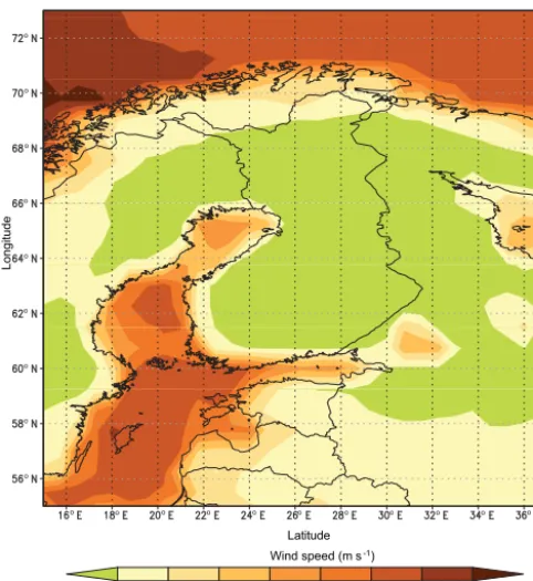
The regional-scale return levels of maximum wind speeds were calculated using the ERA-Interim dataset (Dee et al., 2011) and the generalized extreme value (GEV) method (e.g., Coles, 2001). This method estimated the 10-year re-turn level of maximum wind speed as, for example, in inland
Finland at below 12 m s−1and on the open sea at even around
24 m s−1(Fig. 1). The values are given as grid box averages,
each covering an area of 0.75◦×0.75◦, and the time period
used for the calculation of return levels covered years 1979– 2015. The maximum wind speed dependence on wind direc-tion was estimated by making the calculadirec-tions wind direcdirec-tion wise (Fig. A1). The parameter we analyzed was 10 min in-stantaneous wind speed available at 6 h intervals. The GEV distribution is based on the block maxima approach – i.e., we have maximum values for the selected block, in our cases year, and the distribution is fitted to these data (Coles, 2001). In northern Europe, like in Finland, the cause of the high wind speeds varies from season to season. During summer the extreme wind speed values are typically associated with convective weather phenomena, whereas during winter sea-son they are caused by large synoptic-scale wind storms. As we use only the annual maximum wind speed in the return level calculations we have not paid attention to the cause of the extreme wind speed.
2.3 Estimation of the impact of terrain roughness on maximum wind speeds
In AS/NZS 1170.2 (2011) for elevations below 50 m, 1000 m fetch was used when the surface roughness impact was es-timated. In this study, we applied a somewhat different ap-proach. First, each CORINE land-use class was interpreted to roughness lengths following the technique applied in the pro-duction of the Finnish Wind Atlas (Tammelin et al., 2013). We were interested in this work in very high-resolution spa-tial variation in wind speed in typically highly variable ter-rain mosaic composed of forests, fields, lakes, clear-cut areas etc. The detailed structure of wind flow in this kind of het-erogeneous terrain is very complex (e.g., Dupont and Brunet, 2008). One dominant feature is rapid deceleration of wind when wind encounters a forest edge. In Finnish conditions the main wind damages are found typically within one to two mean stand heights from the upwind forest edge (Pel-tola et al., 1999b). When estimating the impacts of upwind conditions on wind speed in the location that was of inter-est, we used 500 m fetch to calculate the effective
rough-ness (zeff). As the conditions close to the place of interest
Latitude
Longitude
Wind speed (m s )-1
o o o o o o o o o o o
o o o o o o o o o
Figure 1. Ten-year return level of maximum wind speed calcu-lated using ERA-Interim 1979–2015 data and the GEV analysis ap-proach.
presumed to follow normal distribution (Eq. 2) having vari-ance of 150 m. With these assumptions the weighting of each grid is as demonstrated in Fig. A2. The weight of the closest grid square is about 11 % and the furthest grid square located 500 m upwind has a weight of only 0.04 %. This formula is doubtless a simplification of a very complex issue as the ex-act impex-act of roughness elements on wind flow depend, be-side terrain properties also on the characteristics of prevailing air flow. However, when we want to have an application that is computationally so light that it can be utilized easily, all these issues cannot be taken into account and the approach selected here gives a realistic interpretation of the compli-cated issue.
wei=
1
σ √
2πe
−1
2
xi−µ σ
2
, (2)
where σ defines the shape of distribution and, in our case
(150), x is the fetch and µ the location, in this case zero.
Thus,zeffwas calculated as
zeff=
X25
i=1(wei×zoi), (3)
wherezoiis the surface roughness length ofith 20 m grid cell.
The final step to calculate the surface-roughness-dependent
multiplier (Mz) was to use the estimates given in Tables 3.2
and 3.3 by Yang et al. (2014). This step led to an estimate given in Eq. (4).
Mz= −0.056 ln (zeff)+0.7715 (4)
The multipliers were defined for eight directions (cardinal and intercardinal), using the GDAL raster utility programs.
In ERA-Interim analyses, a roughness length for each grid cell is presumed. To normalize the roughness length of the ERA-Interim data into a reference roughness, we multiplied
the ERA-Interim wind speed values by 1/Mz(Eq. 4), using
the ERA-Interim grid cell roughness length as the value of
zeff.
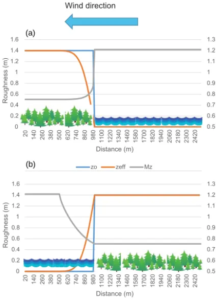
The values ofz0,zeffandMzin the case of sharp roughness
change between forest and lake are demonstrated in Fig. 2.
When the wind comes from an open lake (z0=0.0004 m)
to dense forest (z0=1.4 m), the multiplierMzchanges from
1.21 to 0.75 within a distance of 300 m and to 0.80 within a distance of 80 m. The change is very rapid, demonstrating the strong slowing of wind speed within a dense forest during the first tens of meters. This rapid change is demonstrated in the case where the most vulnerable forest edges are studied; the wind-throw risk is largest within approximately 20–30 m from the upwind edge of a clear-cut area (e.g., Peltola et al., 1999b). The acceleration of wind speed from forest to open
water surface is not as rapid as the slowing; the change inMz
from the minimum value of 0.75 to maximum takes about 500 m (Fig. 2). This rate of acceleration is quite close to the values introduced by Venäläinen et al. (1998). The land-use
map and the values ofZeffandMzfor the Pyhtätunturi Fell
area for northwesterly winds are given in Figs. A3 and A4, respectively.
2.4 Estimation of the impact of topography on maximum wind speeds
The topographic multiplierMhwas taken as the larger of the
two estimatesMh1andMh2(Eq. 5).
Mh1 =0.4343×ln(Heff) for Mh1<1, Mh1 =1 (5a)
Mh2 =0.913×e0.0008Hmsl (5b)
Mh1 simulates the impact of small-scale topographic
varia-tion that is typical in Finland.Heff is calculated as the
dif-ference between the place of interest and the median eleva-tion of 1000 m distance upwind from the locaeleva-tion of interest (see Fig. 3). The logarithmic shape follows that of logarith-mic wind law in the case of surface roughness of 1 m that is
typical for a forest and wind speed 15 m s−1at an elevation
of 10 m. The other multiplier,Mh2, simulates the general
in-crease of wind speed as a function of elevation. The shape of Eq. (5b) is based on an estimate of the dependence of a 50-year return level of maximum wind speed on elevation, defined by using wind measurements made at observing sta-tions located at different elevasta-tions (not published). Finland is a rather flat country, and most of the country is located below an elevation of 200 m a.s.l (above sea level).
Multi-plierMh2is thus larger thanMh1at only very rare locations
in the entire country. The topographic wind multiplierMh
0.5 0.6 0.7 0.8 0.9 1 1.1 1.2 1.3
0 0.2 0.4 0.6 0.8 1 1.2 1.4 1.6
20 140 260 380 500 620 740 860 980
1100 1220 1340 1460 1580 1700 1820 1940 2060 2180 2300 2420
Mz
Roughne
ss
(
m
)
Distance (m)
zo zeff Mz
Wind direction
0.5 0.6 0.7 0.8 0.9 1 1.1 1.2 1.3
0 0.2 0.4 0.6 0.8 1 1.2 1.4 1.6
20 140 260 380 500 620 740 860 980
1100 1220 1340 1460 1580 1700 1820 1940 2060 2180 2300 2420
Mz
Roughne
ss
(
m
)
Distance (m)
zo zef Mz
(a)
(b)
Figure 2.The value of surface roughness lengthsz0andzeffand the
surface-roughness-dependent wind multiplier (Mz) in cases where
wind is from lake to forest(a)and from forest to lake(b).
the Finnish National Data Survey. The data were 25 m spatial resolution raster data re-sampled to 20 m resolution. The data were first smoothed by replacing each pixel with the average
of its 3×3 neighborhood to filter out the very small-scale
noisy features the data might contain. The processing was
done by utilizing the R package “raster”.Heff was then
cal-culated in the eight directions of the wind, using Python and the GDAL routine.
An example of the change in topographic multiplier in the case of a transection reaching over the roughly 500 m high Pyhätunturi Fell (Fig. 5) in northern Finland in the case of northwesterly wind is given in Figs. 4 and A5. As this place is located at a relatively high elevation, the purely on
elevation-dependentMh2dominates, and only in the case of a
steep hill slope around the location interval 11 655–13 405 m
(Fig. 4) does the multiplierMh1get larger values thanMh2.
The approach used in this study is also simpler than the one described in AS/NZS 1170.2 (2011). Still, as the terrain in Finland is relatively flat, the main impact of these relatively small-scale topographic variations can be taken into account even with the schema utilized here.
Figure 3.A visualization of the calculation of the topographic mul-tiplierMh.
2.5 Verification tests
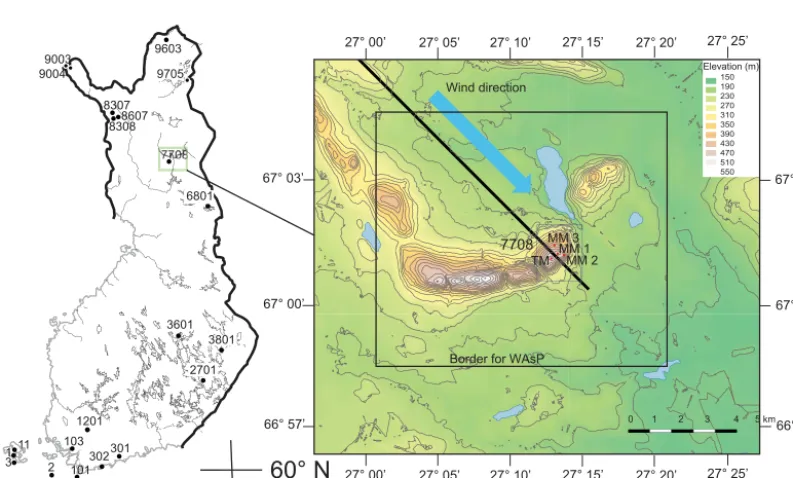
The first verification tests were done by utilizing wind mea-surements made at 26 observing stations in Finland; 23 of these stations belong to the observation network maintained by the Finnish Meteorological Institute (FMI) and represent conditions ranging from open sea to agricultural land, forests, and open hill areas. More detailed analyses were made in
northern Finland (67.02204◦lat, 27.2184◦long) for the
Py-hätunturi Fell test area, with an elevation range of 148– 526 m a.s.l. (Figs. 5, A3). In addition to the forests, other terrain types included open tundra, agricultural fields, lakes, and ski slopes. The test area had both larger topographic variation and spatial variation in wind speeds than the typ-ical Finnish landscape and in that sense represented more challenging conditions than those expected in most of the rest of the country. This Pyhätunturi Fell test area was also used in the EU-funded MOWIE project, where three 10 m tall wind-measuring masts were installed at a range of elevations above the mean sea level: 470 m (MM1), 419 m (MM2) and 408 m (MM3). In addition, there was a permanent observing mast (FMI station number 7708) on the telecommunication mast (TM) at an elevation of 61 m above the surface at the top of the hill (see Fig. 5). All wind speed measurements were corrected to 10 m high values by applying the logarith-mic wind law. Wind climate simulations for this same area have earlier been made utilizing the Karlsruhe Mesoscale Model (KAMM) and WAsP by Frank et al. (1999). An air-borne detailed photograph of the area is available, for ex-ample, from the Finnish Land Survey’s map service (https: //asiointi.maanmittauslaitos.fi/karttapaikka/?lang=en).
0 0.5 1 1.5 2 2.5
-200 -100 0 100 200 300 400 500
35 385 735
1085 1435 1785 2135 2485 2835 3185 3535 3885 4235 4585 4935 5285 5635 5985 6335 6685 7035 7385 7735 8085 8435 8785 9135 9485 9835 10185 10535 10885 11235 11585 11935 12285 12635 12985 13335 13685 14035 14385 14735 15085 Hm
sl
,
Hm
e
d
,
He
ff
(
m
)
Distance (m)
Hmsl Hmed Heff Mh1 Mh2
Mh
Wind direction
Figure 4.Variations in elevation (Hmsl), median elevation (Hmed), and the effective elevation (Heff) (left axis) and topographic multipliers
Mh1 and Mh2 (Eq. 5, Fig. 3) (right axis) along a transection from northwest to southeast (the black line in Fig. 5) crossing the Pyhätunturi Fell in northern Finland.
MM 2 MM 1 MM 3 TM
Elevation (m) 150 190 230 270 310 350 390 430 470 510 550 Wind direction
0 1 2 3 4 5 km 1201
1 2 3
11
101 103 301
8307 83088607 9003
9004
9603
30° E
60° N
100 km
7708
3601 3801
2701
302
6801 9705
Border for WAsP
27° 10’ 27° 15’ 27° 20’ 27° 25’
27° 05’ 27° 00’
27° 10’ 27° 15’ 27° 20’ 27° 25’
27° 05’ 27° 00’
67° 00’ 67° 03’
66° 57’
67° 00’ 67° 03’
66° 57’
In this sense the observational values are not exactly the same as reanalyzed data, and this may create some systematic dif-ference. However, when using the annual maximum values as the bases for fitting the distribution this may reduce the bias. For stations MM1, MM2 and MM3, there was only 2 years of data available, a short period to estimate even 10-year re-turn levels. Therefore, to have the extreme value analysis be as robust as possible, for these stations, we applied the block maxima approach (e.g., Coles, 2001) to the monthly maxi-mum values, using the R package extRemes (Gilleland and Katz, 2016). For most of the other station locations, the data used for the extreme value analyses covered the years 1979– 2015, which is the same period as used in the case of ERA-Interim data.
For the Pyhätunturi Fell area, we also compared a spa-tial variation in high wind speed as simulated by the WAsP package with a wind multiplier downscaled wind. The area was slightly smaller (Fig. 5) due to the availability of ter-rain information needed for a WAsP simulation. In the WAsP simulation, the geostrophic wind speed was expected to be
39 m s−1from northwest. This geostrophic wind speed leads
to approximately 26 m s−1winds at the top of the
Pyhätun-turi Fell, which is roughly the 10-year return level maximum wind speed (see Table 1). For a comparable wind multiplier
downscaling, the coarse-scale northwesterly wind 12.7 m s−1
was used as the basis in the calculation. In this way the max-imum wind speed was the same in both simulations.
3 Results
3.1 Comparison of measurement-based return levels to those based on a wind multiplier approach
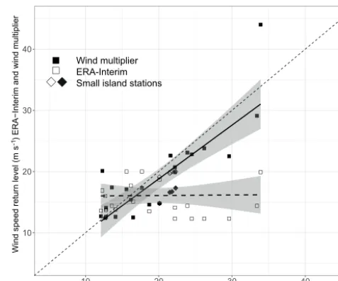
A comparison of the ERA-Interim and wind-multiplier-based assessment of 10-year return levels of wind speed to the esti-mates based on measurements for the test locations (Table 1, Fig. 6) revealed that for these locations, and representing dif-ferent kinds of terrain and elevations, the wind multiplier ap-proach improved the local wind speed return level estimates
remarkably (R2=0.66). There was a small bias in the
esti-mates, the mean difference being−1.2 m s−1and the RMSE
4.09 m s−1. According to the comparison, the wind multiplier
approach tends to underestimate the wind speed on station lo-cated at small Baltic Sea islands – i.e., according to the mea-surements there is less deceleration of wind speed on these islands than predicted by the method (Fig. 6). This indicates that the method exaggerates the impact of change in surface roughness on wind speed in these rather specific conditions. As we are interested in inland and mainly forested landscape, this is not a crucial issue. However, further development of the method is needed in order to also be able to simulate the coastal and island conditions. The largest differences were found in the case of station no. 9004, which is located at an elevation of 1004 m a.s.l., i.e., almost at the highest point in Finland. The anemometer at this station is also located at the
10 20 30 40
10 20 30 40
Wind speed return level (m s ) observations-1
W in d sp ee d re tu rn le ve l ( m s ) E R A − In te ri m a nd w in d m ul tip lie r -1 Wind multiplier ERA-Interim Small island stations
Figure 6.Comparison of 10-year return levels of maximum wind speeds, as calculated, based on observations and by utilizing the wind multiplier method (Eq. 1) and the ERA-Interim dataset for the 26 measuring sites (Fig. 5). Return levels taken directly from the ERA-Interim dataset with no wind multiplier correction are in-cluded in the visualization. The shaded areas are 95 % confidence levels for the linear trend lines depicting the dependence between the datasets. The diamond shape symbols indicate that the station is located on small Baltic Sea islands.
edge of a steep slope, thus leading to a high topographic mul-tiplier value.
At the four Pyhätunturi Fell stations, the wind multiplier estimates were close to the measurement-based estimates with the exception of station MM1. The estimate based on
measurements made at MM1 (29.6 m s−1) was about 5 m s−1
higher than the return level estimate calculated for the tele-com mast at the same height. The difference between MM1
and MM2 was about 3 m s−1. The return level estimates for
stations MM1, MM2 and MM3 were based on 2 years of measurements and also led to a high degree of uncertainty. For example, for station MM1, the estimated 95 %
confi-dence levels were 23.1 to 36.1 m s−1. The corresponding
es-timate of the telecom tower based on 19 years of measure-ments was more robust with 95 % confidence levels, i.e.,
21.5 to 27.6 m s−1.
3.2 Spatial variation in maximum wind speeds
The spatial variation in 10-year return levels of wind speeds
within the roughly 4000 km2Pyhätunturi test area was large.
The lowest values for the 10-year return level were around
9.2 m s−1and the highest on top of the Pyhätunturi Fell were
approximately 26.5 m s−1 (Fig. 7). A crude approximation
indicates that mean 10 min wind speed exceeding 12 m s−1
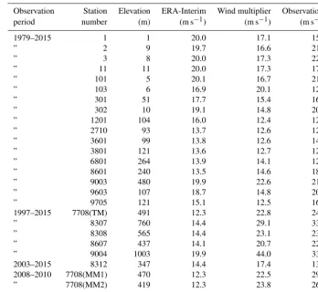
Table 1.Ten-year return levels of maximum wind speed (m s−1) as estimated directly from ERA-Interim data, downscaled to station locations using the wind multiplier approach, and calculated based on measurements for the station locations given in Fig. 5. The observations are corrected to represent 10 m wind speed by applying logarithmic wind profile. Station elevation a.s.l. (m) has been included in the table.
Observation Station Elevation ERA-Interim Wind multiplier Observations
period number (m) (m s−1) (m s−1) (m s−1)
1979–2015 1 1 20.0 17.1 15.6
” 2 9 19.7 16.6 21.5
” 3 8 20.0 17.3 22.3
” 11 11 20.0 17.3 17.7
” 101 5 20.1 16.7 21.8
” 103 6 16.9 20.1 12.3
” 301 51 17.7 15.4 16.2
” 302 10 19.1 14.8 20.1
” 1201 104 16.0 12.4 12.7
” 2710 93 13.7 12.6 12.8
” 3601 99 13.8 12.6 14.1
” 3801 121 13.6 12.7 12.1
” 6801 264 13.9 14.1 12.8
” 8601 240 13.5 14.6 18.7
” 9003 480 19.9 22.6 21.6
” 9603 107 18.7 14.8 20.1
” 9705 121 15.1 12.5 16.5
1997–2015 7708(TM) 491 12.3 22.8 24.5
” 8307 760 14.4 29.1 33.4
” 8308 565 14.4 23.1 23.9
” 8607 437 14.1 20.7 22.2
” 9004 1003 19.9 44.0 33.9
2003–2015 8312 347 14.4 17.4 13.6
2008–2010 7708(MM1) 470 12.3 22.5 29.6
” 7708(MM2) 419 12.3 23.8 26.2
” 7708(MM3) 408 12.3 19.9 22.2
When we looked at the spatial variation in a 10-year return level of wind speed inside the test area, we can see areas
having wind speeds higher than the threshold of 12 m s−1
found on local topographic formations, at the edges of open terrain, and at high-elevation locations. At a total 23.8 % of grid squares, the 10-year return level wind speed reaches the threshold, and if we look only at the forested area, then we end up with 22.8 %. This statistic means that approximately 20 % of the area is exposed to wind speeds that can lead to forest damage. The exact value depends, however, on several factors, including tree and stand characteristics. The next step is to use a wind-throw risk model like HWIND (Peltola et al., 1999b) to simulate the threshold wind speeds needed for wind damage and further to estimate the probability of occur-rence of such winds and the amount of damage, respectively. Unfortunately, in this work we do not have the needed forest inventory data available for the test area enabling the simula-tions. However, this work will be done in future studies using forested areas with sufficient data.
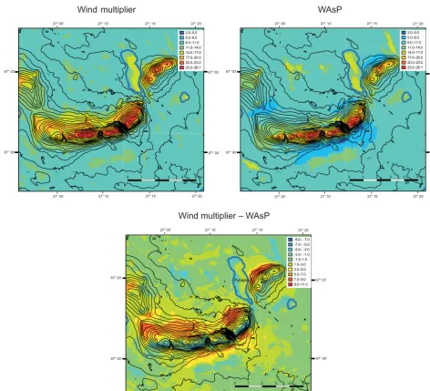
In a qualitative comparison, the wind multiplier approach and a WAsP simulation produced the same dominant features of spatial variation in maximum wind speed; maximum
val-8.0 10.0 12.0 14.0 16.0 18.0 20.0 22.0 24.0 26.0 28.0
27° 10’ 27° 15’ 27° 20’ 27° 25’ 27° 05’
27° 00’
27° 10’ 27° 15’ 27° 20’ 27° 25’ 27° 05’
27° 00’
67° 00’ 67° 03’
66° 57’
67° 00’ 67° 03’
66° 57’ 0 1 2 3 4 5 km
2.0–5.0 5.0–8.0 8.0–11.0 11.0–14.0 14.0–17.0 17.0–20.0 20.0–23.0 23.0–26.1
27° 10’ 27° 15’ 27° 20’ 27° 05’
27° 05’ 27° 10’ 27° 15’ 27° 20’
67° 00’ 67° 03’
67° 00’ 67° 03’
0 1 2 3 4 5 km
2.0–5.0 5.0–8.0 8.0–11.0 11.0–14.0 14.0–17.0 17.0–20.0 20.0–23.0 23.0–26.1
27° 10’ 27° 15’ 27° 20’ 27° 05’
27° 05’ 27° 10’ 27° 15’ 27° 20’
67° 00’ 67° 03’
67° 00’ 67 °03’
0 1 2 3 4 5 km
-9.0– -7.0 -7.0– -5.0 -5.0– -3.0 -3.0– -1.0 -1.0–1.0 1.0–3.0 3.0–5.0 5.0–7.0 7.0–9.0 9.0–11.0 Pyhäjärvi
Pyhäkuru Pikkukuru
27° 10’ 27° 15’ 27° 20’ 27° 05’
27° 05’ 27° 10’ 27° 15’ 27° 20’
67° 00’ 67° 03’
67° 00’ 67° 03’
0 1 2 3 4 5 km m
Wind ult iplier WAsP
Wind multiplier – WAsP
Figure 8.Comparison of the spatial variation in wind speed as estimated, using the wind multiplier approach, calculated using the WAsP program. The last figure depicts the difference between the two methods. Wind direction is from the northwest and in the case of the wind multiplier it is 12.7 m s−1. For the WAsP simulation a geostrophic northwesterly wind of 39.2 m s−1was assumed.
ues were found at treeless fell-top areas (Fig. 8). One inter-esting feature was the case of the WAsP simulation for the ac-celeration of wind at the forest–lake edge; it was immediate, and so was the deceleration on the opposite shore. In such a case of wind multiplier simulation, the impact of roughness change is reflected over a longer distance, as can be seen in the case of the Lake Pyhäjärvi. On top of the fell, the wind
speed was adjusted to approximately the same 26 m s−1. On
the lee side of the top of the fell, the wind multiplier simula-tions indicated a more rapid deceleration of wind speed than WAsP, while on the side to windward, the wind multiplier gave higher wind speeds. With no proper measurements, we could not decide which reflected the real conditions better.
In the case of canyons like Pyhäkuru and Pikkukuru (Fig. 8) WAsP is more capable of predicting higher wind speed val-ues than the wind multiplier and obviously reflect the pre-vailing conditions better. For most of the lower elevation ar-eas, the difference between the two simulations was small, and with these input wind speeds, the prevailing difference is
on the scale of 1 m s−1, with the wind multiplier giving
4 Discussion and conclusions
4.1 Reliability of tested method
The wind multiplier method has been used earlier to esti-mate the design values of buildings and other constructions (AS/NZS 1170.2, 2011) and assessment of wind damage risk (Yang et al., 2014). Based on our study, the wind multiplier method is very capable of identifying the locations having the highest extreme wind speeds in Finnish conditions. This is true despite the fact that this approach is much simpler than the dynamical models. The method seem to underesti-mate wind speeds at small islands located on the open sea and this issue has to be taken into account if high-spatial-resolution assessment of extreme wind speeds is calculated to such conditions. The wind multiplier approach is also eas-ily transferable to any location with needed terrain informa-tion and is an interesting and easily applicable alternative to use to assess the exposure of terrain.
How precise each grid square estimate is depends on sev-eral external factors. First, we must have an estimate of the coarse-scale return levels of the extreme wind speeds. Re-analyzed data give such a coarse estimate. If the reRe-analyzed data are compared to in situ measurements in certain wind storm event, it is easy to find large differences between them. In addition, the return levels of wind speed calculated using ERA-Interim grid values can be quite different from the value based on point measurements, but downscaling the grid value to the point using the wind multiplier approach improves the estimate substantially, as we demonstrated in Fig. 6. It is also good to remember that, although the wind measure-ments made at meteorological stations can go through several quality control steps, they may still contain erroneous values. FMI has a three-stage quality control system. The first check is done at the observation station site checking the main in-strument malfunctions. The next check is done before storing the data in the database. This check includes, for example, comparison with the extreme values and temporal and spatial consistency. The final step is the manual quality control for those values that did not pass earlier steps. The quality con-trol ensures that the values stored in database are realistic and can have occurred. However, quality control does not guar-antee that the measurements are exactly correct. In addition, quality control does not ensure the homogeneity of observa-tions. The changes at measuring site and changes in instru-mentation as well as the changes in the height of anemometer installation can lead to discontinuations, i.e., break points, in observational time series. These break points are relatively common also in wind observational time series like studied by Laapas and Venäläinen (2017). In that sense the return periods based on measured values (Table 1, Fig. 6) contain uncertainties that are wise to remember when the compari-son is fully valued.
The simple visualization and comparison of the spatial variation in wind speed at Pyhätunturi Fell was done by
ap-plying WAsP and, in addition, by apap-plying wind multipliers. These demonstrate that the main features of spatial varia-tion in an extreme wind field produced by these two different methods are very similar. A profound analysis on the exact accuracy of the simulations is not possible, however, based on the available measurements; it would require much more detailed and reliable wind measurement data. However, by fine tuning the wind multipliers, it is possible to achieve re-sults that are closer to the WAsP simulation. Pyhätunturi is not a typical Finnish forested landscape due to its high to-pographic variation. In those parts of the test area that ex-emplify a more typical landscape with only relatively small topographic features and found at elevations below 300 m, these two methods give quite similar results. It is also good to remember that, as we are summarizing all wind directions (Fig. 7), the importance of lee-side wind simulation accuracy is not as crucial as having accuracy for the windward size having the highest wind speeds.
The wind multiplier method itself is also relatively easy to apply. The calculation of surface roughness and topographic multipliers can be done using routine GIS tools, and these calculations can be done for large areas, such as the whole country. Similarly, this method could be used to assess the risks to forests that are related to forest management and planning with relatively little extra effort. Further, climate change impact assessments can be done with high spatial res-olution when the return levels of maximum wind speed are calculated using climate scenarios instead of only reanalyzed data.
One challenge of the method is the accuracy of sur-face roughness information in the CORINE dataset; it is updated approximately every 6 years and thus does not represent real-time land-use conditions for all loca-tions. For example, forest clear-cutting changes the rough-ness conditions very dramatically. Thinning affects it less. More frequent updates to surface conditions could be obtained from satellite measurements. As an example, the European Space Agency’s (ESA) satellite Sentinel-2 (http://www.esa.int/Our_Activities/Observing_the_Earth/ Copernicus/Sentinel-2) is producing high-spatial-resolution (at best 10 m) data describing the earth surface properties. Because of the development of satellite-measured data han-dling methods, the data can provide new possibilities for up-dating the surface state with a higher frequency than, for ex-ample, the CORINE data are updated. Use of up-to-date air-borne laser scanning data, if available (e.g., Kotivuori et al., 2016), can also offer a viable means to provide very detailed information on forest properties and thus also offer informa-tion on surface roughness condiinforma-tions.
4.2 Conclusions
wind damage risks to forests, especially at the upwind edges of new clear-felling areas and in recently thinned stands that have not yet been acclimated to increasing wind load-ing. Thus, proper risk assessment is a clear pre-condition for a sustainable forest-based bioeconomy. This study demon-strated a useful tool to use for forest management and plan-ning.
The tested wind multiplier method is very capable of iden-tifying the locations (at high resolution) having the highest extreme wind speeds and could well support the precise as-sessment of wind damage risks to forests. It can also be used to provide needed wind climate information for wind dam-age risk model calculations. Thus, it would make it possi-ble to estimate the probability of predicted threshold wind speeds for wind damage, and consequently the probability (and amount) of wind damage under certain forest stand con-figurations. Accurate estimations of the spatial variation in the return levels of extreme wind speed with very high spatial resolution over the whole country or even over larger areas like Fennoscandia are possible in the future using this ap-proach. A high-resolution estimation of climate change im-pacts on wind damage risks to forests is also feasible using this approach.
Appendix A
E
N NE SE S SW WNW 10
15 20 25 30 35
E
N NE SE S SW WNW Wind direction 10
15 20 25 30 35
W
in
d
sp
ee
d
(m
s
)
-1
W
in
d
sp
ee
d
(m
s
)
-1
Wind direction ERA-Interim Measurements
(a) (b)
Figure A1.Box plot depicting measured 10 min wind speed values at the Pyhätunturi telecom mast station during years 1997–2016 and as taken from the ERA-Interim. The values measured at an elevation of 61 m were corrected to represent 10 m by applying logarithmic wind law. Only values that are 11.4 m s−1(corresponding value 15 m s−1at elevation of 61 m) are included into the analyses.
Figure A2.The weight of each grid square’s roughness on the effective roughness (zeff) as a function of upwind distance as calculated using
Artificial surfaces Agricultural areas Forests
Shrub and/or herbaceous vegetation associations Open spaces with little or no vegetation Inland wetlands
Inland waters LEGEND
27° 10’ 27° 15’ 27° 20’ 27° 25’
27° 05’ 27° 00’
27° 10’ 27° 15’ 27° 20’ 27° 25’
27° 05’
0 1 2 3 4 5 km
67° 00’ 67° 03’
66° 57’ 67° 00’
67° 03’
66° 57’
Figure A3.Land-use map for the Pyhätunturi Fell area based on the CORINE dataset.
0.0004 0.1000 0.2000 0.3000 0.4000 0.5000 0.6000 0.7000 0.8000 0.9000 1.0000 1.1000 1.2000 1.3000 1.4000 Effective roughness
27° 10’ 27° 15’ 27° 20’
27° 05’
27°05’ 27°10’ 27°15’ 27°20’
67° 00’ 67° 03’
67° 00’ 67° 03’
0.75 0.80 0.85 0.90 0.95 1.00 1.05 1.10 1.15 1.20 1.25 Roughness multiplier
27° 10’ 27° 15’ 27° 20’
27° 05’
27° 05’ 27° 10’ 27° 15’ 27° 20’
67° 00’ 67° 03’
(a) (b)
Figure A4.Effective roughness (zeff, Eq. 4) and roughness-dependent wind multiplier (Mz) calculated for the Pyhätunturi Fell area for
1.0–1.1 1.1–1.2 1.2–1.3 1.3–1.4 1.4–1.5 1.5–1.6 1.6–1.7 1.7–1.8 1.8–1.9 1.9–2.0 2.0–2.1 2.1–2.2 2.2–2.3
27° 10’ 27° 15’ 27° 20’ 27° 05’
27° 05’ 27° 10’ 27° 15’ 27° 20’
67° 00’ 67° 03’
67° 00’ 67° 03’
1.0–1.1 1.1–1.2 1.2–1.3 1.3–1.4 1.4–1.5 1.5–1.6 1.6–1.7 1.7–1.8 1.8–1.9 1.9–2.0 2.0–2.1 2.1–2.2 2.2–2.3
27° 10’ 27° 15’ 27° 20’ 27° 05’
27° 05’ 27° 10’ 27° 15’ 27° 20’
67° 00’ 67 °03’
1.0–1.1 1.1–1.2 1.2–1.3 1.3–1.4 1.4–1.5 1.5–1.6 1.6–1.7 1.7–1.8 1.8–1.9 1.9–2.0 2.0–2.1 2.1–2.2 2.2–2.3
27° 10’ 27° 15’ 27° 20’ 27 °05’
27° 05’ 27° 10’ 27° 15’ 27° 20’
67° 00’ 67° 03’
67° 00’ 67° 03’
Mh1 Mh2
Mhfinal
Figure A5.Topographic wind multipliers (Eq. 6) calculated for the Pyhätunturi Fell area for northwesterly winds.
Competing interests. The authors declare that they have no con-flict of interest.
Special issue statement. This article is part of the special issue “Multiple drivers for Earth system changes in the Baltic Sea re-gion”. It is a result of the 1st Baltic Earth Conference, Nida, Lithua-nia, 13–17 June 2016.
Acknowledgements. This work was supported by the Strategic Research Council at the Academy of Finland, project FORBIO (grant number 293380).
Edited by: Marcus Reckermann Reviewed by: two anonymous referees
References
AS/NZ 1170.2: Australian/New Zealand Standard, Structural de-sign actions, Part 2: Wind actions, 2nd Edn., Wellington, 96 pp., 2011.
Blennow, K., Andersson, M., Sallnäs, O., and Olofsson, E.: Climate change and the probability of wind damage in two Swedish forests, For. Ecol. Manag., 259, 818–830, https://doi.org/10.1016/j.foreco.2009.07.004, 2010.
Bärring, L., Berlin, M., and Gull B. A.: Tailored climate indicators for climate-proofing operational forestry applications in Sweden and Finland, Int. J. Climatol., 37, 123–142, 2017.
Brönnimann, S., Martius, O., von Waldow, H., Welker, C., Luter-backer, J., Compo, G. P., Sardeshmukh, P. D., and Usbeck, T.: Extreme winds at northern mid-latitudes since 1871, Meteorol. Z., 21, 13–27, https://doi.org/10.1127/0941-2948/2012/0337, 2012.
Byrne, K. and Mitchell, S.: Testing of WindFIRM/ForestGALES-BC: a hybrid-mechanistic model for predicting windthrow in partially harvested stands, Forestry, 86, 185–199, https://doi.org/10.1093/forestry/cps077, 2013.
Cechet, R., Sanabria, L., Divi, C., Thomas, C., Yang, T., Arthur, W., Dunford, M., Nadimpalli, K., Power, L., White, C., Bennett, J., Corney, S., Holz, G., Grose, M., Gaynor, S., and Bindoff, N.: Climate Futures for Tasmania: Severe wind hazard and risk tech-nical report, GA Record 2012/43, 2012.
Coles, S.: An introduction to statistical modeling of extreme values, Springer-Verlag, Lontoo, 204 pp., 2001.
Dee, D., Uppala, S., Simmons, A., Berrisford, P., Poli, P., Kobayashi, S., Andrae, U., Balmaseda, M., Balsamo, G., Bauer, P., Bechtold, P., Beljaars, A., van de Berg, L., Bidlot, J., Bor-mann, N., Delsol, C., Dragani, R., Fuentes, M., Geer, A., Haim-berger, L., Healy, S., Hersbach, H., Hólm, E., Isaksen, L., Kåll-berg, P., Köhler, M., Matricardi, M., McNally, A., Monge-Sanz, B. M., Morcrette, J., Park, B., Peubey, C., de Rosnay, P., Tavolato, C., Thépaut, J.-N., and Vitart, F.: The ERA-Interim reanalysis: configuration and performance of the data assimilation system, Q. J. Roy. Meteor. Soc., 137, 553–597, 2011.
Dupont, S. and Brunet, Y.: Impact of forest edge shape on tree stability: a large-eddy simulation study, Forestry, 81, 299–315, https://doi.org/10.1093/forestry/cpn006, 2008.
Dupont, S., Ikonen, V.-P., Väisänen, H., and Peltola, H.: Predicting tree damage in fragmented landscapes using a wind risk model coupled with an airflow model. Can. J. For. Res., 5, 1065–1076, https://doi.org/10.1139/cjfr-2015-0066, 2015.
Etienne, C., Lehman, A., Goyette, S., Lopez-Moreno, J. I., and Beniston, M.: Spatial Predictions of Extreme Wind Speeds over Switzerland Using Generalized Additive Models, J. Appl. Mete-orol. Clim., 49, 1956–1970, 2010.
Frank, H., Petersen, E., Hyvönen, R., and Tammelin, B.: Calcula-tion on the wind climate in Northern Finland: The importance of inversion and roughness variations during the season, Wind Energy, 2, 113–123, 1999.
Gardiner, B., Peltola, H., and Kellomäki, S.: Comparison of two models for predicting the critical wind speeds required to damage coniferous trees, Ecol. Model., 129, 1–23, 2000.
Gardiner, B. A., Byrne, K., Hale, S., Kamimura, K., Mitchell, S. J., Peltola, H., and Rue, J. C.: A review of mechanistic mod-elling of wind damage risk to forests, Forestry, 81, 447–463, https://doi.org/10.1093/forestry/cpn022, 2008.
Gardiner, B., Berry, P., and Moulia, B.: Review: Wind impacts on plant growth, mechanics and damage, Plant Sci., 245, 94–118, https://doi.org/10.1016/j.plantsci.2016.01.006, 2016.
Gilleland, E. and Katz, R. W.: New software to analyze how ex-tremes change over time, Eos, 92.2., 13–14, 2011.
Gilleland, E. and Katz, R. W.: extRemes 2.0: An Extreme Value Analysis Package in R, J. Stat. Softw., 72, 1–39, https://doi.org/10.18637/jss.v072.i08, 2016.
Gregow, H: Impacts of strong winds, heavy snow loads and soil frost conditions on the risks to forests in Northern Europe, Finnish meteorological Institute Contributions, 94, 178 pp., 2013.
Gregow, H., Peltola, H., Laapas, M., Saku, S., and Venäläinen, A.: Combined occurrence of wind, snow loading and soil frost with implications for risks to forestry in Finland under the cur-rent and changing climatic conditions, Silva Fenn., 45, 35–54, https://doi.org/10.14214/sf.30, 2011.
Hale, S., Gardiner, B., Peace, A., Nicoll, B., Taylor, P., and Pizzi-rani, S.: Comparison and validation of three versions of a for-est wind risk model, Environ. Modell. Software, 68, 27–41, https://doi.org/10.1016/j.envsoft.2015.01.016, 2015.
Heinonen, T., Pukkala, T., Ikonen, V.-P., Peltola, H., Venäläi-nen, A., and Dupont, S.: Integrating the risk of wind dam-age into forest planning, For. Ecol. Mandam-age., 258, 1567–1577, https://doi.org/10.1016/j.foreco.2009.07.006, 2009.
Heinonen, T., Pukkala, T., Mehtätalo, L., Asikainen, A., Kangas, J., and Peltola, H.: Scenario analyses for the effects of harvest-ing intensity on development of forest resources, timber supply, carbon balance and biodiversity of Finnish forestry, For. Policy Econ., 80, 80–98, 2017.
Jones, T., Middelmann, M., and Corby, N. (Eds.): Natural hazard risk in Perth, Western Australia, Comprehensive Report, Geo-science Australia, 352 pp., 2005.
Jung, C. and Schindler, D.: Statistical Modeling of Near-surface Wind Speed: A Case Study from Baden-Wuerttemberg (South-west Germany), Austin J. Earth Sci., 2, 1–11, 2015.
Kellomäki, S., Maajärvi, M., Strandman, H., Kilpeläinen, A., and Peltola, H.: Model computations on the climate change effects on snow cover, soil moisture and soil frost in the boreal conditions over Finland, Silva Fenn., 44, 213–233, 2010.
Kilpeläinen, A., Torssonen, P., Strandman, H., Kellomäki, S., Asikainen, A., and Peltola, H.: Net climate impacts of forest biomass production and utilization in managed boreal forests, GCB Bioenergy, 8, 307–316, 2016.
Kotivuori, E., Korhonen, L., and Packalen, P.: Nationwide air-borne laser scanning based models for volume, biomass and dominant height in Finland, Silva Fenn., 50, 1567, https://doi.org/10.14214/sf.1567, 2016.
Laapas, M. and Venäläinen, A.: Homogenization and trend analysis of monthly mean and maximum wind speed time series in Finland, 1959–2015, Int. J. Climatol., https://doi.org/10.1002/joc.5124, in press, 2017.
Laiho, O.: Metsiköiden alttius tuulituhoille Etelä-Suomessa, Folia For., 706, 1–24, Susceptibility of forest stands to wind throw in Southern Finland, 1987 (in Finnish with English summary). Lehtonen, I., Kämäräinen, M., Gregow, H., Venäläinen, A., and
Pel-tola, H.: Heavy snow loads in Finnish forests respond region-ally asymmetricregion-ally to projected climate change, Nat. Hazards Earth Syst. Sci., 16, 2259–2271, https://doi.org/10.5194/nhess-16-2259-2016, 2016a.
Lehtonen, I., Venäläinen, A., Kämäräinen, M., Peltola, H., and Gre-gow, H.: Risk of large-scale fires in boreal forests of Finland un-der changing climate, Nat. Hazards Earth Syst. Sci., 16, 239–253, https://doi.org/10.5194/nhess-16-239-2016, 2016b.
Meilby, H., Strange, N., and Thorsen, B. J.: Optimal spatial harvest planning under risk of windthrow, For. Ecol. Manag., 149, 15– 31, 2001.
Mortensen, N. G.: Planning and Development of Wind Farms: Wind resource assessment using the WAsP software, DTU Wind En-ergy, DTU Wind Energy E, No. 70, 2nd Ed., 2015.
Nikulin, G., Kjellström, E., Hansson, U., Strandberg, G., and Ullerstig, A.: Evaluation and projections of temperature, pre-cipitation and wind extremes over Europe in an ensem-ble of regional climate simulations, Tellus A, 63, 41–55, https://doi.org/10.1111/j.1600-0870.2010.00466.x, 2011. Peltola, H., Kellomäki, S., and Väisänen, H.: Model computations
on the impact of climatic change on the windthrow risk of trees, Clim. Change, 41, 17–36, 1999a.
Peltola, H., Kellomäki, S., Väisänen, H., and Ikonen, V.-P.: A mech-anistic model for assessing the risk of wind and snow damage to single trees and stands of Scots pine, Norway spruce and birch, Can. J. For. Res., 29, 647–661, 1999b.
Peltola, H., Ikonen, V.-P., Gregow, H., Strandman, H., Kilpeläinen, A., Venäläinen, A., and Kellomäki, S.: Impacts of climate change on timber production and regional risks of wind-induced damage to forests in Finland, For. Ecol. Manage., 260, 833–845, 2010. Pryor, S., Barthelmie, R., Clausen, N., Drews, M., MacKellar,
N., and Kjellström, E.: Analyses of possible changes in in-tense and extreme wind speeds over northern Europe un-der climate change scenarios, Clim. Dynam., 38, 189–208, https://doi.org/10.1007/s00382-010-0955-3, 2012.
Quine, C. and White, I.: Revised Windiness Scores for the Windthrow Hazard Classification: the Revised Scoring Method. Edinburgh, UK, Forestry Commission, 1993, Forestry Commis-sion Research Information Note 230, 1993.
Reyer, C., Bathgate, S., Blennow, K., Borges, J., Bugmann, H., Del-zon, S., Faias, S., Garcia-Gonzalo, J., Gardiner, B., Gonzalez-Olabarria, R. M., Gracia, C., Hernández, J. G., Kellomäki, S., Kramer, K., Lexer, M. J., Lindner, M., van der Maaten, E., Maroschek, M., Muys, B., Nicoll, B., Palahi, M., Palma, J. H. N., Paulo, J. A., Peltola, H., Pukkala, T., Rammer, W., Ray, D., Sabaté, S., Schelhaas, M.-J., Seidl, R., Temperli, C., Tomé, M., Yousefpour, R., Zimmermann, N. E., and Hanewinkel, M.: Are forest disturbances amplifying or canceling out cli-mate change-induced productivity changes in European forests?, Environ. Res. Lett., 12, 034027, https://doi.org/10.1088/1748-9326/aa5ef1, 2017.
Ruel, J.-C., Mitchell, S., and Dornier, M.: A GIS based approach to map wind exposure for windthrow hazard rating, NJAF, 19, 183–187, 2002.
Ruosteenoja, K., Jylhä, K., and Kämäräinen, M.: Climate projec-tions for Finland under the RCP forcing scenarios, Geophysica, 51, 17–50, 2016.
Ruosteenoja, K., Markkanen, T., Venäläinen, A., Räisänen, P., and Peltola, H.: Seasonal soil moisture and drought occurrence in Eu-rope in CMIP5 projections for the 21st century, Clim. Dynam., https://doi.org/10.1007/s00382-017-3671-4, in press, 2017. Schelhaas, M.-J., Nabuurs, G.-J., and Schuck, A.: Natural
distur-bances in the European forests in the 19th and 20th centuries, Global Change Biol., 9, 1620–1633, 2003.
Schindler, D., Grebhan, K., Albrecht, A., Schönborn, J., and Kohnle, U.: GIS-based estimation of the winter storm damage probability in forests: a case study from Baden-Wuerttemberg (Southwest Germany), Int. J. Biometeorol., 56, 57–69, 2012. Seidl, R., Rammera, W., and Blennow, K.: Simulating wind
dis-turbance impacts on forest landscapes: Tree-level heterogeneity matters, Environ. Modell. Softw., 51, 1–11, 2014.
Talkkari, A., Peltola, H., Kellomäki, S., and Strandman, H.: Integra-tion of component models from tree, stand and regional levels to assess the risk of wind damage at forest margins, Special Issue Wind and other abiotic risks to forests, For. Ecol. Manage., 135, 303–313, 2000.
Tammelin, B., Vihma, T., Atlaskin, E., Badger, J., Fortelius, C., Gregow, H., Horttanainen, M., Hyvönen, R., Kilpinen, J., Latikka, J., Ljungberg, K., Mortensen, N. G., Niemelä, S., Ru-osteenoja, K., Salonen, K., Suomi, I., and Venäläinen, A.: Pro-duction of the Finnish Wind Atlas, Wind Energ., 16, 19–35, https://doi.org/10.1002/we.517, 2013.
Tarp, P. and Helles, F.: Spatial optimisation by simulated anneal-ing and linear programmanneal-ing, Scand. J. For. Res., 12, 390–402, https://doi.org/10.1080/02827589709355428, 1997.
Venäläinen, A., Heikinheimo, M., and Tourula, T.: Latent heat flux from small sheltered lakes, Bound.-Lay. Meteorol., 86, 355–377, 1998.
Venäläinen, A., Tuomenvirta, H., Heikinheimo, M., Kellomäki, S., Peltola, H., Strandman, H., and Väisänen, H.: The impact of cli-mate change on soil frost under snow cover in a forested land-scape, Clim. Res., 17, 3–72, 2001.
Wieringa, J.: Roughness-dependent geographical interpolation of surface wind speed averages, Q. J. Roy. Meteor. Soc., 112, 867– 889, https://doi.org/10.1002/qj.49711247316, 1986.
multipliers, Record 2014/33, Geoscience Australia, Canberra, https://doi.org/10.11636/Record.2014.033, 2014.
Zeng, H., Peltola, H., Talkkari, A., Venäläinen, A., Strandman, H., Kellomäki, S., and Wang, K.: Influence of clear-cutting on the risk of wind damage at forets edges, For. Ecol. Manage., 203, 77–88, https://doi.org/10.1016/j.foreco.2004.07.057, 2004. Zeng, H., Pukkala, T., and Peltola, H.: The use of
heuris-tic optimisation in risk management of wind damage in forest planning, For. Ecol. Manag., 241, 189–199, https://doi.org/10.1016/j.foreco.2007.01.016, 2007a.
Zeng, H., Talkkari, A., Peltola, H., and Kellomäki, S.: A Gis-based decision support system for risk assessment of wind damage in forest management, Environ. Modell. Softw., 22, 1240–1249, 2007b.
Zubizarreta-Gerendiain, A., Pellikka, P., Garcia-Gonzalo, J., Iko-nen, V.-P., and Peltola, H.: Factors affecting wind and snow dam-age of individual trees in a small mandam-agement unit in Finland: Assessment based on inventoried damage and mechanistic mod-elling, Silv. Fenn., 46, 181–196, https://doi.org/10.14214/sf.441, 2012.