https://doi.org/10.5194/esd-8-1223-2017 © Author(s) 2017. This work is distributed under the Creative Commons Attribution 3.0 License.
Interannual variability of mean sea level and its
sensitivity to wind climate in an inter-tidal basin
Theo Gerkema1and Matias Duran-Matute2,1
1Department for Estuarine and Delta Systems, NIOZ Netherlands Institute for Sea Research, and Utrecht University, P.O. Box 140, 4400 AC Yerseke, the Netherlands
2Department of Applied Physics, Technical University Eindhoven, P.O. Box 513, 5600 MB Eindhoven, the Netherlands
Correspondence:Theo Gerkema ([email protected]) Received: 29 March 2017 – Discussion started: 25 April 2017
Revised: 14 October 2017 – Accepted: 26 October 2017 – Published: 20 December 2017
Abstract. The relationship between the annual wind records from a weather station and annual mean sea level in an inter-tidal basin, the Dutch Wadden Sea, is examined. Recent, homogeneous wind records are used, covering the past 2 decades. It is demonstrated that even such a relatively short record is sufficient for finding a convincing relationship. The interannual variability of mean sea level is largely explained by the west–east component of the net wind energy, with some further improvement if one also includes the south–north component and the annual mean atmospheric pressure. Using measured data from a weather station is found to give a slight improvement over reanalysis data, but for both the correlation between annual mean sea level and wind energy in the west– east direction is high. For different tide gauge stations in the Dutch Wadden Sea and along the coast, we find the same qualitative characteristics, but even within this small region, different locations show a different sensitivity of annual mean sea level to wind direction. Correcting observed values of annual mean level for meteorological factors reduces the margin of error (expressed as 95 % confidence interval) by more than a factor of 4 in the trends of the 20-year sea level record. Supplementary data from a numerical hydrodynamical model are used to illustrate the regional variability in annual mean sea level and its interannual variability at a high spatial resolution. This study implies that climatic changes in the strength of winds from a specific direction may affect local annual mean sea level quite significantly.
1 Introduction
Changes in relative mean sea level affect coastal areas in various ways, such as altering the risk of flooding, the evo-lution of barrier island systems, or the development of salt marshes, as reviewed by FitzGerald et al. (2008). Trends in these changes are partly masked by variability on timescales from days to decades. Some of this variability, for instance due to wind waves and tides (with the exception of long-period tides), is easily averaged out. In contrast, interannual variability is found to be irregular and large, of the order of a few decimeters, as is evident from tide gauge records around the world (see, e.g., Woodworth et al., 2011). This is why the climatic trend, typically of a few millimeters per year, can only be reliably identified by examining a record that is long
enough to outweigh the interannual and decadal variabilities. The 95 % confidence interval on the trend, as a function of record length, was summarized in a graph by Zervas (2009): the interval is nearly±3 mm yr−1 for a 20-year record, but drops quickly for longer ones; for a 60-year record, the con-fidence interval already drops below±0.5 mm yr−1. The lat-ter was adopted by Douglas (1991) as the minimum record length in his analysis on global sea level rise.
study by Merrifield and Maltrud (2011). Sea level variations in the Indo–Pacific region were shown to be connected with decadal variability in wind stress (Lee and McPhaden, 2008). Decadal oscillations such as El Niño–Southern Oscillation (ENSO) or North Atlantic Oscillation (NAO) have also been identified in several sea level records (Stammer et al., 2013; Frederikse et al., 2016).
Correlations have been reported between annual mean at-mospheric pressure and annual mean sea level, e.g., for the southwestern British coast (Pugh, 2004) and the Norwegian coast (Richter et al., 2012). Dangendorf et al. (2013) exam-ined trends in annual mean sea level as well as trends for indi-vidual seasons (i.e., quarterly mean values), which turned out to differ significantly due to wind climate (we will come back to this phenomenon in Sect. 2.1). With a view to long-term coastal protection, de Ronde et al. (2014) reported on trends in sea level rise along the Dutch coast, with and without cor-recting for meteorological factors and other effects (such as the 18.6-year nodal cycle). They analyzed the period 1970– 2012 and found a strong effect of wind on annual mean sea level.
In this study, we elaborate on these results and examine the regional variability of the sensitivity to wind climate. We focus on the inter-tidal area of the Dutch Wadden Sea, which offers an interesting case because of the complex morphol-ogy and shallowness, and hence, a complex response to wind in the circulation and sea level (Duran-Matute et al., 2014, 2016). We include annual mean atmospheric pressure along with the annual characteristics of the wind climate. The aim is to relate interannual variability of mean sea level with data from meteorological records and determine the regional vari-ations in this relvari-ationship. Using meteorological records in-volves the challenge of finding reliable and consistent long-term time series of wind speed and direction. For example, some wind records from weather stations in the Netherlands (the case studied in this paper) date back to the early 20th century, but they are unsuitable for trend analysis because of inhomogeneities in the record (see Sect. 2.2). For this rea-son, we will use only more recent wind records, from the past 2 decades, which turns out to be sufficient for finding a convincing relationship with annual mean sea level. An alter-native would be to use atmospheric reanalysis data; examples are the studies by Dangendorf et al. (2013) and Baart et al. (2014); we show a comparison in Sect. 5.5.
Using annual mean wind energy (split into sectorial or vectorial directions) and annual mean atmospheric pressure to examine their relationship to annual mean sea level, as-sumes an underlying linearity in the cause–effect relation-ship. While on shorter timescales (hours, days) there is a di-rect mechanistic relationship between wind forcing or atmo-spheric pressure and sea level (as demonstrated by the accu-racy of hydrodynamical models, e.g., Zijl et al., 2013), it is not a priori clear that this signal is carried over to their an-nual mean values. The validity of this approach will become evident from the results.
Figure 1.A map depicting the tide gauge stations analyzed in this paper: Delfzijl (green), Harlingen (blue), and Den Helder (red). Other stations (IJmuiden, Hoek van Holland, and Vlissingen) are only briefly discussed. The location of Vlieland weather station is indicated by a black triangle. The star denotes the grid point from which the reanalysis data are taken, discussed in Sect. 5.5.
In Sect. 2, we present the data records and methods used in this paper, both for annual mean sea level and the wind climate. In Sect. 3, we examine the correlations between the two and present annual mean sea levels that are corrected for meteorological effects. In Sect. 4, the regional patterns char-acterizing interannual variability of annual mean sea level are illustrated by means of results from a numerical model for the Dutch Wadden Sea. Finally, we discuss unresolved issues and summarize our findings in Sects. 5 and 6.
2 Data records and methodology
We examine relative sea level changes at the Dutch coast, with a focus on three tide gauges in the Dutch Wadden Sea (from northeast westward: Delfzijl, Harlingen, and Den Helder), in relation to the wind climate from the record at Vlieland weather station. All relevant locations are indicated on the map in Fig. 1.
2.1 Sea level variations
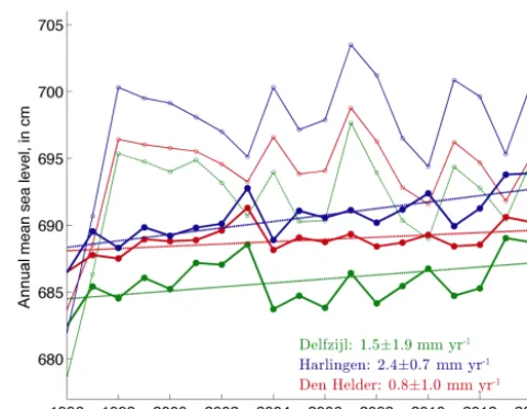
Figure 2.Annual mean sea level at three tide gauges in the Dutch Wadden Sea, during the past half century. The record of the last 20 years is indicated in thin solid lines. The 50-year trend (least squares fit) is plotted in thick solid lines and listed in the legend, together with the 95 % confidence interval.
In Fig. 2, we show the annual mean values of sea level for the period 1966–2015, for three tide gauges in the Dutch Wadden Sea. Trends, plotted in solid lines, are based on this 50-year period. We obtained the trends from a least squares fit (for a discussion on alternative methods, see Dangendorf et al., 2015). The 95 % confidence interval on the slope is indicated in the legend and is calculated by a standard sta-tistical method (Montgomery and Runger, 2003), namely as ±tα/2,n−2
√
SSE/(n−2)Sxx. Hereα=0.05 for a 95 % con-fidence interval, sample size is n,SSE is the error sum of squares SSE=P(yi− ˆyi)2, and Sxx=P(xi− ¯x)2, where (xi, yi) are the observations,x¯ is the mean of the setxi, and
ˆ
yi are the regression values;tis the two-tailedt value. However, time series of sea level may exhibit serial corre-lation, which reduces the effective sample size. We account for this effect by replacingnwith an effective sample sizen∗
in the calculation of the confidence interval, following a com-mon procedure (e.g., Santer et al., 2000). First, we calculate the lag-1 autocorrelation coefficient (r1) of the de-trended se-rieseyi=yi− ˆyi, i.e., the correlation between (ey1,· · ·,eyn−1) and (ey2,· · ·,eyn). The effective sample size then follows as n∗=n(1−r1)/(1+r1). For the three cases shown in Fig. 2,
the confidence interval is, on average, enlarged by a factor of 1.24 as a result of usingn∗instead ofn.
To test the robustness of the trends, we alternatively cal-culated them by using the Theil–Sen method (e.g., Sprent, 1993), which has the advantage of being less sensitive to out-liers than linear regression. The difference between the meth-ods was found to be slight: 0.1 mm yr−1at most. Hereafter, we opted for linear regression because the associated method of obtaining confidence intervals is more firmly established.
The trends differ between the stations but not beyond the margin of uncertainty, as indicated in the legend of Fig. 2.
Table 1.Trends in sea level rise and 95 % confidence intervals (all in mm yr−1) for annual and seasonal half-year means. (Derived from 100-year records, 1916–2015, supplied by Rijkswaterstaat and PSMSL.)
Station Annual mean Summer mean Winter mean
Delfzijl 1.95±0.31 1.65±0.24 2.28±0.50 Harlingen 1.27±0.32 0.88±0.29 1.69±0.49 Den Helder 1.59±0.30 1.34±0.26 1.87±0.44 IJmuiden 2.15±0.38 1.87±0.34 2.48±0.45 Hoek van Holland 2.36±0.30 2.13±0.25 2.64±0.42 Vlissingen 2.07±0.31 1.90±0.29 2.25±0.36
A longer record is needed to sufficiently reduce the con-fidence intervals and ascertain a difference in trends, as demonstrated by de Ronde et al. (2014) and seen in the re-sults from a 100-year record shown in Table 1.
Our focus in this paper is on the last 20 years, i.e., the pe-riod 1996–2015 (indicated in thin solid lines in Fig. 2). It is of great interest to know whether the trend from the past half century has continued during the last 2 decades, or whether there is an acceleration or deceleration in the rise. However, for the period 1996–2015, taken in isolation, the 95 % con-fidence interval is as large as±5.4 mm yr−1, the average for the six tide gauge stations marked in Fig. 1. This wide con-fidence interval precludes a meaningful estimate of a recent trend from these data. It is worthwhile pointing out that the effect of using the effective sample size is considerable: it almost doubles the confidence interval in comparison with one calculated by using simply the actual sample size, which would have produced±2.8 mm yr−1 (again the average for the six stations).
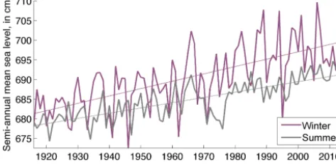
exam-Figure 3.Evolution of winter and summer half-year mean sea lev-els at Den Helder and corresponding trends from linear regression. See also Table 1 for the slope and confidence interval of the trends.
ple is Harlingen, where mean winter levels rose nearly twice as fast as mean summer levels; the distinction between the trends is statistically significant because the confidence in-tervals show no overlap. For the other stations, there is some overlap; yet, the fact that the sharper rise during the winter half-year occurs for all stations makes it plausible that the phenomenon is real. Its relevance extends to projections of risks of flooding, where trends of annual mean values have been the default reference. The distinction between half-year trends matters because severe storms (in northwest Europe) mostly occur in the winter half-year, when the background mean sea level is already higher than the annual mean and moreover has been rising more rapidly, as Table 1 suggests.
The trends based on annual mean values, also listed in Ta-ble 1, lie in-between those half-year trends and are in agree-ment with previously calculated trends by Wahl et al. (2013). Besides the problem of a difference in trend between sum-mer half-year and full years, the reduction in the confidence interval gained by selecting the summer half-year is actually modest (see Table 1). Hereafter, we therefore focus on annual mean values, i.e., derived from full-year data.
2.2 Wind record
We analyze records of wind data from Vlieland weather sta-tion (KNMI stasta-tion 242), which is located on a large sand flat. There are no obstacles in its immediate vicinity, and it lies well exposed to winds from all angles. The data are publicly available from a portal of the KNMI (Royal Netherlands Me-teorological Institute) at http://projects.knmi.nl/klimatologie/ uurgegevens. Records of wind speed and direction from KNMI weather stations span in some cases more than a cen-tury. However, from time to time, changes have occurred in the measurement techniques, which may have produced in-homogeneities in the time series. This involves, for instance, changes in the height or location of the instruments, a re-placement of instruments, changes in surrounding vegeta-tion or buildings, or changes in protocol, as documented by Verkaik (2001). Thus, the KNMI data come with the caveat
that the “series are not suitable for trend analysis”. For exam-ple, the Kooy/Den Helder weather station (used by de Ronde et al., 2014) has been subject to some relocations, which has impaired the homogeneity of the record. To avoid these problems, we restrict ourselves to data from the 20-year pe-riod 1996–2015 recorded by the automatic weather station on Vlieland, without apparent inhomogeneities (apart from a few gaps, discussed below).
Hourly values of wind speedW and directionDare used. They are defined as the mean speed and direction during the last 10 min interval of the preceding hour and are labeled with hourly interval indexi.
We divide the wind direction into eight sectors, la-beled with n=1, . . .,8, respectively as follows: northerly (N), northeasterly (NE), easterly (E), southeasterly (SE), southerly (S), southwesterly (SW), westerly (W), and north-westerly (NW). This is the direction fromwhich the wind blows.
To characterize the wind climate, we will use wind en-ergy, but other quantities could be used as well. Another nat-ural choice would be the wind stress. However, one then has to adopt a formulation for the drag coefficient in terms of wind strength, which should be valid for the entire range from breezes to hurricanes. A simple form of the drag co-efficient (e.g., Guan and Xie, 2004) would involve a linear dependence on wind speedW, implying a cubic power in the stress. By using energy, we get that power straight away without having to enter the uncertain territory of how to de-fine the drag coefficient. We carried out tests and found that the results are actually not very sensitive to the choice of the power. This agrees with the finding by Richter et al. (2012) that it is immaterial whether one uses wind speed or stress.
Hourly wind speed (as defined above) has a certain magni-tudeWn,i, with sectorial directionn. The kinetic energyEn of wind crossing a vertical plane area Acan be written as follows:
En,i = 1 2mn,iW
2 n,i=
1 2ρVn,iW
2 n,i=
1
2ρA1t W
3 n,i,
with massmand volumeV, which equals the areaAtimes the lengthW 1t (1t is the hourly interval, in seconds). We assumeρ, the density of air, to be constant (1.225 kg m−3, at sea level with temperature 15◦C); the areaAis taken to be 1 m2.
In a given year, the total number of data points, for all di-rections combined, is denoted byMa(this number may dif-fer between years because of leap years or occasional gaps in the data that arise when the wind direction is too variable and hence undefined). Thus, for a given sectorial directionn, the annual mean energy is
En=Ma−1 X
i
En,i= 1
2ρA1t M
−1 a
X
i
Wn,i3
=CMa−1X
i
Figure 4.Annual mean wind energy at Vlieland weather station, divided into eight sectorial directions. In(a)the average over the 20-year record (1996–2015), in black. The vertical line segments represent the standard deviations for each sector, as an indication of the typical interannual variability. Also shown are the averages of the summer half-year (in red) and winter half-year (in blue). In(b)the sectorial annual mean wind energy for all individual years. For clarity, the extreme years 1996 (dark blue) and 2015 (dark red) are highlighted with triangles alongside the bars.
with constantC=1
2ρA1t=2.2×10
3kg s m−1. We follow this procedure for all individual years. Wind energy will be expressed in megajoules (MJ).
The data from Vlieland weather station contain a few gaps (20–21 December 2002, 13–19 February 2008, and 2 July– 3 August 2015). They were filled in by substituting data from another weather station on a neighboring island (Ter-schelling Hoorn). The long-term mean energy levels are gen-erally lower there than at Vlieland because the station lies more sheltered, especially from northerly winds. However, for each individual wind sector the ratio is nearly constant over the years, so we can reliably fill in the missing data from Vlieland by using the data from Terschelling and ap-plying the correction factors to the individual sectors. One day in 2002, when neither station worked, missing data were filled in by linear interpolation.
2.3 Wind climate and interannual variability
Averaging over the full 20-year record (Fig. 4a), we find that the highest wind energy comes from the southwesterly and westerly directions. Together, they contain more energy than all other directions combined. The lowest energy comes from the northeasterly and southeasterly directions. We have com-pared this sectorial distribution with those from some other weather stations in the northeastern and southwestern cor-ners of the Netherlands (Huibertgat and Lichteiland Goeree, respectively); they confirm this pattern but appear less ex-posed to offshore winds than Vlieland weather station. In Fig. 4a, we also show the difference between winter and sum-mer half-years, again averaged over the 20-year record. For all major sectors, wind energy is substantially lower in sum-mer, most markedly so for southerly winds.
Focusing now on the interannual variability, we look at the sectorial distribution for all individual years from 1996 to 2015 (Fig. 4b). In terms of the absolute range of values at-tained, the interannual variability is largest for the southwest-erly direction. Alternatively, we can quantify the variability for each individual sector by calculating its relative standard deviation (i.e., the standard deviation divided by the mean, and expressed as a percentage). This gives 28 % (N), 34 % (NE), 49 % (E), 26 % (SE), 36 % (S), 25 % (SW), and 26 % (W), and 26 % (NW).
In contrast, the annual mean wind energy for all sectors combined, i.e., summed over the eight sectors, turns out to be fairly constant throughout the 20-year record (see Fig. 5). Its relative standard deviation is 13 %, which is much smaller than the value for any of the individual directions (listed above). Hence, it is not so much the total wind energy that varies between years but rather the share each of the sectors gets from this total.
As an aside, we note that the somewhat oscillating pattern in Fig. 5, with minima in 1997, 2003, and 2010, does not ap-pear to have any obvious connection with indices like ENSO or NAO.
3 Correlations
We first give a detailed overview of the results from the tide gauge at Den Helder before summarizing the results from the other stations.
3.1 Wind sectors and annual mean sea level
Figure 5.Annual mean wind energy summed over all eight sectors, at Vlieland weather station. The 20-year mean is indicated by the horizontal grey line.
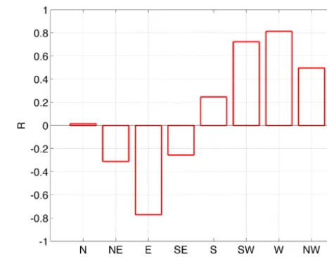
between the annual mean wind energy for each of the eight sectors and the annual mean sea level at Den Helder. The outcome is shown in Fig. 6. The high correlations for the easterly and westerly winds stand out, with correlation coef-ficientsR= −0.77 and+0.81, respectively. The negative co-efficient means that easterly winds lower the mean sea level, as they drain off water from the Wadden Sea into the North Sea. Westerly winds have the opposite effect, resulting in a positive correlation coefficient. This relationship was already observed on a much shorter timescale of one tidal period (Duran-Matute et al., 2016). Indeed, the mechanistic rela-tionship between wind and surges or depressions of sea level comes into play on the timescale of hours to days; models are well able to capture this (e.g., Zijl et al., 2013). On an annual timescale, the aggregate wind energy and mean sea level still show such a connection; the aggregate of the mechanistic ef-fects that actually occur on a much shorter timescale.
The predominant role of zonal winds at the Dutch coast agrees with recent results by Dangendorf et al. (2014) and Frederikse et al. (2016) for the North Sea area. They found a contrasting outcome at the British North Sea coast, where the role of the wind is much smaller and is surpassed by the inverted barometer effect.
Figure 6 is useful for providing a first impression, but the eight sectors cannot be regarded as independent. In a vecto-rial sense, after all, there are only two independent compo-nents in the wind direction.
3.2 Vectorial wind direction, air pressure, and annual mean sea level
To examine the vectorial (as opposed to sectorial) wind di-rection, we return to the original wind data and now decom-pose every hourly value ofDiinto west–east and south–north
Figure 6.Correlation coefficient R, based on a 20-year record, representing the correlation between annual mean sea level at Den Helder (Fig. 2) and annual aggregate wind energy for each of the eight sectors, calculated from the wind record at Vlieland weather station (Fig. 4b).
components, Di being the direction from which the wind blows. The angleDiis defined east of north.
We apply this decomposition of direction to the energy values and then sum, for every individual year, all west–east contributions and all south–north contributions:
EWE= −CMa−1 X
i
Wi3sin(Di),
ESN= −CMa−1 X
i
Wi3cos(Di). (2)
The minus signs on the right-hand side mean that winds from the west or south count as positive, and winds from the east or north as negative. (In the hypothetical case that there is as much energy in winds from the west as from the east, the result of the summation will be zero.) For proper comparison between years, we divide by the total annual number of data points, Ma.EWE andESN thus represent the annual mean vectorial components of the wind energy.
3.3 Simple correlation
oppo-Figure 7.Annual mean sea level versus the annual mean west–east energy component; the correlation isR=0.92. The least squares fit is shown as the grey line.
site case occurred in 2015 (red triangles in Fig. 4), which we correspondingly find farthest on the right in Fig. 7.
The grey line in Fig. 7 shows the least squares fit. Using this line and the values of the annual aggregate WE wind en-ergy, we can calculate a reconstructed annual mean sea level. The result is shown in Fig. 8, blue line. It lies close to the observed annual mean sea level (in black), which means that the WE wind already explains most of the interannual vari-ability.
For the other two tide gauge stations in the Dutch Wad-den Sea, we can follow the same procedure and find similar correlation coefficients: 0.90 (Harlingen) and 0.88 (Delfzijl). For the additional tide gauges shown in Fig. 1, the correlation decreases to 0.73 for Vlissingen, suggesting a weaker influ-ence by WE winds and a larger role for other factors, which will be confirmed below.
3.4 Multiple regression
We can improve on this result by also including the annual mean south–north component of wind energy as well as the annual mean atmospheric pressure, pann (in addition, one may include time, in years, as a fourth independent variable; we discuss this in Sect. 5.1). We deal with all three inde-pendent variables at once by using multiple regression (the backslash operator in MATLAB).
For Den Helder, the resulting reconstruction of annual mean sea level is shown as the red line in Fig. 8. Other stations can be treated in the same way; the collected re-sults are shown in Table 2. In all cases, the west–east wind energy coefficient is dominant and positive. The south– north wind energy carries a negative coefficient, implying that southerly (northerly) winds create a lowering (surge) in mean sea level. The inverted barometer effect is found to
Figure 8.Observed annual mean sea level at Den Helder is repli-cated in black from Fig. 2. The blue and red lines represent recon-structed annual mean sea levels based on atmospheric data. The blue line results from the annual mean west–east component of wind en-ergy combined with the least squares fit of Fig. 7. The red line uses a multiple regression involving both directions of the wind energy vector (i.e., west–east and south–north) as well as the annual mean atmospheric pressure at Vlieland weather station. The green dashed line is a reconstruction based on reanalysis data.
be 0.95 cm mbar−1 (on average), which is close to the the-oretical value of 1.0 cm mbar−1 (e.g., Pugh, 2004). Annual mean pressure at Vlieland weather station varies between 1013 and 1017 mbar; hence, this range accounts for an in-terannual variability in mean sea level of at most 4 cm.
The upshot is that we can construct an annual mean sea levelζcfrom the atmospheric data. Overall, this constructed level corresponds with the observed annual mean sea level to within the errors listed in Table 2. The constructed level is given by
ζc=C0+CWE×EWE+CSN×ESN+Cp×pann.
As constantsC0,CWE,CSN, andCp are known from mul-tiple regression, we can use meteorological dataEWE,ESN, andpann to estimate the mean sea level for any given year. It is important to realize that the constants depend on the lo-cation of the tide gauge, as indicated in Table 2. In particu-lar, the sensitivities on WE and SN winds vary spatially. An extreme case is Harlingen, with the highest factor for WE winds and the lowest for SN winds; the other extreme, Hoek van Holland and Vlissingen, have the lowest factor for WE winds and the highest for SN winds.
Table 2.Coefficients representing the effect of the wind climate and atmospheric pressure on annual mean sea level. Each is based on a combination of data from a tide gauge and Vlieland weather station. The root-mean-square error of the least squares fit is also listed. The trend with 95 % confidence interval is obtained from linear regression after correcting observed annual mean sea levels for meteorological effects. In brackets, we list the results from an extended multiple regression in which time is included to allow for a direct estimate of the trend; this is discussed in Sect. 5.1.
Coefficient Delfzijl Harlingen Den Helder IJmuiden Hoek van Holland Vlissingen
C0(103cm) 1.62 (1.59) 1.64 (1.60) 1.48 (1.47) 1.61 (1.60) 1.83 (1.81) 1.71 (1.67) CWE(cm MJ−1) 14.9 (14.2) 16.7 (15.5) 12.2 (11.7) 12.2 (12.0) 10.0 (9.28) 10.7 (9.57) CSN(cm MJ−1) −2.42 (−2.55) −1.76 (−1.97) −3.01 (−3.08) −3.98 (−4.02) −5.21 (−5.34) −7.27 (−7.47) Cp(cm mbar−1) −0.92 (−0.89) −0.94 (−0.90) −0.79 (−0.77) −0.90 (−0.90) −1.13 (−1.10) −1.01 (−0.97) RMS error (cm) 2.04 (1.85) 2.00 (1.24) 1.16 (1.05) 1.62 (1.64) 1.59 (1.27) 1.95 (1.34) Trend (mm yr−1) 1.5±1.9 (1.6) 2.4±0.7 (2.6) 0.8±1.0 (0.9) 0.4±1.7 (0.5) 1.5±0.9 (1.6) 2.2±1.0 (2.3)
Vlissingen, it would seem natural to take a more nearby weather station instead. However, it turns out that this makes the reconstruction worse. This may in part be due to the lesser quality of the data, but it also relates to the question of what spatial scale in the end determines the local annual mean sea level. In the case at hand, presumably, the crucial factor is how the wind in the central North Sea creates surges; for this, the Vlieland weather station is more indicative than other, more remote stations.
3.5 Corrected levels
Finally, we can correct for the atmospheric effects as quanti-fied in Table 2 by subtracting the atmospheric-induced vari-ations, contained in ζc, from the original observed annual mean sea level ζobs. The result is shown in Fig. 9 for the three tide gauge stations in the Wadden Sea. We arbitrarily introduced an offset, for which we choose the reference level corresponding with long-term mean atmospheric pressurep¯, i.e.,C0+Cpp¯.
Figure 9 demonstrates that the interannual variability is greatly reduced by the atmospheric correction. Using linear regression, we can calculate the trend of the corrected signal, along with the 95 % confidence interval on the slope; they are listed in the legend of Fig. 9 and in Table 2. For the six sta-tions depicted in Fig. 1, the mean 95 % confidence interval is ±1.2 mm yr−1, which is smaller by a factor of 4.5 compared to the interval derived from the original (i.e., uncorrected) 20-year data set, as discussed in Sect. 2.1. It is also interesting to note that the atmospheric correction reduces the difference between using the effective and the actual sample size; the latter gives a confidence interval of±1.1 mm yr−1. Without correction for atmospheric effects, the difference was much larger, as discussed in Sect. 2.1. This means that the atmo-spheric corrections reduce the serial correlation in the time series.
Whilst the confidence intervals are still too large to draw conclusions on a possible change of trend compared to the 50-year period, their reduction demonstrates that a correction for meteorological factors offers a substantial gain.
Figure 9.Annual mean sea level at three tide gauges in the Dutch Wadden Sea replicated in thin lines from Fig. 2 for the stations Delfzijl (green), Harlingen (blue), and Den Helder (red). Also shown is the result after correction for atmospheric effects (thick lines), together with fits from linear regression (dashed). The trend with 95 % confidence interval on the slope is listed in the legend for each case.
4 Regional variability
Figure 10.Annual mean sea level for the years 2009–2011: comparison between model results (asterisks) and observations (circles) for fourteen tide gauges in and around the Dutch Wadden Sea, whose positions are indicated in the map on the left.
Figure 11.Model result: the 3-year mean sea level for the years 2009–2011. Intertidal areas, which fall dry part of the time, are left out and rendered white.
Duran-Matute et al. (2014) and Gräwe et al. (2016). In this section we explore how well the model captures the inter-annual variability and we identify spatial patterns (the data are available at Gerkema and Duran-Matute, 2017). Data are used from the tide gauges shown in Fig. 10a. To facilitate comparison with the model, we will use the datum of NAP (Normaal Amsterdams Peil), which follows approximately the geoid, i.e., the equipotential of the gravity field. Water depth and bathymetry, both in observations and model, are taken with respect to this reference. In the model, however, the equipotential is represented by a plane surface.
Apart from an offset, the model captures the interannual variability well (Fig. 10b). The offset between modeled and observed values is for each station nearly constant through the years, but it differs between stations. On average, the off-set is 2.1 cm, which may be due to a slight imprecision in the open boundary conditions.
Both in observations and model results, it is remarkable how strong the spatial variability is in each year, with per-sistently higher levels around stations 7, 8, and 10. This is further highlighted in Fig. 11, a spatial plot of the 3-year
mean sea level for the period of the model run, 2009–2011. Clearly, stations 7, 8, and 10 form part of a wider area of higher mean sea levels. The location is consistent with our findings in Sect. 3.4 that the sensitivity of mean sea level to winds in the west–east direction is strongest at Harlingen (station 10), as represented by the coefficientCWEin Table 2. This points to the wind as being a principal factor in the spa-tial variability of annual mean sea level in Fig. 11. It is not that the wind itself would vary much over this small region but rather the local sensitivity of annual mean sea level to a given wind climate. In the case of this inter-tidal area, it is plausible that this spatial variation in sensitivity is mainly de-termined by the morphology of the basin. Due to the predom-inantly southwesterly/westerly winds (see Fig. 4a), a mean wind setup is created at eastward boundaries. Accordingly, the setup at watersheds is generally higher at the western side than at the eastern side. More evidence of the role of the wind in the spatial variability comes from the study by Duran-Matute et al. (2016), where on tidal timescales a qual-itatively similar spatial response was seen for (south)westerly winds.
Besides the wind, freshwater sources may play a role. Al-though we found no significant improvement in the results by adding an overall measure of freshwater discharge (as dis-cussed below, in Sect. 5.4), it is conceivable that there are local effects, in particular in this case, since stations 7 and 8 lie at sluices. Future model studies (e.g., with and without freshwater discharge) could shed light on the significance of a local discharge.
5 Discussion
5.1 Optimizing multiple regression
In the previous section, we presented a way to correct for at-mospheric pressure and wind effects, resulting in a corrected signal whose trend we can determine. Alternatively, we can obtain the trend directly from multiple regression by includ-ing time (in years) as an additional independent variable, along with the wind components and pressure. This results in the values listed in brackets in Table 2. They are in fact close to those already obtained; for deriving trends, it is im-material which procedure is followed. On the other hand, the root-mean-square errors are generally reduced by including the trend in the multiple regression, especially in the case of Harlingen, which is not surprising since the trend is strongest there.
5.2 Possible asymmetries in the wind effect
In the analysis in this paper, we considered the vectorial sum of the wind energy as an explanatory factor for annual mean sea level. This means that energy from westerly and east-erly winds are lumped together (i.e., subtracted) as if they carry equal weight. However, it is important to keep in mind that this serves only as a first-order approach, since in real-ity the relationship will be more asymmetric. In the case of the Dutch Wadden Sea, an easterly wind has less fetch and can drain off only a limited amount of water (because of the shallowness of the basin) compared to westerly winds, which have a longer fetch and carry a larger potential for heighten-ing sea level, with waters comheighten-ing from the large reservoir of the North Sea. A weighting factor is thus likely to be in-volved, but this will not be examined further in this paper.
5.3 Effect of extreme surges on annual mean sea level
An important question is whether the annual mean sea level is mainly controlled by a few extreme surges during heavy storms, or rather reflects the aggregate of all the contribu-tions of the various condicontribu-tions throughout the year. This de-termines whether storm surges ride, as it were, on top of a background mean sea level or, instead, they shape that very level.
To answer this question, we consider a 20-year record of the tide gauge at Den Helder (period 1996–2015, as else-where in this paper), with data at 10 min intervals (using pub-licly available data from the Dutch governmental agency Ri-jkswaterstaat). As a reference we take the datum NAP. Dur-ing this period, mean high tide was +59 cm, and mean low tide−80 cm. The highest level in this record is+271 cm.
We here define “extreme surges” as levels exceeding mean high tide plus 100 cm, i.e., higher than+159 cm. With this criterion, we place the bar rather low for an event to be counted as “extreme” (this level falls in the official cate-gory “low storm surge”). Nevertheless, the combined effect
of all these “extreme” events contributes on average still only +0.34 cm to the annual mean sea level, and in none of the years more than+1.0 cm.
Since the interannual variability of annual mean sea level lies rather on the order of several centimeters up to a few decimeters (see Fig. 2), it is clear that these variations cannot be ascribed to the incidence of extreme events; instead, they must be primarily controlled by the more typical conditions that prevail in a certain year. Although intense, the extreme events last too short to leave a fingerprint on the annual mean level.
Conversely, however, there are indications that changes in mean sea level can result in a change in extremes (both in terms of level and frequency), as pointed out by Woodworth et al. (2011).
5.4 Other effects
Another possible cause of variability is the 18.6-year lu-nar nodal cycle. This cycle has two distinct effects. On the one hand, it modulates the amplitude (and phase) of the lu-nar constituents, notably the principal semidiurnal lulu-nar con-stituent M2 and lunar declinational diurnal concon-stituents K1 and O1. This has a very significant effect on the tidal range and on the diurnal inequality, but it leaves the annual mean sea level unaffected since high waters are as much higher as low waters are lower, canceling out in the mean. On the other hand, there is a small long-period nodal constituent N, which has no effect on the tidal range but does have a sig-nature in annual mean sea level. Exactly how important this effect is still appears to be a matter of debate. According to Pugh (2004), the amplitude is about 4.4 mm around Europe. Baart et al. (2012) included a nodal oscillation in their fit to annual mean sea level at the Dutch coast (combining six tide gauge stations). They find an amplitude of 1.2 cm, with the maximum occurring in February 2005. However, our results, after correction for atmospheric effects show no maximum at that time. Moreover, as Woodworth (2012) emphasized, the 18.6-year cycle cannot really be distinguished from decadal variability in short records (like ours), while the cycle will hardly affect trends in long ones; hence Woodworth paren-thetically suggests “just forgetting it for many midlatitude coastlines” – which is what we have done in this paper.
On the decadal timescale, variability in land water storage (due to ENSO) has been found to have a fingerprint in annual mean sea level, with a lowering during La Niña events, such as in 2007–2009 (Woodworth et al., 2011). This, however, is not clearly visible in our corrected annual mean sea levels (Fig. 9).
be-fore splitting into different branches using publicly available data from the Dutch governmental agency Rijkswaterstaat) gave no substantial improvement in the multiple regression analysis, confirming a similar conclusion by de Ronde et al. (2014).
5.5 Comparison with reanalysis data
In this study, we have used an observed meteorological record from Vlieland weather station (Fig. 1). An alterna-tive is to use reanalysis data. Here we compare the two. We use ECMWF ERA-Interim reanalysis data (Dee et al., 2011), which include wind and atmospheric pressure at 6 h inter-vals. We examine the same time span as in previous sections, 1996–2015. From a grid corresponding to the effective model resolution, we select a point that lies in the North Sea; the lo-cation is indicated by a star in Fig. 1 (a more southern point, which is strictly closer to Vlieland, actually produces a worse result because of its being sheltered by the coast on the east). The overall 20-year levels of wind energy give a qualita-tively similar distribution over the sectors as in Fig. 4a for the observed record. For individual sectors, the reanalysis data differ as follows:−12 % (N),+24 % (NE),−2 % (E), +43 % (SE),+1 % (S),+7 % (SW),−2 % (W), and+36 % (NW). For the dominant directions, SW and W, the difference is relatively small.
All the steps from previous sections can be repeated, but now using the reanalysis data, leading to another reconstruc-tion of annual mean sea level, shown as the green line in Fig. 8. The reconstruction is slightly less good than the one based on the observed record (shown in red). For the reanal-ysis data, we find a root-mean-square error of 1.51, against 1.16 when using the observed record.
6 Conclusions
We find that at the Dutch coast, southwesterly winds are dominant in the wind climate (Fig. 4a), but west–east direc-tions stand out as having the highest correlation with annual mean sea level (Fig. 6). For different stations in the Dutch Wadden Sea and along the coast, we find a qualitatively sim-ilar pattern, although the precise values of the correlations vary. The interannual variability of mean sea level can al-ready be largely explained by the west–east component of the net wind energy vector, with some further improvement if one also includes the south–north component and annual mean atmospheric pressure. Knowledge of these local corre-lations can then be used to correct annual mean sea for these atmospheric effects and thereby reduce the margin of error in the trend.
We showed that a modest reduction in the margin of er-ror of trends in mean sea level rise can be obtained by se-lecting the summer half-year instead of the full year because of lower wind-induced variability. However, these summer trends are not representative of the annual mean trends, in
agreement with earlier findings by Dangendorf et al. (2013). For all stations studied here, we find from 100-year long records a steeper rise in the winter half-year than in sum-mer half-year values of mean sea level. This is an apparently overlooked but relevant feature in view of coastal protection, since severe storms are more common during the winter half-year.
This study implies that climatic changes in the dominant wind direction or in the strength of winds from any specific sector may affect the annual mean sea level quite signifi-cantly. For the Netherlands, no trend in wind strength has been found for reconstructed wind fields in the 20th century (calculated as geostrophic winds from atmospheric pressure records, KNMI, 1999), but to date, no study seems to have been carried out for possible trends in individual wind sec-tors. Climate studies tend to focus on extreme events such as the frequency of severe storms and maximum wind speed (see, e.g., de Winter et al., 2013) rather than on the annual mean wind energy for different wind sectors.
Such changes in wind climate may affect locations differ-ently; as this study shows, some places have a higher corre-lation with winds in the west–east (or south–north) direction than others (see Table 2). This sensitivity to wind direction has a regional variability, as is suggested by the model result in Fig. 11 and supported on shorter timescales by the mod-eling study by Duran-Matute et al. (2016). Even on a small scale like the Dutch Wadden Sea, there is a spatial variability in the response of the annual mean sea level to changes in the wind climate.
Data availability. Publicly available wind and atmospheric pres-sure records were used from the KNMI (Royal Netherlands Me-teorological Institute) for the weather stations Vlieland (no. 242) and Hoorn Terschelling (no. 251), which the KNMI provides at http://projects.knmi.nl/klimatologie/uurgegevens.
Publicly available monthly mean sea level data for tide gauge stations at the Dutch coast were used, which the PSMSL (Permanent Service for Mean Sea Level) provides at www.psmsl.org.
Sea level data at 10 min resolution of the tide gauge at Den Helder (1996–2015) are publicly available and provided by the Dutch governmental agency Rijkswaterstaat via the portal http: //live.waterbase.nl. Here, the data of the Rhine discharge at Lobith are also provided.
Publicly available atmospheric reanalysis data were used (ERA-Interim), which the ECMWF provides via the portal http://apps. ecmwf.int/datasets/.
The model data for mean sea level in the Dutch Wad-den Sea (2009–2011) used in Figs. 10 and 11 can be found at https://doi.org/10.4121/uuid:115ef6c5-8c58-4905-91f5-537985fb3b6f (Gerkema and Duran-Matute, 2017).
Acknowledgements. We thank Thomas Frederikse (TU Delft) and Vincent Vuik (HKV) for bringing several relevant papers and reports to our attention, as well as Andreas Sterl (KNMI) for advice and help on the usage of reanalysis data.
Edited by: Yun Liu
Reviewed by: three anonymous referees
References
Baart, F., van Gelder, P. H. A. J. M., de Ronde, J., van Koningsveld, M., and Wouters, B.: The Effect of the 18.6-Year Lunar Nodal Cycle on Regional Sea-Level Rise Estimates, J. Coastal Res., 28, 511–516, 2012.
Baart, F., Leander, R., de Ronde, J. G., de Vries, H., Vuik, V., and Nicolai, R.: Zeespiegelmonitor 2014, Rekenmethode voor huidige en toekomstige zeespiegelstijging, Deltares Report 1209426-000-VEB-0011, 2014 (in Dutch).
Dangendorf, S., Mudersbach, C., Wahl, T., and Jensen, J.: Characteristics of intra-, inter-annual and decadal sea-level variability and the role of meteorological forcing: the long record of Cuxhaven, Ocean Dynam., 63, 209–224, https://doi.org/10.1007/s10236-013-0598-0, 2013.
Dangendorf, S., Calafat, F. M., Arns, A., Wahl, T., Haigh, I. D., and Jensen, J.: Mean sea level variability in the North Sea: Processes and implications, J. Geophys. Res., 119, 6820–6841, https://doi.org/10.1002/2014JC009901, 2014.
Dangendorf, S., Marcos, M., Müller, A., Zorita, E., Riva, R., Berk, K., and Jensen, J.: Detecting anthropogenic footprints in sea level rise, Nat. Commun., 6, 7849, https://doi.org/10.1038/ncomms8849, 2015.
de Ronde, J. G., Baart, F., Katsman, C. A., and Vuik, V.: Zeespiegel-monitor, Deltares report 1208712-000-ZKS-0010, 2014 (in Dutch).
de Winter, R. C., Sterl, A., and Ruessink, B. G.: Wind extremes in the North Sea Basin under climate change: An ensemble study of 12 CMIP5 GCMs, J. Geophys. Res.-Atmos., 118, 1601–1612, https://doi.org/10.1002/jgrd.50147, 2013.
Dee, D. P., Uppala, S. M., Simmons, A. J., Berrisford, P., Poli, P., Kobayashi, S., Andrae, U., Balmaseda, M. A., Balsamo, G., Bauer, P., Bechtold, P., Beljaars, A. C. M., van de Berg, L., Bid-lot, J., Bormann, N., Delsol, C., Dragani, R., Fuentes, M., Geer, A. J., Haimberger, L., Healy, S. B., Hersbach, H., Hólm, E. V., Isaksen, L., Kållberg, P., Köhler, M., Matricardi, M., McNally, A. P., Monge-Sanz, B. M., Morcrette, J.-J., Park, B.-K., Peubey, C., de Rosnay, P., Tavolato, C., Thépaut J.-N., and Vitart, F.: The ERA-Interim reanalysis: configuration and performance of the data assimilation system, Q. J. Roy. Meteor. Soc., 137, 553–597, https://doi.org/10.1002/qj.828, 2011.
Douglas, B. C.: Global sea level rise, J. Geophys. Res., 96, 6981– 6992, 1991.
Duran-Matute, M., Gerkema, T., de Boer, G. J., Nauw, J. J., and Gräwe, U.: Residual circulation and freshwater transport in the Dutch Wadden Sea: a numerical modelling study, Ocean Sci., 10, 611–632, https://doi.org/10.5194/os-10-611-2014, 2014. Duran-Matute, M., Gerkema, T., and Sassi, M. G.:
Quantify-ing the residual volume transport through a multiple-inlet sys-tem in response to wind forcing: The case of the
west-ern Dutch Wadden Sea, J. Geophys. Res., 121, 8888–8903, https://doi.org/10.1002/2016JC011807, 2016.
FitzGerald, D. M., Fenster, M. S., Argow, B. A., and Buynevich, I. V.: Coastal Impacts Due to Sea-Level Rise, Annu. Rev. Earth Planet. Sci, 36, 601–647, https://doi.org/10.1146/annurev.earth.35.031306.140139, 2008. Frederikse, T., Riva, R., Slobbe, C., Broerse, T., and Verlaan,
M.: Estimating decadal variability in sea level from tide gauge records: An application to the North Sea, J. Geophys. Res., 121, 1529–1545, https://doi.org/10.1002/2015JC011174, 2016. Gerkema, T. and Duran-Matute, M.: Annual mean
sea-level in the Dutch Wadden Sea 2009–2011, https://doi.org/10.4121/uuid:115ef6c5-8c58-4905-91f5-537985fb3b6f, 2017.
Gräwe, U., Flöser, G., Gerkema, T., Duran-Matute, M., Badewien, T., Schulz, E., and Burchard, H.: A numerical model for the entire Wadden Sea: skill assessment and analy-sis of hydrodynamics, J. Geophys. Res., 121, 5231–5251, https://doi.org/10.1002/2016JC011655, 2016.
Guan, C. and Xie, L.: On the Linear Parameterization of Drag Co-efficient over Sea Surface, J. Phys. Oceanogr., 34, 2847–2851, 2004.
KNMI: De toestand van het klimaat in Nederland 1999 (The state of the climate in the Netherlands), report Koninlijk Nederlands Meteorologisch Instituut, 1999 (in Dutch).
Lee, T. and McPhaden, M. J.: Decadal phase change in large-scale sea level and winds in the Indo-Pacific region at the end of the 20th century, Geophys. Res. Lett., 35, L01605, https://doi.org/10.1029/2007GL032419, 2008.
Merrifield, M. A. and Maltrud, M. E.: Regional sea level trends due to a Pacific trade wind intensification, Geophys. Res. Lett., 38, L21605, https://doi.org/10.1029/2011GL049576, 2011. Montgomery, D. and Runger, G.: Applied statistics and probability
for enigineers, Wiley, 3rd edn., 2003.
Pugh, D. T.: Changing sea levels: effects of tides, weather and cli-mate, Cambridge University Press, 2004.
Richter, K., Nilsen, J. E. O., and Drange, H.: Contri-butions to sea level variability along the Norwegian coast for 1960–2010, J. Geophys. Res., 117, C05038, https://doi.org/10.1029/2011JC007826, 2012.
Santer, B. D., Wigley, T. M. L., Boyle, J. S., Gaffen, D. J., Hnilo, J. J., Nychka, D., Parker, D. E., and Taylor, K. E.: Statistical sig-nificance of trends and trend differences in layer-average atmo-spheric temperature time series, J. Geophys. Res., 105, 7337– 7356, 2000.
Sprent, P.: Applied nonparametric statistical methods, Chapman & Hall, 2nd edn., 1993.
Stammer, D., Cazenave, A., Ponte, R. M., and Tamisiea, M. E.: Causes of contemporary regional sea level changes, Annu. Rev. Mar. Sci., 5, 21–46, https://doi.org/10.1146/annurev-marine-121211-172406, 2013.
Verkaik, J. W.: Documentatie windmetingen in Nederland (Docu-mentation of wind records in the Netherlands), report KNMI, 2001 (in Dutch).
Woodworth, P. L.: A Note on the Nodal Tide in Sea Level Records, J. Coastal Res., 28, 316–323, 2012.
Woodworth, P. L. and Player, R.: The Permanent Service for Mean Sea Level: An update to the 21st century, J. Coastal Res., 19, 287–295, 2003.
Woodworth, P. L., Gehrels, W. R., and Nerem, R.: Nineteenth and twentieth century changes in sea level, Oceanography, 24, 80–93, https://doi.org/10.5670/oceanog.2011.29, 2011.
Zervas, C.: Sea level variations of the United States 1854–2006, NOAA Technical Report NOS CO-OPS 053, 2009.