www.nonlin-processes-geophys.net/22/65/2015/ doi:10.5194/npg-22-65-2015
© Author(s) 2015. CC Attribution 3.0 License.
Fluctuations in a quasi-stationary shallow cumulus cloud ensemble
M. Sakradzija1,2, A. Seifert3, and T. Heus1,4
1Max Planck Institute for Meteorology, Hamburg, Germany
2International Max Planck Research School on Earth System Modelling (IMPRS-ESM), Hamburg, Germany 3Hans-Ertel Centre for Weather Research, Deutscher Wetterdienst, Hamburg, Germany
4Institute for Geophysics and Meteorology, University of Cologne, Cologne, Germany Correspondence to: M. Sakradzija (mirjana.sakradzija@mpimet.mpg.de)
Received: 21 May 2014 – Published in Nonlin. Processes Geophys. Discuss.: 4 August 2014 Revised: 9 December 2014 – Accepted: 19 December 2014 – Published: 28 January 2015
Abstract. We propose an approach to stochastic parameteri-sation of shallow cumulus clouds to represent the convective variability and its dependence on the model resolution. To collect information about the individual cloud lifecycles and the cloud ensemble as a whole, we employ a large eddy simu-lation (LES) model and a cloud tracking algorithm, followed by conditional sampling of clouds at the cloud-base level. In the case of a shallow cumulus ensemble, the cloud-base mass flux distribution is bimodal, due to the different shal-low cloud subtypes, active and passive clouds. Each distribu-tion mode can be approximated using a Weibull distribudistribu-tion, which is a generalisation of exponential distribution by ac-counting for the change in distribution shape due to the diver-sity of cloud lifecycles. The exponential distribution of cloud mass flux previously suggested for deep convection parame-terisation is a special case of the Weibull distribution, which opens a way towards unification of the statistical convective ensemble formalism of shallow and deep cumulus clouds.
Based on the empirical and theoretical findings, a stochas-tic model has been developed to simulate a shallow convec-tive cloud ensemble. It is formulated as a compound ran-dom process, with the number of convective elements drawn from a Poisson distribution, and the cloud mass flux sam-pled from a mixed Weibull distribution. Convective memory is accounted for through the explicit cloud lifecycles, mak-ing the model formulation consistent with the choice of the Weibull cloud mass flux distribution function. The memory of individual shallow clouds is required to capture the cor-rect convective variability. The resulting distribution of the subgrid convective states in the considered shallow cumulus case is scale-adaptive – the smaller the grid size, the broader the distribution.
1 Introduction
To set a path towards the development of a stochastic shallow-cloud parameterisation for numerical atmospheric models, we study how the unresolved convective processes relate to the resolved grid-scale variables in an ensemble of shallow cumulus clouds. According to a conventional deter-ministic approach to cloud parameterisation, the outcome of shallow cumulus processes within a grid box of a numerical model is represented as an average over the cloud ensemble or as a bulk effect. However, different microscopic configu-rations of a convective cloud ensemble can lead to the same average outcome on the macroscopic grid scale (Plant and Craig, 2008). If a one-to-one relation between the subgrid and grid scales is assumed, the spatial and temporal variabil-ity of convection that is observed in nature and in the cloud-resolving simulations will not be represented in atmospheric models. At the same time, the improvement in parameterisa-tion should address the dependence of the sub to grid-scale relation on the model resolution and physics time step (e.g. Jung and Arakawa, 2004). This is especially important on the meso-γ atmospheric scales, since moist convection and rain formation are recognised as the most uncertain pro-cesses acting on these scales and the core reason for the short mesoscale predictability limit (e.g. Tan et al., 2004; Zhang et al., 2003, 2006; Hohenegger et al., 2006).
Commonly used tools to study convective cloud processes at a high temporal and spatial resolution in order to develop parameterisations are the cloud resolving models (CRMs). To represent deep convective clouds explicitly, CRMs are used at the grid scale of 1 km order of magnitude, while shal-low convective clouds become explicitly resolved at a grid scale of O (10–100 m), which is the size of the largest
energy-producing eddies in the turbulent boundary layer, hence the name large eddy simulation (LES). To formulate the effects of clouds on their environment across the differ-ent scales of atmospheric flow, a technique of coarse graining can be applied to the CRM and LES fields (see, for example, Shutts and Palmer, 2007, Sect. 3). In this way, a relation be-tween the subgrid convection and the resolved flow can be emulated to reveal the properties and components of the pa-rameterisation and to reflect its dependence on the model grid resolution.
From the previous studies of deep convective cloud fields using CRMs and the coarse-graining methods, it is known that the subgrid- to grid-scale relation is neither fully deter-ministic nor diagnostic, which suggests that stochastic and memory components should be included in a parameterisa-tion. These components are sensitive to the spatial and tem-poral scales of a numerical model. As the horizontal reso-lution of a model gets higher, the stochastic component of the subgrid- to grid-scale relation becomes more pronounced (Xu et al., 1992; Shutts and Palmer, 2007; Jones and Randall, 2011). At the same time, an increase in horizontal resolu-tion implies a shorter model time step and, as a consequence, a larger impact of the memory component on parameterisa-tion. In this case, changes in the resolved flow take place on a timescale close to or less than the convective response timescale, and the convective cloud system exhibits a non-diagnostic behaviour (e.g. Pan and Randall, 1998; Jones and Randall, 2011). Along with the effects of time lag in the convective response, memory of convection also comprises a feedback process by which the past interactions between convective elements and thermodynamics fields on the near-cloud scale modify convection at the current time (Davies et al., 2013). Furthermore, a delay in the convective response becomes longer with the emergence of mesoscale cloud or-ganisation (Xu et al., 1992), and can be interpreted as an ad-ditional convective memory effect (Bengtsson et al., 2013).
A behaviour of the subgrid- to grid-scale relation similar to the behaviour of deep convection, but on the smaller spatial scales, can be confirmed in LES studies of shallow convec-tion. The stochastic effects in a coarse-grained shallow con-vective cloud ensemble become dominant on the scales close to 10 km and less (see Fig. 2 in Dorrestijn et al., 2013). We will refer to these spatial scales as the “stochastic” scales for the shallow convective ensemble.
Parameterisation schemes developed specifically for shal-low convection are in most cases based on the mass flux concept (Bechtold et al., 2001; von Salzen and McFarlane, 2002; Deng et al., 2003; Bretherton et al., 2004; Neggers, 2009). In a mass flux scheme, clouds within a model grid box are parameterised as a single bulk updraft or as a spec-trum of cloud updrafts via a simple entraining–detraining plume model, and the vertical transport is determined by the upward mass flux through the cloud base. Estimation of the bulk or ensemble average cloud-base mass flux is a part of the model closure and is based on some form of
the quasi-equilibrium assumption (Arakawa and Schubert, 1974). According to the quasi-equilibrium assumption, in a slowly varying large-scale environment, the subgrid con-vective ensemble is under control of the large-scale forcing with a statistical balance fulfilled between the unresolved and resolved processes. However, at the stochastic scales, the quasi-equilibrium assumption is no longer valid. The model grid box is not large enough to contain a robust statistical sample of shallow clouds and the timescale of parameterised processes can not be separated from the timescale of the re-solved processes. This suggests that a stochastic and non-diagnostic approach to parameterisation is necessary not only for representing the small-scale variability of convection, but also for representing the cloud field adequately by provid-ing a way to make the parameterisation scale-adaptive, and to avoid the scale-separation problem.
Increasing horizontal resolution of atmospheric models is also strongly connected to the mesoscale predictability limit, which is reached faster on the smaller scales of the resolved motion (Lorenz, 1969). The reason for a shorter predictabil-ity time on the smaller spatial scales comes from the faster error growth on these scales due to moist convection (Zhang et al., 2003, 2006). In the simulations with the grid resolution of the order of 1 km, the small-scale initial errors spread fast throughout the domain and exponentially amplify over the regions with the convective instability (Hohenegger et al., 2006). Due to non-linear interactions, initial uncertainties propagate upscale in a process known as the “inverse er-ror cascade” and degrade the forecast quality on the larger scales (Lorenz, 1969; Leith, 1971). Here the stochastic term of a parameterisation plays a role in representing the subgrid fluctuations that, due to the non-linearity of the process, lead to the error growth and upscale error propagation. Thus, the stochastic term provides a way to quantify the uncertainties coming from the formulation of the subgrid cloud processes and is necessary to improve the ensemble spread in the en-semble prediction systems – EPS (see the review of Palmer et al., 2005).
Recently, EPS have been developed for the limited area models at the convection-permitting grid resolution to ad-dress the sensitive dependence on initial conditions (e.g. Kong et al., 2007; Gebhardt et al., 2008; Clark et al., 2009; Migliorini et al., 2011). The main goal of this new field of research is the improvement of the quantitative precipitation forecasts and the forecasts of convective and storm events. In the convection-permitting models, deep convective clouds are explicitly represented on the grid scale, while the plan-etary boundary layer (PBL) convection and shallow clouds are still subgrid processes and have to be parameterised. Nevertheless, the introduction of the stochastic physics into the convection-permitting EPS has been limited so far. The stochastically perturbed parameterisation tendencies (SPPT) scheme of Buizza et al. (1999) is adapted and applied in a short-range convection-permitting EPS by Bouttier et al. (2012) to improve the ensemble reliability and the ensemble
spread–error relationship. Another example is the recent work of Baker et al. (2014), where another similar method of parameter perturbation of the model physics tendencies called the random parameters (RP) scheme (Bowler et al., 2008) is modified and applied to a convection-permitting EPS. Both of these approaches are rather pragmatic and gen-eral in perturbing the physical tendencies in a model. The ef-fect of stochastic schemes specifically developed for the shal-low clouds and based on the underlying physical processes has not been investigated so far, mainly because stochastic schemes for shallow clouds have not been formulated until recently. One example is the scheme developed for stochastic parameterisation of convective transport by shallow cumulus convection (Dorrestijn et al., 2013), based on LES studies of non-precipitating shallow convection over the ocean. In this scheme, the pairs of turbulent heat and moisture fluxes are randomly selected as corresponding to different states of a data-inferred conditional Markov chain (CMC). In another approach, two stochastic processes are implemented in the eddy-diffusivity mass-flux (EDMF) scheme (Siebesma et al., 2007; Neggers, 2009), the Monte Carlo sampling of the con-vective plumes and the stochastic lateral entrainment (Sušelj et al., 2013).
The goal of our study is to formulate a shallow convective parameterisation that encompasses the stochastic and mem-ory effects of convection, using the theoretical and empiri-cal findings about the cloud ensemble. We study a shallow convective-cloud case (Rain in Cumulus over the Ocean – RICO) using large eddy simulation (LES). RICO is a pre-cipitating quasi-stationary shallow convective case that also shows some mesoscale organisation. We coarse grain the cloud ensemble to study the subgrid- to grid-scale relation and its dependence on the horizontal resolution. The vari-ability of shallow convection and its scaling with the hori-zontal resolution is then quantified. Individual cloud lifecy-cles and the role of the diversity of cloud lifetimes are ex-amined employing the cloud tracking routine of Heus and Seifert (2013). This numerical study gives a path to apply the theory of fluctuations in an equilibrium convective ensemble of Craig and Cohen (2006b) to a shallow convective case.
In the following, we propose a generalisation of the the-ory of fluctuations in a convective ensemble by including the system memory and by considering the impact of the diver-sity in cloud lifecycles on the cloud-base mass flux distribu-tion shape. This provides a stochastic and memory term in the subgrid- to grid-scale relation, and a deterministic com-ponent is also retained in adequate proportion, depending on the grid scale. This combined empirical–theoretical concept is then structured in a stochastic stand-alone model of a shal-low cumulus ensemble, similar to the approach of Plant and Craig (2008) for deep convection, referred to as PC-2008 in the following text. A spectral representation of the cloud field with the cloud lifecycles modelled explicitly introduces the memory of individual clouds and opens the way to esti-mating the impact of this memory on the variability of
con-vection. Sensitivity tests of the gradual generalisation of the convective-fluctuation theory provide a definition of a con-sistent and least complex model formulation.
Large eddy simulation and the cloud tracking algorithm necessary for the analysis are described in Sect. 2. Physical and statistical properties of a cloud ensemble are described here and the cloud mass flux distribution is analysed. A stand-alone stochastic model is constructed based on em-pirical and theoretical findings and the model formulation is derived for the different levels of system generalisation (Sect. 3). Different formulations of the stochastic model are discussed, and tested against LES results, to decide on min-imal and consistent representation of all relevant features of subgrid convection and its variability (Sect. 4).
2 Shallow cumulus ensemble statistics
To develop a stochastic parameterisation for shallow cu-muli that includes convective memory in its formulation, a detailed description of the cloud ensemble and the pro-cesses acting on the scale of an individual cloud is necessary. A large eddy simulation as a cloud-resolving model suffices for the detailed description of the shallow cumuli field in a large horizontal area, while the cloud tracking as a post-processing routine collects the information about every sim-ulated cloud during its lifetime.
2.1 Large eddy simulations and cloud tracking
We use the UCLA-LES (University of California, Los Ange-les – Large Eddy Simulation) model, a version from Stevens (2010), to simulate shallow convection. The dynamical core of the LES model is based on the Ogura–Phillips anelas-tic equations, discretised over the doubly periodic uniform Arakawa C-grid (Stevens et al., 1999, 2005). The set of anelastic equations is solved for the prognostic variables: ve-locity components(u, v, w), total water mixing ratiort, liq-uid water potential temperatureθl, number ratio of rainwa-terNr and mass mixing ratio of rainwaterrr. The time in-tegration is solved using a third-order Runge–Kutta numer-ical method. A directionally split monotone upwind scheme is used for the advection of scalars, and directionally split fourth-order centered differences are used for the momen-tum advection. The subgrid fluxes are modelled by the Smagorinsky–Lilly scheme, and the warm-rain scheme of Seifert and Beheng (2001) is used for the cloud microphysics as described in Stevens and Seifert (2008).
In this study, the LES model is set up to simulate the GCSS (GEWEX Cloud Systems Studies) RICO shallow cu-mulus case, as in van Zanten et al. (2011). The RICO case is based on the Rain In Cumulus over the Ocean field study (Rauber et al., 2007). It represents the average conditions during an undisturbed period from 16 December 2004 to 8 January 2005 in the trade-wind region over the western
Atlantic. The focus of this field study was on the processes related to the rain formation in shallow cumuli and on how the rain modifies the individual cloud and the cloud ensemble statistics.
The standard RICO-GCSS case was simulated over a large domain of around 50 km×50 km, with the horizontal grid spacing of 25 m and vertical resolution of 25 m up to 4 km in height. In such a large domain and on a high-resolution grid, a cloud field can evolve into an organised mesoscale convec-tive system, forming clusters and line-like structures (Seifert and Heus, 2013). This transition to an organised cloud field depends mostly on precipitation rate and, for the RICO-GCSS simulation, the first organised cloud clusters develop around the twelfth hour of the simulation (Fig. 1d). In the RICO-140 case, which has a doubled cloud droplet number density, Nc=140 cm−3, and is virtually non-precipitating, the cloud field remains quasi-random, but the individual clouds grow in size throughout the simulation time (Fig. 1a, c, e and g). The convective variability in an organised case is, of course, very different from the variability of a quasi-random cloud field. This is discussed in more detail later in Sect. 4.2, where we discuss RICO-GCSS and RICO-140 to quantify the effects of organisation, but for most of the anal-ysis we focus on the simple case of the RICO-140 with a quasi-random cloud field.
The cloud tracking algorithm developed by Heus and Seifert (2013) is used as a post-processing tool for the LES simulation results. The tracking is based on the verti-cally integrated liquid water content, namely the liquid water path. The clouds are projected onto a two-dimensional plane and are identified as consisting of the adjacent points with the liquid water path exceeding a chosen threshold value. Cloud merging and splitting is done in two directions: for-ward and backfor-ward in time. Along with the projected cloud area, cloud buoyant cores, sub-cloud thermals and rain are tracked during the simulation, with the links among them re-tained. The choice of the two-dimensional tracking of the projected clouds came from the limitations imposed by the computational expenses and the large memory resources that are required. For more details and validation of the tracking method, see Heus and Seifert (2013).
To develop a cloud parameterisation based on the mass flux concept, the cloud mass flux has to be estimated at the cloud-base level. For the RICO case, we choose the level at 700 m, which is the first or second height level above the cloud base during most of the simulation time. Thus, it is necessary to identify the area that every cloud occupies at the 700 m level. Because the liquid water path threshold of 5 g m−2 is taken as a definition of a cloudy column in the cloud tracking algorithm and the clouds are projected onto a two-dimensional surface, we check what the error is intro-duced by the tracking regarding the domain average cloud variables at the 700 m height. We define the cloudy air at the 700 m height level as points holding the liquid water content
qllarger than 0.01 g kg−1, which is the same definition as in
the LES model analysis. In this way, we are able to test the tracking and the cloud conditional sampling routine, com-paring the outcome statistics with the original LES statistics. The relative difference in cloud fraction before and after the tracking is 1.93 %, which is a negligible difference in abso-lute value, and can be neglected.
2.2 Cloud definition and the distribution of cloud-base mass flux
Starting from the sixth hour of RICO simulation to avoid the model spin-up period, we choose several sequential time frames of 6 h duration and apply the tracking method to the cloud field. Each individual cloud in the simulated cloud field is tracked in space and time during its life and cloud proper-ties are recorded each minute of the simulation. Clouds are taken into account only if their existence started during the selected time frame, but if their duration spanned beyond the time frame, they are tracked further on to complete their life-cycles. We study the lifetime average cloud properties, con-trary to the instantaneous properties of the cloud field at a sin-gle model time step.
How should clouds be defined in a parameterisation? A definition of the cloud entity is chosen depending on the processes that will be introduced in a parameterisation. We aim for a unified scheme, which will be used to reproduce the cloud fraction, cloud vertical transport of mass and scalars, and possibly also rain formation. Therefore, we test how the distribution of cloud mass flux depends on the choice of the cloud entity as a cloud condensate, cloud buoyant core or a cloud updraft. To identify the points that form the cloud entity on a certain height level, a conditional sampling is per-formed with the three different criteria (as in Siebesma and Cuijpers, 1995; de Roode et al., 2012):
1. cloud sampling over the points with liquid water con-tent:ql>0 g kg−1;
2. buoyant core sampling, by comparing the virtual poten-tial temperature of each cloudy point with the slab aver-age:θv> θvandql>0 g kg−1;
3. and cloud updraft sampling over the cloudy points with positive vertical velocity: w >0 m s−1 and ql> 0 g kg−1.
Following the work of Cohen and Craig (2006a), the mass flux of an individual cloud at a certain height level is defined as
mi =ρaiwi, i=1,2, . . ., n, (1)
where ρ is the domain average density, ai is the cloud
area, wi is the vertical velocity averaged over the cloudy
points, andnis the number of clouds (Arakawa and Schu-bert, 1974).
The cloud-base mass flux of each individual cloud that ap-peared during the time frame of 6 h (from the sixth to the
Figure 1. Snapshots taken every 6 h during the simulation showing the cloud albedo: the higher cloud droplet number density RICO case (RICO-140) vs. the standard RICO case (RICO-GCSS).
twelfth hour) is averaged over the cloud lifetime and the distribution of lifetime-averaged mass flux is calculated for all three cloud entity definitions (Fig. 2). This distribution is defined as the cloud rate distribution of cloud-base mass fluxg(m, t )dmdt, which gives the number of clouds with the lifetime-average mass flux in the range[m, m+dm] gener-ated during the time interval [t, t+dt]. The integration of
g(m, t )with respect tomresults in the cloud generation rate,
G(t ), which is the number density of clouds generated per unit time:
G(t )=
∞ Z
0
g(m, t )dm. (2)
The total number of clouds in a domain,N (t ), can be es-timated by integrating the instantaneous distributionn(m0, t )
with respect tom0:
N (t )=
∞ Z
0
n(m0, t )dm0, (3)
where m0 is the instantaneous cloud mass flux. By defini-tion,n(m0, t )dm0gives the number of clouds that exist at the timet with the instantaneous cloud mass flux in the range
[m0, m0+dm0]. The instantaneous distribution describes the cloud field as it exists at a certain moment in time, while
cloud mass flux (kg/s)
density
RICO_140 (06−12h)
ql>0 g/kg
θv cld> θ
v env
& ql>0 g/kg
w>0 m/s & ql>0 g/kg
2×10⁵ 4×10⁵ 6×10⁵ 8×10⁵
10−10 10−8 10−6 10−4
Figure 2. Semi-logarithmic plot of the cloud rate probability den-sity function of cloud-base mass flux for the different cloudy point definitions (1–3). This plot corresponds to the RICO-140 simulation time frame of 6–12 h.
the cloud rate distribution carries the information about in-dividual cloud lifecycles. A similar concept is introduced in astrophysics (e.g. Chabrier, 2003), where the time-dependent distribution function called the galactic stellar creation func-tion, corresponding to ourg(m, t ), is introduced to relate the present-day stellar mass function to the initial stellar mass function. In this paper, we are limiting our case to 6 h time frames to stay within a stationary regime. Therefore, the
dependence on time ing(m, t )can be left out for notational simplicity, and in the further text we will writeg(m). When we are referring to the probability density function, g(m)
normalised byG, the notationp(m)will be used.
The shape ofp(m)does not depend strongly on the choice of the cloud entity definition (Fig. 2). The main factor in-fluencing the shape ofp(m)is the liquid water content crite-rion, which is the reason for the similar look of the three lines in Fig. 2. Including buoyancy shifts the distribution slightly towards higher density values. The reason is that only the clouds that are positively buoyant at the 700 m level are taken into account, so the total number of clouds is reduced and some of the smallest clouds are left out. For further analysis we choose to sample the cloud mass flux from a distribu-tion of the cloud ensemble whose elements are defined using the most general cloud definition: connected points holding a cloud condensate,ql>0 g kg−1.
2.3 Shallow cloud subtypes
The shallow cumulus cloud ensemble is composed of differ-ent cloud subtypes (Stull, 1985). Shallow clouds that origi-nate from the convective updrafts overshoot into the inver-sion layer at the top of the mixed layer. If a cloud has enough inertia to overcome the convective inhibition and reaches the level of free convection (LFC), its growth is fuelled fur-ther up. Those are the active buoyant clouds. Clouds that never reach the LFC and remain negatively buoyant above the mixed layer are the forced clouds. Another cloud group is made of passive clouds, which are remnants of the old de-caying clouds or are formed due to gravity waves.
Following the definition of an active cloud in the tracking routine as a cloud holding a buoyant core with the maximum in-cloud excess ofθvexceeding the threshold of 0.5 K (Heus and Seifert, 2013), we divide the cloud ensemble from the RICO-140 simulation (6–12 h time period) into two separate groups: the active-cloud group comprising the clouds with single or multiple buoyant cores, and all the other clouds in the passive-cloud group.
The two different groups of shallow cumuli form the two modes of the cloud rate distribution and the joint distribution of cloud mass flux and other cloud properties (Fig. 3). In the RICO cloud ensemble, passive clouds are large in number and can develop a smaller area at the cloud base and trans-port less mass compared to the active clouds. This can be identified at the cloud rate distribution of cloud-base mass flux, as the passive cloud group takes the lower range of the mass flux and higher probabilities in the distribution, and the active cloud group takes a higher mass flux range and the distribution tail (Fig. 3a). In a random shallow cumulus field, small-scale turbulent motion controls the in-cloud processes and the interaction of clouds with their environment. As a re-sult of the quasi-random processes, the cloud fields are highly variable and the cloud properties are vastly diverse. It is ob-vious that clouds of equal area at the cloud base do not have
(a) cloud rate distribution
0e+00 2e+05 4e+05 6e+05 cloud mass flux (kg/s)
relativ
e frequency
10−4 10−3 10−2
total active passive
(b) cloud lifetime
mass flux (kg/s)
cloud lif
etime (h)
104 105 106
0 0.5 1 1.5 2 2.5 3 3.5 4 4.5 5
α1=0.02, β1=1.04, α2=0.33, β2=0.72
(c) cloud vertical velocity
0.0
0.5
1.0
1.5
mass flux (kg/s)
cloud v
er
tical v
elocity (m/s)
104 105 106
w1=0.5, w2=0.63
1
Figure 3. (a) Cloud rate density distribution of cloud-base mass flux with the split into active and passive distribution modes. (b) Scatter plot of the cloud lifetime and average cloud mass flux and (c) cloud lifetime and average in-cloud vertical velocity. Active clouds are shown as red points, while the passive clouds are in blue. The
non-linear least square fit of the relationτi=αimβi,i=1,2 is plotted
for both cloud groups, with parametersαi andβi corresponding to
the passive (1) and active (2) cloud groups. Vertical velocitywi,
i=1,2 is averaged over all clouds in each group and plotted as
a horizontal line.
Table 1. Contribution of the different cloud subtypesrhNi,rhCiand
rhMito the total cloud numberhNi, cloud fractionhCiand vertical
mass fluxhMi, respectively. Given results are the time averages for
the time frame 6–12 h of the LES RICO-140 simulation.
700 m level Passive (1) Active (2) Total
Domain size (km2) - - 51.22
hNi(no.) 1258.3 476.16 1734.45
hCi(–) 0.0206 0.0246 0.0452
hMi(kg s−1) 30.11×10⁶ 51.82×10⁶ 81.94×10⁶
rhNi(%) 72.55 27.45 100
rhCi(%) 45.64 54.36 100
rhMi(%) 36.75 63.25 100
a unique magnitude of the other cloud properties; they are in fact highly dispersed. However, the joint distribution of cloud mass flux and cloud lifetime shows some correlation, with a Spearman rank correlation coefficient of rρ=0.79. This
joint distribution can be well approximated with two power-law relationsτi=αimβi withi=1,2 describing a power-law
increase in cloud lifetime with the cloud mass flux for each cloud group separately (Fig. 3b). Similarly, the two differ-ent cloud groups form the two modes of the joint distribution of cloud mass flux and cloud vertical velocity (Fig. 3c). In this case the correlation coefficient isrρ=0.48 and it is
ev-ident that the cloud-base mass flux does not scale with the vertical velocity. Therefore, the lifetime averaged cloud-base mass flux of an individual cloud is mainly controlled by the horizontal area that it occupies at the cloud base.
During the selected 6 h time frame (6–12 h) of the RICO-140 simulation, passive clouds form around 72 % of the total cloud number in the ensemble. Even though a single passive cloud on average contributes less to the upward transport and cloud fractional cover than an active cloud, their collective contribution can not be neglected, because they are large in number and can also live long (see Fig. 3b). The contribution of active clouds to the vertical transport of mass and scalars is around 63 %, even though they form only 27 % of the total cloud number in the ensemble, while the contribution of ac-tive clouds to the cloud fraction is only slightly higher than the contribution of the passive cloud group, around 54 % (Ta-ble 1).
2.4 Canonical cloud ensemble distribution
According to the theory of fluctuations in an ensemble of weakly interacting deep convective clouds that is in statisti-cal equilibrium with the large-sstatisti-cale environment (Craig and Cohen, 2006b), the cloud mass flux distribution follows an exponential law
p(m)= 1
hmie
−m/hmi
, (4)
(a) mixed Weibull distribution fit
cloud mass flux (kg/s)
density
RICO_140 (06−12h)
Nc=140 cm− 3
mixed Weibull
k=0.7
2×10⁵ 4×10⁵ 6×10⁵ 8×10⁵
10−10 10−8 10−6 10−4
θ2=25844.45
θ1=3726.298
(b) failure rate functionhas a count of failures per an interval of mass flux∆m= 10000 kg/s, con-ditioned on the lifetime average mass flux
1
100
10000
cloud mass flux (kg/s)
h
1×10⁵ 3×10⁵ 5×10⁵
1
Figure 4. Semi-logarithmic plots of the cloud rate density distri-bution of cloud-base mass flux and the cloud failure rate function. These plots correspond to the RICO-140 simulation time frame of 6–12 h. The cloud rate density distribution is fitted using the mixdist R package (R Core Team, 2013), and the distribution shape
param-eter is set as equal for both distribution modes:k1=k2=k.
wherem >0 is the average mass flux of an individual cloud, andhmiis the cloud ensemble average mass flux per cloud. This distribution was derived in analogy to the Gibbs canon-ical distribution of microstates of a physcanon-ical system.
In the case of shallow convection, the cloud rate distribu-tion of mass flux at the 700 m height level is more compli-cated than a simple exponential function. This distribution is a superposition of two modes (Fig. 4a), due to the exis-tence of different cloud subtypes forming the shallow cu-mulus ensemble (Stull, 1985): passive clouds in one mode and active buoyant clouds in the second mode (see Sect. 2.3). Forced clouds are not defined separately in the cloud tracking routine, but based on the buoyancy criterion, we can assign them to the passive cloud distribution mode. Furthermore, the cloud rate distribution deviates from the exponential dis-tribution. This is observed from the semi-logarithmic plot in Fig. 4a, where the density distribution function does not form a straight line for either of the modes, and the best fit suggests a more general distribution function.
The cloud rate distribution of mass flux is a highly right-skewed distribution with a heavy tail and can be well
modelled as a two-component mixture of the generalised exponential distribution (i.e. mixed Weibull distribution, Fig. 4a):
p(m)=f k
θ1
m
θ1 k−1
e−(m/θ1)k+(1−f )k
θ2
m
θ2 k−1
e−(m/θ2)k, (5)
wheref is a fraction of the cloud ensemble belonging to the first passive mode and 1−f is a fraction of the cloud en-semble belonging to the second active mode. The Weibull distribution is a special case of the generalised gamma distri-bution family and is frequently used in the survival analysis field of statistics to model the physical systems with com-ponents that age during the time towards their failure. The parameters θ1>0 andθ2>0 refer to the scale of the two distribution modes, and parameter k >0 is the distribution shape.
Here we are making a parallel between the cloud mass flux distribution and a lifetime distribution to explain the devia-tion of the cloud rate distribudevia-tion of mass flux from the expo-nential shape through the parameterk. The parameterk intro-duces the effect of system memory in the cloud rate distribu-tion of mass flux. The two main types of convective memory effects recognised in the CRM studies (Davies et al., 2013) are a memory effect due to the time evolution of a cloud field in a changing environment, and a memory effect due to the finite individual cloud lifetimes. In our case, because of the stationarity assumption, we only include the latter effect, and the distribution shapekis smaller than 1 due to the different and finite lifetimes of individual clouds. This local memory effect is accounted for through the correlation of cloud-base mass flux of individual clouds with their lifetime.
If the shape parameter lies in the interval 0< k <1, the Weibull distribution describes a cloud population with the failure rate decreasing with the cloud mass flux by follow-ing the failure rate function
hi(m)= k θi
m
θi
k−1
, i=1,2, (6)
where h(m) is the failure rate defined as the frequency of failures per unit mass flux, conditioned on the average mass flux of a cloud. If a cloud has already developed higher mass flux, it is more likely that it will be able to transport an addi-tional portion of the mass through its cloud base compared to a cloud that has developed lower mass flux. The results from LES support the theoretical failure rate function of cloud population, showing a decrease in the failure rate with the cloud-base mass flux (see Fig. 4b). In the case of a shallow cumulus population, the Weibull distribution with 0< k <1 provides a good fit to the empirical data, since the cloud en-semble consists of a large number of short-lived clouds in the lower range of the cloud-base mass flux, and with fewer long-lived clouds in the high mass flux range (see Fig. 3b).
A special case of the Weibull distribution, whenk=1 and the failure rates are constant, i.e.h(m)=1/hmi, is the expo-nential distribution. A population would have an expoexpo-nential
distribution if the system was memoryless and if the system constituents had equal lifetimes. When describing a realistic cloud ensemble, this distribution is likely to be bimodal, with each mode being right skewed and heavy tailed (0< k <1). This comes from a reasoning that in any cloud ensemble, it is more likely that large clouds will live longer and develop higher mass flux compared to the smaller clouds. In the cloud ensemble of the RICO case, the best fit suggests the shape pa-rameterk=0.7 (Fig. 4a). However, the value of parameterk
might change with the changes in the large-scale environ-ment and with the emergence of the cloud field organisation, since both of these features carry a component of convec-tive memory. We will discuss the sensitivity of the ensemble statistics to this parameter further in Sect. 4.
An important aspect of applying the Weibull distribution to the parameterisation of clouds is its potential universal-ity as a cloud mass flux distribution. During the transition of a cloud field from shallow to deep convection, the shape parameter might change from approximatelyk=0.5 in the case of a shallow cloud field to close tok=1, correspond-ing to the exponential distribution function which has been suggested for deep convective clouds. With this in mind, it might be possible to unify the parameterisation of fluctua-tions in shallow and deep convective cloud systems within the same scheme. Furthermore, this approach can be consid-ered to be an empirical generalisation of the Gibbs formalism to convective cloud systems with memory.
2.5 Variability of the small-scale convective states The domain of the LES RICO-140 simulation is successively divided into areas of different sizes, to mimic the different grid sizes of the stochastic model, and cloud properties are averaged or summed over these areas. In this way, we ob-tain the distribution of compound subgrid convective states depending on the horizontal resolution of the model.
Figure 5 shows the subgrid cloud fraction histograms for the different coarse-graining resolutions: 1.6, 3.2, 6.4, 12.8, and 25.6 km. Small-scale states in each spatial bin vary from the realisations in the surrounding bins, even though the given forcing is spatially uniform and constant in time. The smaller the averaging area, the more possible states exist and histograms become significantly broader, since the aver-aged values of cloud properties can take wider ranges. The variability arises from a different number of clouds in ar-eas of the same size and from the fact that individual clouds can be stronger or weaker (Plant and Craig, 2008). The dis-tribution of compound cloud properties changes its shape from exponential-like in the case of high-resolution grids to Gaussian-like for the coarse grids. A grid box in a model with the coarser horizontal resolution will contain a larger number of clouds and the outcomes of the sub-sampling ap-proach the expected value of distribution (the distribution be-comes narrower), which is in agreement with the law of large numbers. This kind of variability results from the small-scale
Figure 5. Histograms of the fractional cloud cover at the 700 m height level for the different horizontal resolutions of the LES coarse graining.
convective processes themselves and does not originate from the changes in large-scale dynamic forcing, though it can be influenced by these changes.
3 Empirical–theoretical model formulation
According to the parameterisation framework of Plant and Craig (2008), a model grid box contains a subset of a cloud ensemble, and represents one possible outcome of the re-sponse to the large-scale forcing. Therefore, around each model grid box, we choose a large area A containing the “full” cloud ensemble (Fig. 6), assuming that the total mass flux in a cloud ensemble is determined by the large-scale en-vironment. By doing so, we assume that quasi-equilibrium is valid on a large scale. For this assumption to hold, the num-ber of clouds in an ensemble has to be very large so that area
Acontains the full spectrum of the cloud sizes. For the pur-pose of this study, we set the large-scale areaAto the domain size of the LES RICO simulation.
The initialisation of n clouds in the area A is modelled as a random Poisson process and the cloud mass flux mis drawn randomly for each individual cloud from the gener-alised ensemble distribution (Eq. 5) defined for the selected areaAaround the grid box (see Fig. 6). After initialisation, the clouds are distributed uniformly over the areaAso that in every grid box the distribution of the initialised cloud num-ber also follows the Poisson distribution. A cloud lifetime is assigned to each initialised cloud as a function of the cloud mass flux, according to the fit obtained from Fig. 3b. During the model run, clouds are treated as individual objects with their own memory and duration. A lifecycle is assigned to each cloud, with the cloud properties changing accordingly, and after the lifetime expires the cloud is removed from the
t’, q’ t, q
PDF of cloud mass fluxes
A
Figure 6. Schematic representation of the stochastic PC-2008 ap-proach.
simulation. So, at each model time step, which is set to 1 min, the subgrid convective processes are represented by the ef-fects of all clouds that exist in a grid box, at the different stages of their lifecycles.
The large-scale properties driving the model are the en-semble mean properties: total cloud numberhNi and total cloud-base mass fluxhMi. In addition, cloud fractionhCiis also taken as a third quantity, because we aim for a scheme that unifies the representation of the cloud vertical transport and cloud cover. Thus, as a result of the stochastic modelling, we get the fractional cloud coverCand the total mass fluxM
in each model grid box, and the correct variability, depend-ing on the choice of the model horizontal resolution (see also Keane and Plant, 2012). With the cloud ensemble statistics formulated in this way, the variability of small-scale states is represented in a physically based manner, resulting from the random and limited sampling (Plant and Craig, 2008). 3.1 Counting the clouds
Initialisation of new clouds within a model time step is done through a Poisson counting process, after which the clouds are uniformly and randomly distributed over space. In this section we test whether the temporal Poisson distribution holds for the RICO case.
For a process to be described as a random Poisson pro-cess, events should be independent of each other and the distribution of events should follow the Poisson distribution. The Poisson distribution is often found in nature, since it re-sults from a process subject to the law of rare events (Pinsky and Karlin, 2011). This law can be interpreted as a very low probability of occurrence of two exactly identical clouds in a given area, even though this area can contain a large number of clouds. Therefore, according to the law of rare events, the number of generated clouds in the area should approximately
(a) total cloud number time series (6-12 h)
5 10 15 20 25
1650
1700
1750
1800
time (step)
n
umber of clouds
(b) histogram of the total cloud number
number of clouds
relativ
e frequency
1650 1700 1750 1800
0.000
0.004
0.008
0.012
empirical fitted
(c) Q-Q plot
1650 1700 1750 1800 1850
1650
1700
1750
1800
1850
empirical quantiles
theoretical quantiles
1
Figure 7. The total cloud number time series, and a corresponding
histogram plot with a fit to the Poisson model, and aQ–Qplot as
a goodness of fit test. The distribution is fitted using the method of
moments, while the histograms andQ–Qplots are made using R
libraries (R Core Team, 2013). The time interval between the snap-shots is 10 min.
follow the Poisson distribution. If we assume that the shallow cumuli are point-like events with a low probability of occur-rence and that the events occur randomly but with a constant cloud production rateG, as in Craig and Cohen (2006b), the probability thatnclouds will be generated in a domain during the time interval(t, t+1t]is given by the Poisson distribu-tion
p(n)=(G1t ) ne−G1t
n! , n=0,1,2, . . . (7)
Consequently, we assume that the distribution of the total number of clouds in a domain also approximately follows the Poisson distribution. This approximation is necessary for the estimation of variance of the compound cloud mass flux dis-tribution in Sect. 3.3. To test the validity of an assumption for the Poisson distribution, we show the empirical histogram of the total number of clouds in the LES RICO case domain, and a fit to the theoretical Poisson model for the 6 h period of simulation (Fig. 7b). The rate parameter for the distribution fit is estimated from empirical LES-RICO results using the method of moments. Even though the RICO case is not ide-ally stationary (the number of clouds has a decreasing trend, see Fig. 7a), for a limited time period of 6 h, these two dis-tributions are similar. Figure 7c shows the quantile–quantile plot (Q–Q plot as defined in Wilks, 2006) with the points rep-resenting the pairs of quantiles of the theoretical vs. empir-ical distributions. The two distributions match closely, with the points lying approximately on the straightx=yline. 3.2 Closure for the distribution parameters
The cloud rate distribution of cloud mass fluxg(m)relates to the instantaneous distributionn(m0)through the information about the cloud lifetimeτ (m). So, in the ensemble average limit, we can assume that
hg(m)i = hn(m)i
hτ (m)i. (8)
Because of the stationarity, the ensemble average equals the time average in our case and will be denoted withh.i. Note that a similar relation is also used for the galactic stellar cre-ation function as a product of the distribution of stars (mass function) and their formation rate (function of time) (e.g. Chabrier, 2003, Eq. 6). This relation is also implicitly used in the scheme of Plant and Craig (2008).
We approach the formulation of closure by approximating the cloud rate distribution of mass flux with a two-component mixed Weibull function
g(m)=
2 X
i=1
Gi k λkim
k−1e−(m/λi)k, (9)
with scale parameters λi and shape parameterk related to
the average mass flux per cloud ashmii=λi0(1+1k). The
cloud generating rateG, as the number of generated clouds per second in a given area, is the intensity parameter of the Poisson distribution, and the indexirefers to the two cloud subtypes (see Sect. 2.3).
The ensemble average number of clouds in a domain can be derived by integrating the instantaneous distribution of cloud mass flux:
hNi =
∞ Z
0
hn(m0)idm0=
∞ Z
0
hτ (m)ihg(m)idm. (10)
We use a power-law relation for the cloud lifetime depen-dence on the cloud mass flux:
τi=αimβi, i=1,2. (11)
The parametersαiandβi for the two cloud subtypes are
ob-tained from the non-linear least square fitting of the joint dis-tribution of cloud mass flux and cloud lifetime (Fig. 3b).
After substitution of Eqs. (9) and (11) into Eq. (10) and in-tegration, we get an expression for the ensemble mean num-ber of clouds:
hNi =
2 X
i=1
hNii =
2 X
i=1
Giαiλβii0
1+βi
k
. (12)
An expression for the ensemble mean cloud fractionhCican be derived using the Riemann–Stieltjes integration of the in-stantaneous distribution function
hCi =
∞ Z
0
ha(m0)i hn(m0)idm0, (13)
wherea(m0)is the instantaneous cloud area just above the cloud base (700 m level). From the definition of the cloud mass flux it follows that the lifetime-averaged cloud area is a(m)=m/(ρw), and we assume that the density equals
ρ=1 kg m−3for notational simplicity. The average vertical velocity is also a closure parameter, and here we simplify it by using an average over all clouds, w= hMi/(hCiA). By applying the relation between the instantaneous and cloud rate mass flux distribution Eq. (8), we get
hCi =
∞ Z
0
ha(m)ihτ (m)ihg(m)idm. (14)
After substitution and integration, and assuming that w is constant among individual clouds, we find
hCi =
2 X
i=1
hCii =
2 X
i=1
Giαi
wρ λ
1+βi
i 0
1+1
k+
βi k
, (15)
and, similarly, for the total cloud mass flux,
hMi =
2 X
i=1
hMii =
2 X
i=1
Giαiλ1
+βi
i 0
1+1
k+
βi k
. (16)
Whenk=1, Eqs. (12)–(16) describe a system with exponen-tially distributed cloud-base mass flux.
In the case of a constant cloud lifetime among all clouds in the ensemble, Eqs. (12)–(16) reduce to
hNi =
2 X
i=1
Giτi, (17)
hCi =
2 X
i=1
Gi wρτi
λi k0
1
k
, (18)
hMi =
2 X
i=1
Giτi λi
k 0
1
k
. (19)
This formulation results in a system of two equations, Eqs. (12) and (15) or Eq. (16), with three unknowns, G,
hmi =λ0(1+1
k)andk, for each cloud subtype. For the
pur-pose of this study, we set the parameterkto 0.7 for both cloud groups, as estimated from the empirical RICO case distribu-tion (Fig. 4a). The parameters of the power-law reladistribu-tion for the cloud lifetime Eq. (11),αi andβi,i=1,2, are estimated
from the empirical results from LES and are of secondary importance for the variability in our model (see Sect. 4.2). This leaves us with a closed system, if the ensemble average number of cloudshNiiand cloud fractionhCiior cloud-base
mass fluxhMiiare known, and the stochastic model can be
constrained to reproduce the correct ensemble average statis-tics and the small-scale variability. In this study we focus on the variability of convection when the forcing is constant and the ensemble average properties are taken as known quanti-ties from the results of the cloud tracking.
However, in a large-scale numerical model, it is not likely that the information about the total cloud number in a do-main will be available. It would also be useful if the distribu-tion parameters were constrained by the closure formuladistribu-tion as dependent on the large-scale model quantities, so that the distribution shape could change with the cloud field evolu-tion. To avoid counting the clouds and fitting the cloud num-ber and cloud mass flux distribution empirically, a more ro-bust quantity could be used – the average lifetime per cloud,
hτi = hNi/G. In a large-scale model, the constraint onhMi
orhCiis given from the resolved scales in an existing mass-flux parameterisation, and the information necessary to di-vide the cloud ensemble into passive and active cloud groups is available from the separate treatment of the active and pas-sive cloudiness (for example, see Neggers, 2009). Therefore, the closure ofhmiandhτihas to be developed from empirical studies or from theory, so that we are left with the two equa-tions and two unknowns:Gandk. In the PC-2008 scheme, as a first approximation, the parametershmiandhτiare set to a constant value, though they might depend on the changes in the large-scale environment. We assume that this approx-imation holds for the RICO simulation, since the cloud evo-lution is quasi-stationary and the forcing is constant. Results from the cloud tracking of RICO clouds support this approx-imation (Table 2). For the three successive time frames from 6 to 24 h of simulation, the average mass flux per cloud is
Table 2. Model closure parameters estimated from the cloud track-ing results.
Parameter Unit 6–12 h 12–18 h 18–24 h
hmi kg s−1 1.91×10⁴ 1.82×10⁴ 1.67×10⁴
hm1i kg s−1 1.05×10⁴ 1.04×10⁴ 1.12×10⁴
hm2i kg s−1 8.87×10⁴ 8.97×10⁴ 10.16×10⁴
hτi min 7 5 3
hτ1i min 5 4 3
hτ2i min 20 18 18
around 1×10⁵kg s−1for the active cloud group and around 1×10⁴kg s−1for the passive cloud group, and the average lifetime is roughly 20 min for active clouds and 5 min for pas-sive clouds.
3.3 The variance of compound distribution
The total mass fluxMin a model grid box can be interpreted as a random sum of the individual cloud mass fluxes of a random number of cloudsn(as in Craig and Cohen, 2006b):
M=
n
X
i=1
mi, (20)
where the cloud mass flux is constant during the cloud life-time, so that m0=m. We assume that the total number of clouds in some region (or a model grid box) follows the Pois-son distribution
p(n)= ˆ Nne− ˆN
n! , n=0,1,2, . . . (21)
which can be justified with the good fit to the empirical re-sults (Fig. 7). HereNˆ is the average number of clouds within a model grid box. In the case of the Weibull-distributed lifetime-average cloud mass flux, the distribution at a certain instant in time is given by
p(m0)=τ (m) hτi
k λkm
k−1e−(m/λ)k
, (22)
wherehτiis the average lifetime per cloud.
The probability distribution of the sum of nindependent identically distributed random variables m, conditioned on the numbern, is the compound distribution or the distribution of the random sum
p(M)=
∞ X
n=1
p(n)fn(M), (23)
wherefn(M)is then-fold convolution ofp(m0). Properties of this distribution depend on the random number of cloudsn
and are analysed empirically for the RICO case in Sect. 2.5. In the case of exponentially distributed individual cloud mass
fluxes, this distribution is defined as the compound Poisson distribution of cloud population, and can be analytically ex-pressed (Eq. 14 in Craig and Cohen, 2006b).
By definition, the expected value of a compound distribu-tion can be expressed as
E[M] =E[n]E[m] (24)
and the variance as
Var[M] =E[n]Var[m] +(E[m])2Var[n] (25) (Pinsky and Karlin, 2011).
In a cloud field with variable cloud lifetime and Weibull distributed cloud mass flux, the expected value of the com-pound distribution is
E[M] = ˆN α hτiλ
β+10β+k+1
k
, (26)
and the variance is Var[M] = ˆN α
hτiλ β+20
β+k+2
k
. (27)
The variance of the compound distribution that encompasses the diversity of cloud lifetimes depends on the average num-ber of clouds in a regionNˆ, average cloud mass fluxhmi
functioning throughλandk, theβexponent from the lifetime relation, and the average lifetime per cloudhτi. The average cloud lifetime is defined as
hτi = hNi/G=αλβ0
β+k
k
. (28)
Please note that in Eq. (28)hNicorresponds to the full con-vective ensemble in a large equilibrium area, whileNˆ intro-duced in this section corresponds to the model grid box of an arbitrary size.
To test the scale adaptivity of the compound distribution variance, we derive the relation to describe how the nor-malised variance of total mass flux changes with the average number of clouds:
Var[M] (E[M])2=
0β+kk0β+kk+2
02β+k+1
k
1
ˆ
N. (29)
Whenk=1, this reduces to the expression valid for the exponential function case with the cloud lifetimes defined as Eq. (11) for a single exponential mode:
Var[M] (E[M])2=
(β+2) (β+1)
1
ˆ
N, (30)
and furthermore, if it is assumed that the lifetimes of all clouds are equal, this reduces to
Var[M] (E[M])2=
2
ˆ
N, (31)
as in Craig and Cohen (2006b) (their Eq. 18).
3.4 Cloud lifecycle
In the case of shallow convection, large variability in the cloud size and cloud lifetime can be found. Individual shal-low clouds can have a lifetime ranging from a couple of min-utes to several hours. Therefore, in contrast to the PC-2008 where the cloud lifetime is constant among different clouds, we introduce the varying cloud lifetime depending on the cloud mass flux and we model the cloud lifecycles explicitly. On the convection-permitting scales of resolved motion, the subgrid shallow convection is in a non-equilibrium regime; i.e. there is no timescale separation between the sub-grid and resolved processes. To adjust to the changes in forc-ing, convection requires a finite time that can span longer than the model time step. This timescale is referred to as the convective adjustment or the closure timescale in the litera-ture. Using cloud-resolving simulations of deep convection, Davies et al. (2013) identified another memory timescale that is not carried by the large-scale mean thermodynamic fields, but by the structures on the near-cloud scale. These struc-tures are the result of individual clouds modifying their envi-ronment throughout their lifecycles. This type of convective memory expresses itself through the effects of past convec-tion modifying the convecconvec-tion at the present time. A first step to introducing the aspects of these two timescales of con-vective memory into the parameterisation is to represent the cloud lifecycles explicitly.
The cloud lifetime of individual cloudsτ (m)can be eval-uated empirically from LES (Fig. 3b) by approximating the joint distribution of cloud mass flux and cloud lifetime with a simple power-law relation Eq. (11). This distribution is highly dispersed and the power-law fit is biased by the small-est clouds that are large in number. The implications of this crude simplification of a highly dispersed joint distribution are not significant, and will be explained further in Sect. 4.
Having the average mass flux of each cloud in a model grid box, an idealised cloud lifecycle can be assigned to each cloud following a simple lifecycle function
m0
m =
3 2
4· t τ
t τ −1
(32) (similar to Herbort and Etling, 2011, where a sine function was used for the temporal development of deep convective shower cells). The cloud mass flux of each cloud at each time stepm0is normalised by the lifetime average cloud mass flux
m and changes according to Eq. (32) as a function of the normalised cloud time t /τ. The empirical cloud lifecycles from LES and cloud tracking results are more complicated than the idealised cloud lifecycle function (Fig. 8). Smaller, short-lived clouds follow the idealised cloud lifecycle func-tion more closely (Fig. 8a), compared to the longer-lived clouds (Fig. 8b). The discrepancy from Eq. (32) is especially pronounced if the cloud is a long-lived multi-pulse entity (Fig. 8c). Please note that in the previous section, derivation of the total mass flux variance (Eq. 29) did not incorporate
(a) short lifetime,τ <30 min
0.0 0.2 0.4 0.6 0.8 1.0
0.0
0.4
0.8
normalised cloud lifetime
nor
malis
ed cloud mass flux
0.0 0.2 0.4 0.6 0.8 1.0
0.0
0.4
0.8
normalised cloud lifetime
nor
malis
ed cloud mass flux
(b) medium lifetime,30< τ <60 min
0.0 0.2 0.4 0.6 0.8 1.0
0.0
0.4
0.8
normalised cloud lifetime
nor
malis
ed cloud mass flux
0.0 0.2 0.4 0.6 0.8 1.0
0.0
0.4
0.8
normalised cloud lifetime
nor
malis
ed cloud mass flux
(c) long lifetime,τ >60 min
0.0 0.2 0.4 0.6 0.8 1.0
0.0
0.4
0.8
normalised cloud lifetime
nor
malis
ed cloud mass flux
0.0 0.2 0.4 0.6 0.8 1.0
0.0
0.4
0.8
normalised cloud lifetime
nor
malis
ed cloud mass flux
1
Figure 8. Idealised function for the cloud lifecycle (red) and the examples of individual cloud lifecycles (gray dots) from the LES RICO-140 case, after the cloud tracking.
the cloud lifecycle function (Eq. 32), and only the variabil-ity in the cloud lifetimes in a convective ensemble was taken into account.
4 Tests with different levels of model complexity The goal of every parameterisation is to represent the sub-grid processes using a simple concept and as few parame-ters as possible, but on the other hand not to degrade the quality and level of produced information. The consistency of the parameterisation assumptions can provide a valuable guidance to choose a certain set of assumptions over another. In the following, we compare different formulations of the stochastic model, to test what the level of complexity nec-essary to model the shallow convective cloud ensemble is, and discuss possible inconsistencies, especially in simplified models. The stochastic model should reproduce the ensemble
Table 3. Parameters for the model formulation with the two-component mixed Weibull distribution.
Parameter Value Unit
Domain size 51.22 km2
k 0.7 –
λ1 7269.08 kg s−1
λ2 29 868.46 kg s−1
f1 0.81 –
f2 0.19 –
G 4.55 #s−1
G1 3.69 #s−1
G2 0.86 #s−1
α1 0.02 kg−1
β1 1.04 –
α2 0.33 kg−1
β2 0.72 –
w 0.69 m s−1
average quantities and the variability of subgrid convective states.
The stochastic model is run as an ensemble with 50 mem-bers on the horizontal domain of 51.2 km×51.2 km. The en-semble model runs are performed multiple times with the dif-ferent model formulation and each of these runs is repeated five times using the different horizontal grid resolutions of the stochastic model: 1.6, 3.2, 6.4, 12.8, and 25.6 km. The empirical coarse-grained LES quantities (Sect. 2.5) are used for the validation of results from the stochastic model en-semble runs. To stay within the quasi-stationary regime of the RICO case, we limit the time frame to 6 h, focusing on the time period from the sixth to the twelfth hour of the sim-ulation.
Distribution parameters are estimated as a function of the large-scale quantities: ensemble average cloud cover hCii,
total mass fluxhMiiand total number of clouds in a domain hNii, which are taken from the LES tracking results
(Ta-ble 1). The distribution parameters,λi,i=1,2 for the cloud
rate mass flux distribution and Gi,i=1,2 for the Poisson
cloud number distribution, are calculated using Eqs. (12)– (16), and their values are given in Table 3. Estimation of the parameters in this way ensures that the model reproduces the correct ensemble average quantities.
The fraction of the active cloud mode is calculated as
f2=G2/(G1+G2) and the fraction of the passive cloud mode asf1=1−f2(Table 3). The cloud-base mass flux is sampled for each cloud individually, depending on the group it belongs to, following the procedure for generating the ran-dom variates from the mixed exponential function described in Wilks (2006, p. 127). The choice for the splitting into two groups is given by generating a random numberf = [0,1]. The initialised cloud becomes active if the fractionf is less thanf2; otherwise, it is assigned to the passive cloud group.
4.1 Generalisation of the exponential distribution
In this section, we compare the performance of the stochastic model depending on the choice for the cloud rate distribu-tion, starting from a single-parameter single-mode exponen-tial function and then gradually increasing the distribution complexity by adding a second mode and one more parame-ter – the distribution shape.
Compared to the LES domain average statistics, the cloud ensemble average properties are reproduced well using the different formulations of the stochastic model, with the rel-ative error below 0.6 % (Table 4 showing the mixed Weibull case). Low errors in the ensemble average quantities prove that the model equations and the numerical methods are con-sistent with the theoretical model formulation.
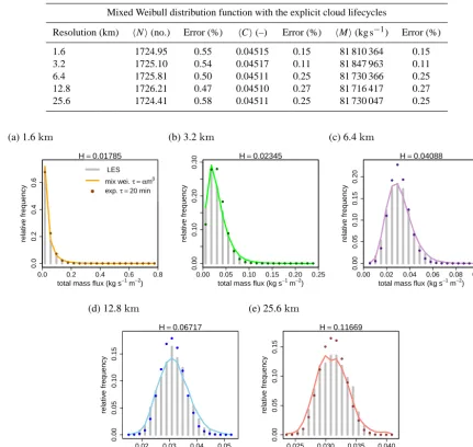
From the snapshots taken over six hours of simulation (6–12 h), the frequency distributions of the compound cloud mass flux at the 700 m height level are constructed for the different horizontal resolutions of the stochastic model and compared with the coarse-grained LES results (Fig. 9). It can be concluded, already by visual inspection, that the LES and the stochastic model frequency distributions are highly simi-lar. Limited sampling of the cloud ensemble produces a cor-rect frequency distribution of the subgrid convective states for the different choices of the model grid size. This signi-fies that the stochastic model is scale-adaptive and that the variability of small-scale convective states depends on the model grid resolution. There is a lack of variability when the cloud mass flux is sampled from an exponential func-tion with constant cloud lifetime (exp.τ =20 min, Fig. 9). This model set-up would correspond to the prescribed ex-ponential function for deep convection in PC-2008, with the constant cloud lifetimeτ=45 min. Thus, in a shallow con-vective case, a more complicated distribution function that encompasses the effect of cloud lifecycles should be used. This statement is supported by the improvement in perfor-mance of the stochastic model in the case of a mixed Weibull distribution including the explicit cloud lifecycles (mix wei.
τ=αmβ, Fig. 9). The reason for this improvement could be the generalisation of the cloud rate distribution, the introduc-tion of the second distribuintroduc-tion mode, the introducintroduc-tion of the cloud lifecycles, or a combination of all three. We examine all three reasons in the rest of the paper.
As a tool for quantitative comparison between the fre-quency distribution resulting from different runs of the stochastic model and the reference distribution obtained from the LES coarse graining, we use the Hellinger distance as a measure of distribution similarity. The Hellinger distance
H between the two discrete probability distributionsP and
Qis defined as
H (P , Q)=√1
2 v u u t
k
X
i=1
(√pi− √
qi)2, (33)
Table 4. Ensemble average cloud properties resulting from the stochastic model ensemble runs with the different horizontal resolutions.
Mixed Weibull distribution function with the explicit cloud lifecycles
Resolution (km) hNi(no.) Error (%) hCi(–) Error (%) hMi(kg s−1) Error (%)
1.6 1724.95 0.55 0.04515 0.15 81 810 364 0.15
3.2 1725.10 0.54 0.04517 0.11 81 847 963 0.11
6.4 1725.81 0.50 0.04511 0.25 81 730 366 0.25
12.8 1726.21 0.47 0.04510 0.27 81 716 417 0.27
25.6 1724.41 0.58 0.04511 0.25 81 730 047 0.25
(a) 1.6km
0.0 0.2 0.4 0.6 0.8
0.0
0.2
0.4
0.6
total mass flux (kgs−1m−2)
relativ
e frequency
H=0.01785
●
●
● ●
●●●●●●●●●●●●●●●● ●
LES
mix wei. τ = αmβ exp. τ =20 min
(b) 3.2km
0.000.00 0.05 0.10 0.15 0.20 0.25
0.10
0.20
0.30
total mass flux (kgs−1m−2)
relativ
e frequency
H=0.02345
● ●●
●
●
● ●
●●●●●●●●●●●●●
(c) 6.4km
0.000.00 0.02 0.04 0.06 0.08 0.10
0.05
0.10
0.15
0.20
total mass flux (kgs−1m−2)
relativ
e frequency
H=0.04088
●● ●
● ●
●
●
●
●
● ●
●●●●●●●●●
(d) 12.8km
0.02 0.03 0.04 0.05
0.00
0.05
0.10
0.15
total mass flux (kgs−1m−2)
relativ
e frequency
H=0.06717
●●● ●
● ●
● ●
●
●
●
●
●
● ●
●●●●●
(e) 25.6km
0.025 0.030 0.035 0.040
0.00
0.05
0.10
0.15
total mass flux (kgs−1m−2)
relativ
e frequency
H=0.11669
●●● ●
● ●
● ●
● ●
●
●
●
● ●
●●●●●
1
Figure 9. Histograms of the compound cloud mass flux at the 700 m height level normalised by the grid box area of the different horizontal resolution: coarse-grained LES tracking results vs. stochastic model results. Plots show the two stochastic model cases: a two-component
mixed Weibull case with explicit cloud lifecycles (k=0.7; coloured lines) and a single-mode exponential case without cloud lifecycles
(k=1; coloured dots). Colours also correspond to Fig. 5. Hellinger distanceHstands for the mixed Weibull case.
wherepi andqi are the corresponding probability measures.
A useful property of the Hellinger distance is its skew inde-pendence, which enables us to compare the scores between the distribution pairs of different skewness resulting from the different choice of horizontal grid resolution (Fig. 9).
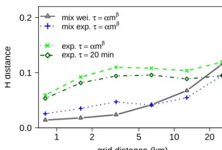
The Hellinger distance H confirms a high level of simi-larity between the distributions of different resolution pairs, with the H values in a very low range, from 0.018 to 0.12 (Fig. 9a–e). Comparison of the results from the stochastic model set-up using a single exponential function vs. a mixed exponential or a mixed Weibull function via Hellinger dis-tance shows the impordis-tance of modelling the two
distribu-tion modes for each cloud group separately (Fig. 10). For the distribution similarity, the introduction of the second mode in the cloud rate distribution (mix exp. vs. exp., Fig. 10) has a larger impact than the explicit modelling of the cloud lifecycles (exp.τ=αmβ vs. exp.τ =20 min, Fig. 10). The difference in performance of a mixed exponential case vs. a mixed Weibull case (i.e.k=1 vs.k=0.7) is not so evident from the point of view of frequency distribution match, but it becomes distinct for evaluation of the variability measure (see Sect. 4.2).