Estimation of Survival Function for Rayleigh Distribution by Ranking function:-

(1)

Baghdad Science Journal

Vol.16(3) Supplement 2019

775

DOI: http://dx.doi.org/10.21123/bsj.2019.16.3(Suppl.).0775

Estimation of Survival Function for Rayleigh Distribution by Ranking function:-

Iden H. Hussein

*

_{Hadeer A. KHammas}

Received 15/10/2018, Accepted 13/3/2019, Published 22/9/2019

This work is licensed under a Creative Commons Attribution 4.0 International License.

Abstract:

In this article, performing and deriving te probability density function for Rayleigh distribution is done by using ordinary least squares estimator method and Rank set estimator method. Then creating interval for scale parameter of Rayleigh distribution. Anew method using (𝑥̅ ±𝑠2) is used for fuzzy scale parameter. After that creating the survival and hazard functions for two ranking functions are conducted to show which one is beast.

Key words: Fuzzy number, Hazard function, Ordinary least squares estimator method, Rank set estimator method, Survival function.

Introduction:

One of the most popular functions in statistic is Rayleigh distribution which used in failure and survival times. Many authors tend to fuzzfiy data in studying some distribution as follows:-

In (2013) Pak and Saraj (1) studied two parameters of weibull distribution. In (2014) Pak and Saraj (2) studied the parameter of exponential distribution. In (2014) Shafiq and Viertl (3) used the maximum likelihood estimator for two parameters of weibull distribution. In (2016) Pak (4) studied inference for one parameter of lognormal distribution. In (2016) Jasim and Hussein (5) studied the two parameters of weibull distribution by using maximum likelihood method. In (2017) Shafiq (6) studied the two parameters of Pareto distribution. In (2017) Shafiq (7) studied statistical inference for the two parameters of Lindley distribution. The aim of this article is to estimate the parameter of Rayleigh distribution by using ordinary least squares method and rank set method then estimating the survival and hazard functions. After that, the researcher uses interval estimation to find the scale parameter of Rayleigh the distribution. The estimation is fuzzfied of scale parameter by using trapezoidal membership depending on ( 𝑥̅ +𝑠2) and ( 𝑥̅ −𝑠2) to fuzzify this parameter, then utilizing the ranking function procedure to transform the fuzzy parameter to crisp parameter.

Department of Applied Science, University of Technology, Baghdad, Iraq.

*_{Corresponding author: [email protected]}

Finally, the researcher estimates the fuzzy survival and hazard performance the compare between crisp and fuzzy survival functions by using mean square error to know which one is better.

Rayleigh Distribution:-

The Rayleigh distribution is widely used in Probability, Reliability, and Survival analysis. The Rayleigh distribution is as follows:-

𝑓(𝑡; 𝐵) = {𝐵𝑡 𝑒−

𝐵

2𝑡2 0 ≤ 𝑡 < ∞

0 𝑜. 𝑤 …. (1) Ω = {𝐵; 𝐵 > 0}, where 𝐵 is scale parameter. The cdf function of Rayleigh distribution is:- 𝐹(𝑡) = 1 − 𝑒−𝐵2𝑡2 _{…. (2)}

The survival function and hazard of Rayleigh distribution is:-

𝑆(𝑡) = 𝑒−𝐵2𝑡2 _{…. (3)}

ℎ(𝑡) = 𝐵𝑡 …. (4)

Ordinary Least Squares Method :-

The ordinary least squares method is one of the most popular procedures to estimate the

parameter 𝐵 in this distribution. The aim of the ordinary least square method is minimizing the sum squares of error.

In this method, the CDF of one-parameter Rayleigh distribution is used as follows:-

𝐹(𝑡𝑖) = 1 − 𝑒 − 𝐵 𝑡𝑖2

2 𝑡 ∈ [0, ∞)_{…. (5)}

(2)

ln[1 − 𝐹(𝑡_𝑖)] +𝐵𝑡𝑖2

2 = 0 …. (6)

𝑠(𝐵) = ∑ [ ln(1 − 𝐹(𝑡_𝑖)) +𝐵𝑡𝑖2 2 ]

2 𝑛

𝑖=1 …. (7)

Taking the partial derivatives for the above equation, then:-

𝜕𝑠(𝐵)

𝜕𝐵 = 2 ∑ [ 𝑛

𝑖=1 ln(1 − 𝐹(𝑡𝑖)) +𝐵𝑡𝑖 2

2 ] . 𝑡_𝑖2

2 …. (8) 𝜕𝑠(𝐵)

𝜕𝐵 = ∑ [𝑡𝑖 2 𝑛

𝑖=1 ln(1 − 𝐹(𝑡𝑖)) +𝐵𝑡𝑖 4

2 ] …. (9)

Equaling the partial derivative for log-likelihood with respect to zero, the equation is:- 𝜕𝑠(𝐵)

𝜕𝐵 =∑ [𝑡𝑖 2 𝑛

𝑖=1 ln(1 − 𝐹(𝑡𝑖)) +𝐵 ^_𝑡

𝑖 4

2 ] = 0 …. (10)

𝐵^₌−2 ∑𝑛𝑖=1ln(1−𝐹(𝑡𝑖))𝑡𝑖2

∑𝑛_𝑖=1𝑡_𝑖4 …. (11) Rank Set Method:-

Rank set sampling estimator method (RSS) was introduced by McIntyre for the first time in (1952) for estimating pasture yields.

The procurer to compute to estimator for Relight distribution is:-

𝑔(𝑦𝑖) =_{(𝑖−1)!(𝑛−𝑖)!}𝑛! [𝐹(𝑦𝑖)]𝑖−1[1 − 𝐹(𝑦𝑖)]𝑛−𝑖𝑓(𝑦𝑖 …. (12)

By using the p. d. f 0f one-parameter Rayleigh distribution is:-

𝑓(𝑡𝑖; 𝐵) = 𝐵𝑡𝑖𝑒− 𝐵𝑡𝑖2

2 …. (13)

Put 𝑓(𝑡𝑖; 𝐵) = 𝑓(𝑦𝑖; 𝐵)

where 𝑓(𝑦_𝑖; 𝐵) = 𝐵𝑦_𝑖𝑒− 𝐵𝑦𝑖

2

2 _{…. (14)}

The c .d .f of one –parameter Rayleigh distribution is:-

𝐹(𝑡_𝑖; 𝐵) = 1 − 𝑒− 𝐵𝑡𝑖

2

2 …. (15)

Therefore 𝐹(𝑡𝑖; 𝐵) = 𝐹(𝑦𝑖; 𝐵) …. (16)

𝐹(𝑦_𝑖; 𝐵) = 1 − 𝑒−𝐵𝑦𝑖

2

2 …. (17)

Let _{(𝑖−1)!(𝑛−𝑖)!}𝑛! = 𝑘 …. (18)

𝑔(𝑦_𝑖) = 𝑘 𝐵𝑦_𝑖[𝑒−𝐵𝑦𝑖

2

2 ]𝑛−𝑖+1 [1 − 𝑒−𝐵𝑦𝑖 2

2 ]𝑖−1 ….

(19)

The likelihood function of sample 𝑦1,𝑦2,𝑦3,,,,,,,,,,,𝑦𝑛 is: (20)

𝐿(𝐵; 𝑦_𝑖) =

𝑘𝑛_𝐵𝑛_∏ _𝑦 𝑖 𝑛

𝑖=1 𝑒− ∑ (𝑛−𝑖+1) 𝐵𝑦𝑖2

2 𝑛

𝑖=1 _{. ∏}𝑛 _{[1 −}

𝑖=1

𝑒− 𝐵𝑦𝑖

2

2 ]𝑖−1

Taking the loqarithm ofabove equation, getting : - (21)

𝑙𝑛 𝐿 = 𝑛 𝑙𝑛 𝑘 + 𝑛 𝑙𝑛 𝐵 + ∑ 𝑙𝑛 𝑦_𝑖

𝑛

𝑖=1

− ∑(𝑛 − 𝑖 + 1)𝐵𝑦𝑖

2

𝑛

𝑖=1

+ ∑(𝑖 − 1) 𝑙𝑛 [1 − 𝑒−𝐵𝑦𝑖

2 2 ] 𝑛

𝑖=1

Taking the partial derivatives for above equation, then: - (22)

𝜕 𝑙𝑛 𝐿 𝜕𝐵 =

𝑛

𝐵− ∑ (𝑛 − 𝑖 + 1) 𝑦_𝑖2

2 𝑛

𝑖=1 + ∑𝑛𝑖=1(𝑖 −

1)(−𝑒

−𝐵𝑦𝑖 2 2 −𝑦𝑖2

2 )

1−𝑒− 𝐵𝑦𝑖 2 2

equall above equation to zero as follows: −

𝜕 ln 𝐿 𝜕𝐵 =

𝑛

𝐵^− ∑ (𝑛 − 𝑖 + 1) 𝑦𝑖2

2 𝑛

𝑖=1 + ∑𝑛𝑖=1(𝑖 −

1) (𝑒−𝐵^𝑦𝑖 2 2 𝑦𝑖 2 2)

1−𝑒− 𝐵^𝑦𝑖 2 2

= 0 …. (23)

𝑔(𝑦𝑖 , 𝐵^) =_𝐵𝑛^− ∑ (𝑛 − 𝑖 + 1) 𝑦_𝑖2

2 𝑛

𝑖=1 +

∑ (𝑖 − 1)

(𝑒−𝐵^𝑦𝑖 2 2 𝑦𝑖

2

2)

1−𝑒− 𝐵^𝑦𝑖 2 2 𝑛

𝑖=1 …. (24)

This likelihood functions are difficult to be solved. It is impossible to find the estimate 𝐵. We use the numerical procedure to estimate 𝐵, that means using the following formula

𝐵̃_𝑘+1= 𝐵̃_𝑘− 𝑔(𝑦𝑖 , 𝐵)

𝑔′_(𝑦_𝑖_{, 𝐵)} …. (25)

𝑔′_(𝑦

𝑖 , 𝐵^) = −_𝐵𝑛^2+ ∑ (𝑖 − 1) −𝑦𝑖4 4 𝑒 −𝐵^𝑦𝑖 2 2 2

(1−𝑒−𝐵^𝑦𝑖 2 2 ₎ 2 𝑛 𝑖=1 …. (26)

- The interval estimation is as follows:-

[𝐵^− 𝑡√𝑣𝑎𝑟(𝐵^) , 𝐵^+ 𝑡√𝑣𝑎𝑟(𝐵^) ] …. (27)

Fuzzy Sets

(8):-Definition (1) (9): A crisp set is a special case of a fuzzy set, in which the membership function has only two values, 0 and 1.

Definition (2) (9): Let𝑥 be a nonempty set (universal set).A fuzzy set𝐴̃ in 𝑥 is characterized by its membership function 𝜇𝐴̃: 𝑥 → [0,1] 𝜇𝐴̃(𝑥) is the interpreted as a degree of membership of element 𝑥 in fuzzy set A for each 𝑥 ∈ 𝑋 and denoted for its set by 𝐴̃. 𝐴̃ = {(𝑥, 𝜇𝐴̃(𝑥): 𝑥 ∈ 𝑋}

(3)

Ranking Function (10):-

The method of ranking function was first introduced by Yager in (1981) proposed four indices that may be employed for the purpose of ordering fuzzy quantities in [0,1].

A ranking function is defined 𝑅: 𝐹(𝑅) → 𝑅, which maps each fuzzy number into the real line. Now, suppose that 𝑎 ̃and 𝑏̃ are two trapezoidal fuzzy numbers. Therefore, the orders on 𝐹(𝑅)are defined as following:-

(1) 𝑎 ̃ ≥𝑏̃ if and only if 𝑅(𝑎 ̃ ) ≥ 𝑅(𝑏̃) (2)𝑎 ̃ >𝑏̃ if and only 𝑅(𝑎 ̃ ) > 𝑅(𝑏̃)

(3)𝑎 ̃ =𝑏̃ If and only if 𝑅(𝑎 ̃ ) = 𝑅(𝑏̃) where 𝑎 ̃and 𝑏̃ are in 𝐹(𝑅). Also

𝑎 ̃ ≤𝑏 ̃If and only if 𝑎 ̃ ≥𝑏̃

Lemma:-(10) let R be any linear ranking function then:-

i- 𝑎 ̃ ≥𝑏̃ iff −𝑏̃ ≥ 0 iff −𝑏̃ ≥ 𝑎 ̃ ii- if 𝑎 ̃ ≥𝑏̃ and 𝑐 ̃ ≥𝑑,̃ then 𝑎 ̃ +𝑐̃≥𝑑̃

+𝑏̃

Algorithms of the Ranking Function:- The First Algorithm:-

Yager (1981) (11) studied the ranking function, 𝑅: 𝐹(𝑅) → 𝑅

Let 𝐴̃ = (𝑎, 𝑏, 𝑐, 𝑑) be trapezoidal fuzzy number, and then the following formula is applied to find the ranking function of 𝐴̃

𝑅(𝐴̃) =1₂ ∫ (𝑖𝑛𝑓𝐴̃₀1 𝜇+ 𝑠𝑢𝑝𝐴̃𝜇) 𝑑𝜇

Let 𝜇4 =(𝑥−𝑎)

𝑏−𝑎 by using inverse transformation:-

𝜇4_{(𝑏 − 𝑎)}₌_{(𝑥 − 𝑎)}

𝑥 = 𝜇4_{(𝑏 − 𝑎) + 𝑎 = 𝑖𝑛𝑓𝐴̃} 𝜇

𝜇2 ₌(𝑑−𝑥)

(𝑑−𝑐) by using inverse transformation

𝜇2_{(𝑐 − 𝑑)}₌_{(𝑥 − 𝑑)}

𝑥 = 𝜇2_{(𝑐 − 𝑑) + 𝑑 = 𝑠𝑢𝑝𝐴̃} 𝜇

𝑅(𝐴̃) =1₂ ∫ (₀1 𝜇4_{𝑏 − 𝜇}4_{𝑎 + 𝑎 ) 𝑑𝜇 + ∫ (}1 0 𝜇2𝑐 −

𝜇2_{𝑑 + 𝑑 ) 𝑑𝜇}

𝑅(𝐴̃) =₃₀1 [3𝑏 + 12𝑎 + 5𝑐 + 10𝑑] …. (28)

The Second Algorithm:-

Maleki (2002) studied the ranking function, 𝑅: 𝐹(𝑅) → 𝑅

Let 𝐴̃ = (𝑎, 𝑏, 𝑐, 𝑑) be trapezoidal fuzzy number, and then the following formula is applied to find the ranking function of 𝐴̃

𝑅(𝐴̃) =1₂ ∫ (𝑖𝑛𝑓𝐴̃₀1 𝜇+ 𝑠𝑢𝑝𝐴̃𝜇) 𝑑𝜇

𝜇 =(𝑥−𝑎)_𝑏−𝑎 by using inverse transformation:- 𝜇 (𝑏 − 𝑎)= (𝑥 − 𝑎)

𝑥 = 𝜇 (𝑏 − 𝑎) + 𝑎 = 𝑖𝑛𝑓𝐴̃_𝜇

𝜇 =(𝑑−𝑥)_{(𝑑−𝑐)} by using inverse transformation 𝜇 (𝑐 − 𝑑)= (𝑥 − 𝑑)

𝑥 = 𝜇 (𝑐 − 𝑑) + 𝑑 = 𝑠𝑢𝑝𝐴̃𝜇

𝑅(𝐴̃) =1₂ ∫ ( 𝜇 (𝑏 − 𝑎) + 𝑎 +₀1 𝜇 (𝑐 − 𝑑) + 𝑑) 𝑑𝜇 𝑅(𝐴̃) =1₄[ 𝑏 + 𝑎 + 𝑐 + 𝑑] …. (29) Definition (4) (11): The support of a fuzzy set 𝐴̃, 𝑆(𝐴̃) is the crisp set of all 𝑥 ∈ 𝑋 such that 𝜇_𝐴̃ > 0 i.e. supp(𝐴̃) = {𝑥 ∈ 𝑋: 𝜇𝐴̃(𝑥) > 0}

Definition (5) (11):-The height h (A) of a fuzzy set 𝐴 is the largest membership grade obtained by any element in that set, formally, ℎ(𝐴) = 𝑠𝑢𝑝𝑥∈𝑋 𝐴(𝑥) Definition (6) (11): The elements of 𝑥, such that 𝜇_𝐴̃(𝑥) =1₂ are called crossover points of 𝐴̃.

Definition (7) (11): The crisp set of element that belongs to the fuzzy set 𝐴̃ at least to the degree ∝ is called the ∝ -level set that is:- 𝐴∝ =

{𝑥 ∈ 𝑋: 𝜇_𝐴̃≥∝}

𝐴∝′ = {𝑥 ∈ 𝑋: 𝜇𝐴̃>∝} Is called strong ∝ - level set or strong ∝-cut.

Trapezoidal Function:-(11)

A fuzzy number 𝐴̃(𝑎, 𝑏, 𝑐, 𝑑; 1) is said to be a trapezoidal fuzzy number if its membership function is given by:-

𝜇_𝐴̃(𝑥)

=

{

(𝑥 − 𝑎)

𝑏 − 𝑎 , 𝑎 ≤ 𝑥 < 𝑏 1 , 𝑏 < 𝑥 ≤ 𝑐 (𝑑 − 𝑥)

(𝑑 − 𝑐) , 𝑐 < 𝑥 ≤ 𝑑 0 𝑜𝑡ℎ𝑒𝑟𝑤𝑖𝑠𝑒

Mean Time To failure:-

MTTF=∫ 𝑠(𝑡) 𝑑𝑡₀∞ , MTTF=∫ 𝑒−

𝐵 2𝑡2 𝑑𝑡 ∞

0 Let u=𝐵₂𝑡2, 𝑑𝑢 =_{√𝐵√2𝑢}1

MTTF=∫ 𝑒−𝑢_√𝐵√21 𝑢−

1 2𝑑𝑢 ∞

0

MTTF=_√𝐵√2√𝜋 …. (30) - The mean squared error by following equation is:-

MSE [𝑆^(𝑡𝑖)] = ∑ [𝑆 ^_(𝑡

𝑖)−𝑆(𝑡𝑖)]2 𝑛 𝑛

𝑖=1 …. (31) Where: - 𝑆^_(𝑡

𝑖) Is estimated survival function, 𝑆(𝑡𝑖) is empirical survival which:-

𝑆(𝑡_𝑖) =𝑖−0.5

𝑛

Application:-

(4)

and forty eight patients remained alive, this means the data became complete data are (20) patients

where:-T=[15,22,26,30,35,42,44,58,60,65,66,71,73,75,80,8 6,91,104,121,190]

(a) – Ordinary Least Squares Method:- * The value of𝐵^ from equation (11) is:- 𝐵^= 0.00026

* f(t), s(t), h(t) from equations (1), (3), (4) then tabulating in following table:-

Table 1. Estimate value for functions

𝒇(𝒕), 𝑺(𝒕), 𝒉(𝒕) functions

T f(t) S(t) h(t)

15 0.0038 0.9711 0.0039

22 0.0054 0.9389 0.0057

26 0.0062 0.9157 0.0068

30 0.0070 0.8894 0.0078

35 0.0078 0.8525 0.0091

42 0.0087 0.7947 0.0109

44 0.0089 0.7771 0.0115

58 0.0097 0.6452 0.0151

60 0.0098 0.6257 0.0156

65 0.0098 0.5768 0.0169

66 0.0097 0.5670 0.0172

71 0.0096 0.5186 0.0185

73 0.0095 0.4995 0.0190

75 0.0094 0.4806 0.0195

80 0.0091 0.4345 0.0208

86 0.0085 0.3816 0.0224

91 0.0081 0.3401 0.0237

104 0.0066 0.2445 0.0271

121 0.0047 0.1485 0.0315

190 0.0004 0.0091 0.0495

-By applying the equation (30) is: - MTTF=77.7075 - By applying the equation (31) is: - MSE

[𝑆^(𝑡𝑖)] =0.3117

* To find the interval estimation applying the equation (27) as follows:-

𝐵^_{= [0.00013,0.00038]}_{= [a, d]} * Then applying ( 𝑥̅ −𝑠2) = 𝑏 and ( 𝑥̅ +𝑠2) = 𝑐, therefore the trapezoidal becomes as 𝐵^_{= [0.00013,0.00024,0.00025,0.00038]} (1)- applying the first ranking function by using equation (28) as follow:-

𝐵^_{= 0.00024}

Finding the f(t), s(t), h(t) and tabulating in following table:-

T f(t) S(t) h(t)

15 0.0035 0.9734 0.0036

22 0.0050 0.9436 0.0053

26 0.0058 0.9221 0.0062

30 0.0065 0.8976 0.0072

35 0.0073 0.8633 0.0084

42 0.0082 0.8092 0.0101

44 0.0084 0.7927 0.0106

58 0.0093 0.6679 0.0139

60 0.0093 0.6492 0.0144

65 0.0094 0.6023 0.0156

66 0.0094 0.5929 0.0158

71 0.0093 0.5461 0.0170

73 0.0092 0.5276 0.0175

75 0.0092 0.5092 0.0180

80 0.0089 0.4639 0.0192

86 0.0085 0.4117 0.0206

91 0.0081 0.3702 0.0218

104 0.0068 0.2731 0.0250

121 0.0050 0.1726 0.0290

190 0.0006 0.0131 0.0456

- By applying the equation (30) is: - MTTF=80.8806

- By applying the equation (31) is: - MSE [𝑆^(𝑡𝑖)] =0.3089

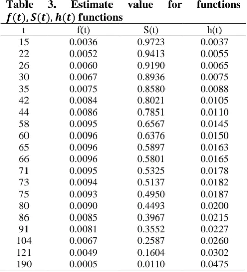
* (2) applying the second ranking function method by using equation (29) as follow:- 𝐵^= 0.00025 Finding the f (t), s (t), h (t) and tabulating in following table:-

t f(t) S(t) h(t)

15 0.0036 0.9723 0.0037

22 0.0052 0.9413 0.0055

26 0.0060 0.9190 0.0065

30 0.0067 0.8936 0.0075

35 0.0075 0.8580 0.0088

42 0.0084 0.8021 0.0105

44 0.0086 0.7851 0.0110

58 0.0095 0.6567 0.0145

60 0.0096 0.6376 0.0150

65 0.0096 0.5897 0.0163

66 0.0096 0.5801 0.0165

71 0.0095 0.5325 0.0178

73 0.0094 0.5137 0.0182

75 0.0093 0.4950 0.0187

80 0.0090 0.4493 0.0200

86 0.0085 0.3967 0.0215

91 0.0081 0.3552 0.0227

104 0.0067 0.2587 0.0260

121 0.0049 0.1604 0.0302

190 0.0005 0.0110 0.0475

-By applying the equation (30) is: - MTTF=79.2465 - By applying the equation (31) is: - MSE

(5)

(b)-Rank Set Method:-

* The value of𝐵^ from equation (25) 𝐵^_{= 0.00036}

* f(t), s(t), h(t) from equations (1), (3), (4) then tabulating in following table:-

T f(t) S(t) h(t)

15 0.0052 0.9599 0.0055

22 0.0073 0.9158 0.0080

26 0.0084 0.8844 0.0095

30 0.0093 0.8491 0.0109

35 0.0102 0.8004 0.0127

42 0.0111 0.7257 0.0153

44 0.0113 0.7034 0.0160

58 0.0114 0.5426 0.0211

60 0.0113 0.5198 0.0218

65 0.0110 0.4640 0.0236

66 0.0109 0.4531 0.0240

71 0.0103 0.4000 0.0258

73 0.0101 0.3796 0.0265

75 0.0098 0.3597 0.0273

80 0.0091 0.3125 0.0291

86 0.0082 0.2607 0.0313

91 0.0073 0.2220 0.0331

104 0.0053 0.1400 0.0378

121 0.0031 0.0699 0.0440

190 0.0001 0.0014 0.0691

* To find the interval estimation applying the equation (27) as follows:-

𝐵^_{= [0.00019,0.00052] = [𝑎, 𝑑 ]} * Then applying ( 𝑥̅ −𝑠2) = 𝑏 and (𝑥̅ +𝑠2) = 𝑐, therefore the trapezoidal becomes as follow:- 𝐵^_{= [0.00019,0.00034,0.00035,0.00052]} (1)- applying the first ranking function by using equation (28) as follow:-

𝐵^_{= 0.00034}

Finding the f(t), s(t), h(t) and tabulating in following table:-

T f(t) S(t) h(t)

15 0.0049 0.9625 0.0051

22 0.0069 0.9210 0.0075

26 0.0079 0.8914 0.0088

30 0.0088 0.8581 0.0102

35 0.0097 0.8120 0.0119

42 0.0106 0.7409 0.0143

44 0.0108 0.7196 0.0150

58 0.0111 0.5645 0.0197

60 0.0111 0.5423 0.0204

65 0.0108 0.4876 0.0221

66 0.0107 0.4769 0.0224

71 0.0102 0.4244 0.0241

73 0.0100 0.4042 0.0248

75 0.0098 0.3843 0.0255

80 0.0092 0.3369 0.0272

86 0.0083 0.2844 0.0292

91 0.0076 0.2447 0.0309

104 0.0056 0.1590 0.0354

121 0.0034 0.0830 0.0411

190 0.0001 0.0022 0.0646

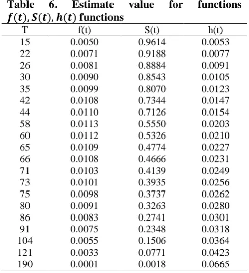
* (2) applying the second ranking function method by using equation (29) as follow:- 𝐵^= 0.00035 Finding the f(t), s(t), h(t) and tabulating in following table:-

T f(t) S(t) h(t)

15 0.0050 0.9614 0.0053

22 0.0071 0.9188 0.0077

26 0.0081 0.8884 0.0091

30 0.0090 0.8543 0.0105

35 0.0099 0.8070 0.0123

42 0.0108 0.7344 0.0147

44 0.0110 0.7126 0.0154

58 0.0113 0.5550 0.0203

60 0.0112 0.5326 0.0210

65 0.0109 0.4774 0.0227

66 0.0108 0.4666 0.0231

71 0.0103 0.4139 0.0249

73 0.0101 0.3935 0.0256

75 0.0098 0.3737 0.0262

80 0.0091 0.3263 0.0280

86 0.0083 0.2741 0.0301

91 0.0075 0.2348 0.0318

104 0.0055 0.1506 0.0364

121 0.0033 0.0771 0.0423

190 0.0001 0.0018 0.0665

(6)

-By applying the equation (31) is: - MSE [𝑆^(𝑡𝑖)] =0.3250

- Algorithms Comparison:-

Algorithm MTTF MSE

Crisp{𝑂𝐿𝑆

𝑅. 𝑆 {77.707566.0387 {0.31170.3265 First Algorithm

{𝑂𝐿𝑆_{𝑅. 𝑆} {80.880667.9533 {0.30890.3235 second Algorithm

{𝑂𝐿𝑆_{𝑅. 𝑆} {79.246566.9755 {0.31030.3250

-Noting that from above table, that minimum mean squares error is of first algorithm of ordinary least squares method but the high mean squares error is crisp of rank set method. Therefor the mean time of failure the first algorithm of ordinary least squares method, but the minimum mean time to failure is crisp of rank set method.

Conflicts of Interest: None.

References:

-

1. Pak A, Parham GA, Saraj M. Inference for the weibull distribution bases on fuzzy data evista Columbiana de Estadistica. 2013;2 (36) : 339-358

2. Pak A, Parham GA, Saraj M. Inference on the competing Risk Reliability problem for exponential distribution based on fuzzy data .IEEE Transactions on Reliability. 2014.; 6 (3) :2-12

3. Shafiq M, Viertl R. Maximum likelihood Estimation for weibull distribution in case of censored Fuzzy lifetime data. Vienna university of Technology. 2014.:1-17

4. Pak A .Inference for the shape parameter of lognormal distribution in presence of fuzzy data. Pakistan Journal of statistics and operation Research . 2016.;12( 1) :89 -99

5. Jasim ZF, Hussein IH. fuzzy Reliability function estimation for weibull distribution. 2016.;7: 355-366. 6. Shafiq M. Classical and Bayesian inference of pareto

distribution and fuzzy lifetime. Pak. J. statist. 2017.; 33:15-25

7. Shafiq M. statistical inference for the parameter of Lindley distribution based on fuzzy data. Braz. J. probab. stat. 2017.;31(3): 502-515

8. Selvakumari K, Lavanya S. An Approach for Solving Fuzzy Game problem. Indian Journal of Science and Technology. 2015.;8(15):2-6

9. Zimmermann H J. Fuzzy Set Theory. Journal of Advanced Review. 2010.; 2: 317-332

10.Maleki HR. Ranking function and their Application to Fuzzy linear programming. far eastJ. Math. Sci. 2002.; 4:283-301.

11.Yager RR. A Procedure for Ordering Fuzzy Subsets of the unit Interval. Information Sciences. 1981; 24:227-242.

ةيبترلا ةلادلا مادختساب يلار عيزوتل ءاقبلا ةلاد ريدقت

سامخ دمحأ ريده نيسح نسح نديا

.قارعلا ،دادغب ،دادغب ةعماج ،تانبلل مولعلا ةيلك ،تايضايرلا مسق

:ةصلاخلا

اذه يف ، ىرغصلا تاعبرملا طسوتم ةقيرط( مادختساب عيزوتلا اذه ةملعم ريدقت للاخ نم يلار عيزوتل ءاقبلا ةلاد ريدقت مت ثحبلا

ضعب مادختساب ءاقبلا ةلاد ريدقت متو ببضملا عيزوتلا ىلا عيزوتلا اذه ليوحتل فرحنملا هبش ةيوضعلا ةلاد مادختسا متو ) ةيبترلا ةقيرط لاودلا

متو ةيبترلا .ةيقبلا نم لضفلاا نم ةفرعمل ءاقبلا لاودل أطخلا تاعبرم طسوتم مادختسا

:ةيحاتفملا تاملكلا ةيبابضلا دادعلاا