www.earth-syst-dynam.net/6/731/2015/ doi:10.5194/esd-6-731-2015
© Author(s) 2015. CC Attribution 3.0 License.
Quantifying differences in land use emission estimates
implied by definition discrepancies
B. D. Stocker1and F. Joos2,3
1Department of Life Sciences, Imperial College London, Silwood Park, Ascot, SL5 7PY, UK 2Climate and Environmental Physics , Physics Institute, University of Bern, Bern, Switzerland
3Oeschger Centre for Climate Change Research , University of Bern, Bern, Switzerland
Correspondence to: B. D. Stocker ([email protected])
Received: 5 March 2015 – Published in Earth Syst. Dynam. Discuss.: 19 March 2015 Revised: 4 November 2015 – Accepted: 10 November 2015 – Published: 27 November 2015
Abstract. The quantification of CO2 emissions from anthropogenic land use and land use change (eLUC) is
essential to understand the drivers of the atmospheric CO2increase and to inform climate change mitigation
pol-icy. Reported values in synthesis reports are commonly derived from different approaches (observation-driven bookkeeping and process-modelling) but recent work has emphasized that inconsistencies between methods may imply substantial differences ineLUC estimates. However, a consistent quantification is lacking and no concise modelling protocol for the separation of primary and secondary components ofeLUC has been established. Here, we review differences ofeLUC quantification methods and apply an Earth System Model (ESM) of Intermediate Complexity to quantify them. We find that the magnitude of effects due to merely conceptual differences between ESM and offline vegetation model-based quantifications is∼20 % for today. Under a future business-as-usual scenario, differences tend to increase further due to slowing land conversion rates and an increasing impact of altered environmental conditions on land-atmosphere fluxes. We establish how coupled Earth System Models may be applied to separate secondary component fluxes ofeLUC arising from the replacement of potential C sinks/sources and the land use feedback and show that secondary fluxes derived from offline vegetation models are conceptually and quantitatively not identical to either, nor their sum. Therefore, we argue that synthesis stud-ies should resort to the “least common denominator” of different methods, following the bookkeeping approach where only primary land use emissions are quantified under the assumption of constant environmental boundary conditions.
1 Introduction
Anthropogenic emissions of CO2are the main driver for
ob-served climate change (Stocker et al., 2013b) and primar-ily result from the combustion of fossil fuels and anthro-pogenic land use and land use change (LUC) (Le Quéré et al., 2015). Conceptually, fossil fuel emissions can be regarded as an external forcing acting upon the C cycle-climate sys-tem. In contrast, LUC additionally modifies the response of terrestrial ecosystems to elevated CO2 and changes in
cli-mate (Gitz and Ciais, 2003; Strassmann et al., 2008) and thereby affects the C cycle-climate feedback (Joos et al., 2001; Friedlingstein et al., 2006; Stocker et al., 2013a). This leaves room for interpretations as to how exactly land use
change emissions (eLUC) are to be defined and where the system boundaries are to be drawn.
The definition ofeLUC is relevant for the accounting of the global C budget (Ciais et al., 2013). Top-down derived land-atmosphere C fluxes that are not explained by bottom-up estimates ofeLUC are commonly ascribed to the residual
terrestrial C sink. Differences in the definition ofeLUC thus
directly translate into differences in estimates for the resid-ual terrestrial C sink. This budget term is a major source of uncertainty in climate projections (Jones et al., 2013) and its quantitative understanding motivates a large part of current research in biogeochemistry and terrestrial ecology.
Common to almost all approaches to quantify “CO2
models, is that eLUC is calculated as the difference in the global total land-to-atmosphere flux (F) between a realistic world where land vegetation cover and C pools are affected by prescribed, time-varying LUC maps (subscript LUC) and a hypothetical world, where no LUC is occurring (sub-script 0):
eLUC=FLUC−F0. (1)
However, the definition or model setup, under which FLUC
andF0are calculated, is relevant as it implies the inclusion
of secondary fluxes. Strassmann et al. (2008) (henceforth termed SM08) laid out a framework to distinguish between different component fluxes arising from land use, including primary emissions from converted land, and secondary emis-sions arising from the interactions between climate, CO2and
LUC. Pongratz et al. (2014) (henceforth termed PG14) show that numerous different definitions ofeLUC have been used in the published literature, implying a bewildering array of different combinations of component fluxes that are counted towards eLUC in the different studies. SM08 and PG14 demonstrate conceptually that due to this, typicaleLUC es-timates derived from observation-driven bookkeeping mod-els, offline Dynamic Global Vegetation Modmod-els, and coupled Earth System Models give systematically different results.
Substantial, setup-related differences in eLUC estimates have been found in earlier studies (Strassmann et al., 2008; Arora and Boer, 2010; Gasser and Ciais, 2013), and dif-ferent component fluxes have been identified and quantita-tively separated within their respective modelling framework (Gitz and Ciais, 2003; Strassmann et al., 2008). SM08 dis-tinguished between primary emissions that capture the di-rect effects of land conversion, and secondary effects aris-ing from the interaction of land conversion and environmen-tal change (CO2 and climate). SM08 further separated the
secondary fluxes into the land use feedback flux and the
re-placed sinks/sources flux. We term these eLFB and eRSS,
respectively, and provide definitions in Sect. 3 and quantifi-cations in Sect. 5. Recently, Gasser and Ciais (2013) (GC13) provided quantitative estimates of historical eLUC follow-ing different definitions. However, their analysis is limited to offline vegetation model quantifications and thus cannot ad-dress the aforementioned discrepancies between offline and ESM methods.
Here, we apply a single model, use a simple formalis-tic description ofeLUC flux components inspired by GC13 and SM08, and follow the classification of PG14 to distin-guish different methods of eLUC quantification. We quan-tify these differences for the historical period and a future business-as-usual scenario (RCP8.5). In contrast to earlier studies (Strassmann et al., 2008; Arora and Boer, 2010), we designed model setups to limit differences ineLUC to merely conceptual ones by using climate and CO2outputs from the
coupled simulations to drive offline simulations, instead of using observational data for the latter. We will demonstrate
that such definition differences imply inconsistencies of esti-mated land use emissions on the order of 20 % on the global scale and may increase to 30 % under a future business-as-usual scenario. This is directly relevant for territorial C bal-ance accounting and national greenhouse gas balbal-ances under the Kyoto Protocol and thus inherently carries a political rel-evance.
We elucidate the implications of the choice of defini-tion for the residual terrestrial C sink and global C bud-get accounting and discuss howeLUC quantifications may most appropriately be defined in studies that rely on mul-tiple methodological approaches. In such cases, we pro-pose, following Houghton (2013), to resort to the “least common denominator”, following the bookkeeping approach (method D1 in PG14), where LUC emissions are defined without accounting for any indirect effects on terrestrial C storage caused by transient changes in CO2or climate.
2 Brief overview of methods D1, D3, and E2
We start by revisiting the classification of PG14 for a subset ofeLUC quantification methods identified in their study. We focus our analysis on the discrepancy betweeneLUC derived from bookkeeping and offline vegetation models (D1 and D3 methods) and coupled ESMs (E2 method). Results of the D3 method feature prominently in model intercompar-ison studies (McGuire et al., 2001; Sitch et al., 2008), the Global Carbon Project (Le Quéré et al., 2015) and the IPCC (Ciais et al., 2013), and are often presented along with and compared against D1-type estimates. Yet, a consistent sepa-ration of commonly identified component fluxes can only be achieved by ESMs (see below).
2.1 Bookkeeping method (D1)
The first global quantifications of CO2emissions from LUC
were based on bookkeeping models that track the fate of C af-ter conversion from natural to cropland or pasture vegetation or vice versa (Houghton et al., 1983). Updated bookkeep-ing estimates ofeLUC (Houghton, 1999; Houghton et al., 2012) still represent the benchmark against which process-based models with prognostic vegetation C density are often compared (Le Quéré et al., 2015). Bookkeeping models use observational information of C density in natural and agri-cultural vegetation and in different biomes to calculateeLUC (Houghton et al., 1983). Environmental boundary conditions thus implicitly represent fixed conditions under which the ob-servations are taken, i.e. climate, CO2, and N-deposition
land-to-atmosphere carbon flux (F) between a simulation with and one without LUC (method D1; see Eq. 2). Here, these con-ceptually comparable methods are both referred to as book-keeping method. For method D1 it holds
eLUCD1=FLUC0 −F00. (2)
In general,Frefers to a global annual flux, but equations pro-vided here are valid also for cumulative fluxes and smaller spatial domains. Constant environmental boundary condi-tions (CO2, climate, nitrogen deposition etc.) in both
sim-ulations are reflected by superscript “0”. F00 is the land-atmosphere flux in the reference state, which may either be forced with the land use distribution at the beginning of the transient simulation (year 1700 here, see Sect. 4) or zero an-thropogenic land use. This choice affects secondary fluxes. Models are commonly spun up to equilibrate C pools and henceF00is zero except for net land-atmosphere CO2fluxes
occurring due to unforced climate variability.
Internal, unforced climate variability may affect the quan-tification of eLUC as climate variability affects the land-atmosphere carbon flux F. Ideally, the model setup should be such that internal, unforced variability evolves identically in both simulations. Then the land-atmosphere fluxes from land not affected by LUC and caused by internal variability would cancel when evaluating Eq. (2). In practice, this may be difficult to achieve for some state-of-the-art Earth System Models as LUC affects heat and water fluxes and thus cli-mate. A potential solution is to run the land module offline in both simulations or to force the land module in the simu-lation with LUC by using climate output from the reference simulation without LUC.
eLUCdI is equivalent to primary emissions (see Sect. 3) and captures instantaneous CO2emissions occurring during
deforestation and C uptake during regrowth, as well as de-layed (legacy) emissions from wood product decay and the gradual re-adjustment of soil and litter C stocks to altered input levels and turnover times. Depending on the model, eLUCdI may also include effects of shifting cultivation (cy-cle of cutting forest for agriculture, then abandoning) and wood harvest.eLUCdI is determined by the spatio-temporal information of land use change, C inventories in natural and agricultural land and the response timescales of C pools after conversion.
2.2 Climate and CO2-driven offline models (D3 method) Prognostically simulating vegetation C density instead of prescribing it has the advantage that secondary effects under environmental change can be simulated. The first such study using a set of process-based vegetation models with pre-scribed, transiently varying climate and CO2from observed
historical data was presented by McGuire et al. (2001). This method is termed D3 following the classification of PG14 and is also referred to as an “offline” setup, commonly
applied to stand-alone Dynamic Global Vegetation Mod-els (DGVM) or Terrestrial Ecosystem ModMod-els (TEM).
eLUCD3=FLUCFF+LUC−F0FF+LUC (3)
Here, the superscripts indicate that actually observed, time-varying environmental conditions (climate, CO2,
N-deposition, etc.) are the result of fossil fuel emissions and other non-LUC related forcings (FF), and land use change (LUC), and are prescribed in the LUC and in the non-LUC simulation. This also corresponds to the setup used in GC13 for quantifying “emissions from land use change”. Their “CCN” perturbation is analogous to what the super-script “FF+LUC” represents.
2.3 Emission-driven coupled Earth System Models (E2) For a consistent separation of total CO2emissions related to
LUC, emission-driven, coupled Earth System Models (ESM) may be applied. In such a setup, climate and atmospheric CO2 interactively evolve in response to anthropogenic land
use change, fossil fuel emissions, and other forcings. This method is termed E2 following the classification of PG14 and is typically computed with ESM or simpler atmosphere– ocean–land climate-carbon models:
eLUCE2=FLUCFF+LUC−F0FF. (4)
Here, the superscript “FF” corresponds to the environmen-tal conditions simulated with prescribed fossil emissions and other non-LUC related anthropogenic or natural forc-ing, whereas superscript “FF+LUC” refers to a simulation where environmental conditions evolve interactively in re-sponse to LUC-related emissions, as well as the “FF” forc-ing. As noted also in earlier publications (Strassmann et al., 2008; Arora and Boer, 2010; Pongratz et al., 2014), here, in contrast to the D3 method, environmental conditions in the LUC and non-LUC simulation differ. In the non-LUC case, climate and CO2are consistent with absent LUC, and
hence CO2is lower in the non-LUC simulation. This implies
a systematic difference in flux quantifications following the D3 and E2 methods. This difference may be expressed as flux components that are either ascribed to total eLUC or not. Below, we will identify a set of commonly defined flux components and investigate the discrepancies between meth-ods D1, D3, and E2 conceptually (Sect. 3) and quantitatively (Sect. 5).
averaging over a large spatial domain and temporal smooth-ing tends to moderate the influence of unforced variability on eLUCeII.
3 Defining flux components
SM08, PG14, and GC13 establish a formalism to de-scribe and discuss the different definitions of total eLUC and its component fluxes. Here, we synthesize these previous frameworks to a minimal description that al-lows us to identify the different flux components con-tained in eLUC provided by the offline DGVM setups (D3 method), coupled ESM model setups (E2 method), and the bookkeeping approach (D1 method). We then show that eLUCE2=eLUC0+eRSS+eLFB plus synergy terms. We
propose a definition for the delineation between component fluxes that follows a separation along underlying drivers of environmental changes, and that allows a consistent identi-fication of component fluxes in coupled model setups with and without the FF forcing. The formalism presented below sets the basis for the analysis and discussion in subsequent sections.
A reference time (or period) t0is selected. Att0all land
with total areaA0is “undisturbed” with respect to land use
changes that take place aftert0. The reference areaA0may
include agricultural land that was converted before t0. Net
atmosphere-land carbon fluxes att0 and thereafter may not
vanish as the land system may not be in equilibrium with the atmosphere. Under commonly used model setups, the extent of agricultural land in the reference state is small in com-parison to the area under natural vegetation. Similarly, mod-els are typically spun-up towards equilibrium and remaining trends in atmosphere-land fluxes are small. For simplicity, we neglect these disequilibrium fluxes below.
Additional fluxes arise due to forcings that occur after the reference time. We separate forcings into a land use change (LUC) and a non-land use change component (FF) such as fossil fuel emissions, nitrogen deposition, ozone changes etc. In a simulation without LUC, these addi-tional fluxes occur on undisturbed land (subscript “und”) and are caused by FF (use of superscript analogous as in Eqs. 3 and 4) and we write F0FF(t)=A01fundFF(t). 1
de-notes a change in a variable relative to the reference time t0(e.g.1f(t)=f(t)−f(t0)). Note thatfFF(t0) is zero by
definition. Below, we drop the specification of t. In a sim-ulation with LUC, we can write fluxes occurring over land that has not been converted since the reference timet0
(sub-script “und”) and land that has been converted aftert0
(sub-script “dis”) as
FLUCFF+LUC=(A0−1A)1fundFF+LUC
| {z }
undisturbed land
+1Af0+1fdisFF+LUC
| {z }
disturbed land
. (5)
1Ais the total area that has been converted, e.g. from natural to cropland or vice versa, since the reference time and up to
the point in time of interest. Note that disturbed and undis-turbed land both “see” the environmental forcing caused by FF and LUC. GC13 treat fluxes on disturbed land as a vec-tor representing land area cohorts that have transitioned from natural to agricultural land at a given time. Here, we drop the vector notation for individual age cohorts after conver-sion and lump these into a scalar representing non-natural (agricultural) land of varying age (1A(f0+1fdisFF+LUC)). f0 are direct emissions in response to land conversion un-der constant environmental conditions and comprise instan-taneous and legacy fluxes due to LUC aftert0as identified by IuandLuin PG14;1fdisFF+LUCis its modification due to
en-vironmental change (δI andδLin PG14). Note that on long timescales, the cumulative flux of (1fdisFF+LUC) is indepen-dent of the magnitude off0.
Using Eq. (4) and1fFF+LUC=1fFF+1fLUC+δ al-lows us to expand and re-arrange terms in Eq. (5) and to write the total C flux induced by LUC aftert0as a sum of
commonly separated component flux components, primary emissions (eLUCo), replaced sinks/sources (eRSS), and the land use feedback flux (eLFB) plus synergy terms:
eLUCE2=FLUCFF+LUC−F0FF (6)
=1A 1fdisFF−1fundFF (eRSS) (7)
+(A0−1A)1fundLUC+1A1f LUC
dis (eLFB) (8)
+1Af0 (eLUC0) (9)
+(A0−1A)δund+1Aδdis (synergy). (10)
We emphasize that eLUC includes only those fluxes due to land conversion after the reference time. Any legacy fluxes from land conversion before t0 are not included.
Atmosphere-land fluxes arising from a disequilibrium att0
affectFLUCFF+LUCandF0FFand thus cancel, apart from synergy terms.A01fundFF is the land-atmosphere flux in a simulation
forced only by FF and can be interpreted as the potential land C sink (ePS) under environmental change caused by FF.
ePS=A01fundFF. (11)
The above definition (Eqs. 6–10) of the total C flux induced by LUC corresponds to the E2 method, eLUCE2 (Eq. 4). eLUC0 are primary emissions and equivalent to eLUCD1,
as quantified using a bookkeeping approach. Analogously, component fluxes of the land-atmosphere CO2exchange in
the different model setupsFikcan now be identified (see Ta-ble 2).
In spite of the variety of terminologies presented in the published literature, studies generally agree that total C fluxes induced by LUC can be split into primary emis-sions,eLUCo, that capture the direct effects of land conver-sion, and secondary effects arising from the interaction of land conversion and environmental change (CO2, climate).
that eRSS arises due to environmental changes (e.g. CO2
, climate, N-deposition, ozone, air pollution, etc.) that are not caused by LUC, whereas eLFB is due to environmen-tal changes driven by LUC. According to Eq. (8) and for a reference state without land under use, eRSS can be inter-preted as the difference in sources/sinks between land un-der potential natural vegetation (1fundFF) and agricultural land (1fdisFF) and scales with the area of land converted1A. The LUC-feedback fluxeLFB (Eq. 9) describes the flux arising as a consequence of LUC-induced environmental changes (e.g. CO2, climate change).eLFB occurs on non-converted
(natural) and converted (agricultural) land, with different sink strength (1fundLUCand1fdisLUC). To sum up,eRSS arises from secondary effects of fossil fuel emissions (and N de-position, etc.), whereas eLFB is driven only by LUC. This is reflected by the fact that only superscript “LUC” occurs in the definition of eLFB, whereas only “FF” occurs in the definition of eRSS. The definitions ofeRSS, and hence of eLFB differ slightly between publications (Strassmann et al., 2008; Pongratz et al., 2014). SM08 definedeLFB so that this flux only occurs on remaining natural land. Specifically, the term (1A 1fdisLUC) appears ineLFB here, while it is ascribed to eRSS in SM08. However, this flux component is rela-tively small (see Fig. 1). As indicated by PG14, eRSS may also be defined as eRSS=1A(1fdisFF+LUC−1fundFF+LUC), implying that eLFB=A01fundLUC. Our choice of eRSS
and eLFB has the advantage that it follows an intuitive separation between underlying environmental drivers (FF vs. LUC) and thateLFB can identically be separated in cou-pled ESM-type simulations where the FF forcings are ex-cluded. This corresponds to the E1 definition in PG14, with eLUCE1=FLUCLUC−F00=eLUC0+eLFB, and was applied
by Pongratz et al. (2009) and Stocker et al. (2011).
For clarity, we have dropped the temporal and spatial di-mensions of fluxes and areas and have reduced the formal-ism to a distinction only between undisturbed and disturbed (converted) after the reference time t0. This is a
simplifica-tion for a formal illustrasimplifica-tion and we note that the simula-tions presented in Sect. 5 account for the full complexity of fluxes across space, different agricultural and natural vegeta-tion types, and time.
As pointed out in earlier publications by SM08, PG14, and Arora and Boer (2010), as well as in Sect. 1,eLUCdIII and eLUCeII are not identical and hence eLUCdIII cannot be written as the sum of component fluxes identified above. In other words, while primary emissionseLUCo can be consis-tently derived from offline DGVMs by simply holding envi-ronmental conditions constant, the secondary fluxes derived from such studies are neither equal toeRSS, noreLFB, nor the sum of the two. In other words,eRSS andeLFB cannot be separated as shown here using offline vegetation models.
eLUCD3−eLUC06=eRSS+eLFB. (12)
year
cum
ulativ
e land−atmosphere flux [GtC]
1800 1850 1900 1950 2000 2050 2100
−250 −200 −150 −100 −50 0
RCP8.5
cumulativeF0
FF+LUC
cumulativeF0FF+F
0 LUC
cumulativeF0
FF
cumulativeF0LUC
Figure 1.Global cumulative net land-to-atmosphere CO2fluxes
in-duced by environmental change caused by FF (F0FF), LUC (F0LUC), their combined effect (F0FF+LUC), and the sum of individual effects (F0FF+F0LUC). Curves represent cumulative global fluxes induced by environmental change, weighted by their time-varying area of natural vegetation (dashed lines), croplands and pastures land (dot-ted lines), and their sum (solid lines). Note that this excludes all direct effects of LUC. The differences between the combined and
the sum of effects correspond to the synergy termsδ, following
Stein and Alpert (1993). The model setups are described in Tables 1 and 2.
By expanding terms analogously to above derivation, the dif-ference betweeneLUC quantifications from the E2 and the D3 methods turns out to be
eLUCE2−eLUCD3=A0
1fundLUC+δund
. (13)
Ignoring the synergy termδund, the discrepancy can thus be
interpreted as a flux, triggered by environmental changes caused by LUC, but occurring on land not converted since the reference period (1fundLUC). Note that this is not identical toeLFB as defined here. The same theoretical result can be found when applying the formalism of PG14 and their def-inition of flux components ineLUCeII andeLUCdIII, with the difference turning out to be (δl+σl,f)(En+Ep).
In the literature,eLUC estimates from bookkeeping (cor-responding to D1) and offline vegetation models following the D3 method are often presented alongside (Ciais et al., 2013; Le Quéré et al., 2015). Conceptually, they are not iden-tical and estimates thus imply systematic differences. We can analogously decompose the fluxes in each simulation (see also Table 2) and write this difference as
eLUCD3−eLUCD1=eRSS+1A
1fdisLUC−1fundLUC
+1A(δdis−δund). (14)
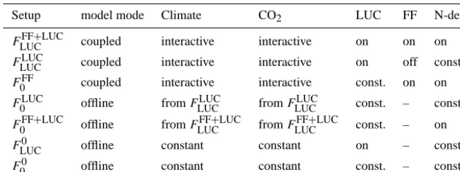
Table 1.Model setups.Fis the simulated total net flux of C from the terrestrial biosphere to the atmosphere. Subscript 0 refers to a setup where the area under use is kept constant at 1700 conditions and subscript LUC to a setup where the area under use is transiently varying
following the land cover data by Hurtt et al. (2006). Superscript LUC and FF refer to environmental changes (CO2, climate, etc.) due to
LUC forcing and non-LUC related forcing (FF) or their combination (FF+LUC). Simulations with superscript “0” are forced by constant
environmental (climate and CO2) conditions (e.g. preindustrial or modern). In coupled simulations, climate and CO2evolve interactively as
simulated by the coupled Bern3D-LPX model. The offline model mode uses either outputs from the coupled simulations or constant climate
and CO2andFis computed with the stand-alone vegetation model LPX. N-deposition (“N-dep.”) is prescribed from Lamarque et al. (2011).
Setup model mode Climate CO2 LUC FF N-dep.
FLUCFF+LUC coupled interactive interactive on on on
FLUCLUC coupled interactive interactive on off const.
F0FF coupled interactive interactive const. on on
F0LUC offline fromFLUCLUC fromFLUCLUC const. – const.
F0FF+LUC offline fromFLUCFF+LUC fromFLUCFF+LUC const. – on
FLUC0 offline constant constant on – const.
F00 offline constant constant const. – const.
4 Methods
In order to quantify the individual flux components and the discrepancy between the different quantifications of eLUC outlined in previous sections, we apply the emission-driven, coupled Bern3D-LPX Earth System Model of Intermediate Complexity as described in Stocker et al. (2013a) and the of-fline DGVM model setup where the LPX DGVM is driven in an offline mode as described in Stocker et al. (2014). Results from the offline vegetation model were also used in global C budget accountings (Le Quéré et al., 2013; Le Quéré et al., 2014, 2015), following the D3 method for estimatingeLUC therein. The model is spun up at constant boundary condi-tions representing year 1700 (CO2insolation, HYDE-based,
(Goldewijk, 2001) land use distribution from the LUH data set (Hurtt et al., 2006), and recycled 1901–1931 CRU TS 2.1 climate (Mitchell and Jones, 2005)). Model drift is absent af-ter the spin-up. During the transient simulation (1700–2100), climate is simulated by adding an anomaly pattern, scaled by global mean temperature change relative to 1700, to the con-tinuously recycled CRU climatology (temperature, precipita-tion, cloud cover). This implies that unforced variability is identical in all simulations. We focus on results after 1800 but chose an early start of the transient simulation (1700) in order to minimise effects of the initial equilibrium assump-tion for LUC-related fluxes. For the historical period and the future “business-as-usual” scenario (RCP8.5), we apply CMIP5 standard inputs (Taylor et al., 2012). Land use change is simulated following the Generated Transitions Method, in-cluding shifting cultivation-type agriculture and wood har-vesting, as described in Stocker et al. (2014). In contrast to the previous studies by Stocker et al. (2013a) and Stocker et al. (2014), we apply the model at a coarser spatial reso-lution (2.5◦×3.75◦, instead of 1◦×1◦). This has negligible effects (see Sect. 5). LUC-related CO2emissions are
calcu-lated as the difference in the land-atmosphere CO2exchange
flux between the simulation with and without LUC using Eq. (2) for the bookkeeping, Eq. (4) for the coupled, and Eq. (3) for the offline setup. In the coupled ESM setup, at-mospheric CO2 concentrations and climate evolve
interac-tively in response to the respective forcings. In the offline model setup following the D3 method, we directly prescribe climate fields and CO2concentrations to the vegetation
com-ponent (LPX model). In this case, climate and CO2are taken
from the output of the coupled ESM simulation, driven by FF and LUC (FLUCFF+LUC) and are prescribed to both offline simulations, with and without LUC. This corresponds con-ceptually to the common setup chosen for D3-type simula-tions, but instead of prescribing CO2and climate from
ob-servations (which is the result of FF and LUC as well), we prescribe it from the coupled model output here in order to exclude differences in forcings between the coupled (E2) and offline (D3) setups, and to focus on differences in computed emissions implied by the different definitions.
The model is run in a set of simulations (see Ta-ble 1) that allows us to disentangle flux components eRSS and eLFB and to assess the additivity assumption (1fFF+LUC=1fFF+1fLUC+δ). Using the description of decomposed fluxes given in Table 2 and the definition of eRSS in Eq. (7), the replaced sinks/sources flux component can be derived from simulations described in Table 1 as
eRSS=FLUCFF+LUC−FLUCLUC−F0FF
+(A0−1A)δund+1Aδdis. (15)
un-Year
Land−atmosphere
flux
[GtC
yr
]
−
1
1800 1850 1900 1950 2000 2050 2100
0.0 0.5 1.0 1.5 2.0 2.5 3.0
RCP8.5
eLUCD3: total emissions from offline DGVM
eLUCD1−PI: primary emissions − preindustrial background
eLUCD1−PD: primary emissions − present−day background
eLUCE2: total emissions from coupled ESM
(a)
Year
∆
Land−atmosphere
flux
[GtC
yr
]
−
1
1800 1850 1900 1950 2000 2050 2100
−1.0 −0.5 0.0 0.5 1.0 1.5 2.0 2.5
RCP8.5
eLUCD3 − eLUCD1
eLUCE2 − eLUCD1
eLUCD1−PD − eLUCD1−PI
(b)
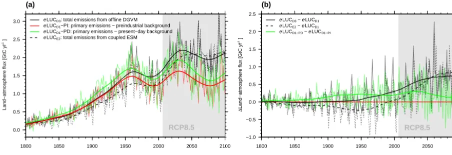
Figure 2.(a) Annual land use change emissions as quantified following different methods. (b) Difference of differenteLUC definitions
relative toeLUCdI, quantified under preindustrial boundary conditions. Total emissions derived from an offline, concentration-driven DGVM
setup (D3 method) are given by black solid lines. Total emissions derived from a coupled, emission-driven ESM setup (E2 method) are given by black dashed lines. Primary emissions are given by coloured lines under constant pre-industrial (red) and constant present-day (green)
environmental conditions (climate, CO2, N deposition). Time series are calculated following Eqs. (2)–(4), whereFis the global total
land-atmosphere CO2flux in the respective simulation. Bold lines are splines of annual emissions given by thin lines. Results are from simulations
following CMIP5 model inputs (historical until 2005, RCP8.5 until 2099).
Table 2.Flux decomposition for model setups described in Table 1.A0is land area at the reference state,1Ais the area of land converted
relative to the reference state.1fundand1fdisare the fluxes on unconverted and converted land induced by environmental change. The
underlying driver of environmental change is given by the superscripts.f0is the flux due to direct impacts of land conversion, not including
effects of environmental change.F00is zero except for the flux arising from unforced climate variability. The component fluxA01fundLUC
has not been named explicitly. Synergy terms are ignored in this table. Note that fluxesFgenerally refer to global totals for a given point in
timet. Thus, for exampleF0FF(t)= R
x,y
A0(x, y)1fundFF(x, y, t) dxdy. For simplicity, we have dropped the time and space dimensions.
Setup Decomposed flux Component fluxes
FLUCFF+LUC (A0−1A)1fundFF+LUC+1A f0+1A 1fdisFF+LUC ePS+eLUC0+eRSS+eLFB FLUCLUC (A0−1A)1fundLUC+1A f0+1A 1fdisLUC eLUC0+eLFB
F0FF A01fundFF ePS
F0LUC A01fundLUC A01fundLUC
F0FF+LUC A01fundFF+LUC ePS+A01fundLUC
FLUC0 1A f0 eLUC0
F00 ∼0 ∼0
forced variability, as neither LUC nor changing environmen-tal conditions are acting. Alternatively,eRSS can also be de-rived as (FLUCFF+LUC−F0FF+LUC)−(FLUCLUC−F0LUC), which is formally identical to Eq. (15), assuming additivity of the FF and LUC forcings. Analogously, the land use feedback flux can be derived as
eLFB=FLUCLUC−FLUC0 . (16)
Also this can be understood intuitively.eLFB represents the total land-atmosphere flux in a world with LUC (but with-out fossil fuel emissions),FLUCLUC, minus the direct effects of LUC,FLUC0 . In other words, it represents the secondary flux caused by LUC alone. Again, alternativelyeLFB can be
de-rived asFLUCFF+LUC−FLUCFF , which is identical to Eq. (16), ex-cept for synergy effects.
5 Results
Figure 1 reveals that global fluxes due to FF and due to LUC forcing alone combine in an almost perfectly addi-tive fashion to the flux induced by the combined effect of FF and LUC up to present and discernible deviations (δ) emerge only in a future scenario of continuously rising CO2
assump-Table 3.Cumulative emissions (GtC) over historical and future
pe-riod for different methods (eLUCD1,eLUCD3,eLUCE2) and
com-ponent fluxes (eRSS,eLFB).eLUCD1-PI andeLUCD1-PD refer are
quantified under preindustrial (PI) and present-day (PD) environ-mental conditions.
1850–2004 2005–2099
eLUCD1-PI 152 133
eLUCD1-PD 177 153
eLUCD3 164 192
eLUCE2 133 188
eRSS 9 71
eLFB −26 −17
tion (1fFF+LUC=1fFF+1fLUC+δ) that underpins the flux component decomposition in Sect. 3.
Figure 2 illustrates annual emissions from LUC as quanti-fied from the different approaches. During the historical pe-riod, the offline quantification (D3) suggests∼23 % higher emissions than the coupled setup (E2). Cumulative emis-sions amount to 164 GtC with D3 and 133 GtC with E2 (AD 1850–2005, see Table 3). SM08 applied observational CO2 and climate in simulations used for D3. They found
slightly higher differences of D3 vs. E2 (30 % higher in their D3). Arora and Boer (2010) report a difference of∼100 % for a case where they only used CO2 concentrations from
their interactive FLUCFF+LUC to force their F0FF+LUC simula-tion. A stronger effect in this case appears plausible as the replaced sinks/sources flux due to climate and CO2effects
are generally opposing (Strassmann et al., 2008). Stocker et al. (2014) applied the same model at a 1◦×1◦ resolu-tion following the D3 and D1 methods to quantify “total” and “primary” LUC emissions. Results at the finer resolu-tion (165 GtC for “total GNT” in their Table 3) are virtually identical to the present estimate. The bookkeeping method yields cumulative historical fluxes of 152 and 177 GtC un-der preindustrial and present-day environmental conditions. Primary emissions under preindustrial and present-day back-ground exhibit largely identical temporal trends but differ in absolute magnitude. 16 % higher emissions under present-day conditions are due to generally larger C density in natu-ral (non-cropland and non-pasture) vegetation and soils sim-ulated under elevated CO2(364 ppm) and the warmer climate
(corresponding to years AD 1982–2012 in the CRU TS 3.21 data set (Mitchell and Jones, 2005)). Differences in constant environmental conditions thus have qualitatively the same ef-fect as uncertainty in C stocks on natural and agricultural land. I.e.eLUCdI scales linearly with simulated differences in natural and agricultural land and the trends ineLUCdI de-rived under preindustrial and present-day environmental con-ditions are identical, but markedly different from trends in eLUCdIII andeLUCeII.
Cumulative historical emissions following the D1 method under preindustrial (present-day) conditions are 14 % (33 %)
Year
Land−atmosphere
flux
[GtC
yr
]
−
1
1800 1850 1900 1950 2000 2050 2100
−1 0 1 2 3
RCP8.5 eLUCE2: total emissions
eLUC0: primary emissions
eLFB: LUC feedback flux
eRSS: replaced sources/sinks emissions (eLUCE2−eLUCD3)
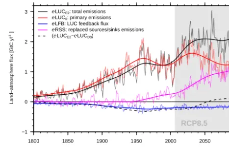
Figure 3.Flux components of land use change emissions. Total emissions as derived from an emission-driven, coupled ESM setup (E2 method), and calculated with Eq. (4), are given by the black lines. Primary emissions under preindustrial boundary conditions are given by red lines. These correspond to curves in Fig. 2. The
replaced sinks/sources flux (eRSS) and the land use change
feed-back flux (eLFB) are given by magenta and blue lines, respectively.
The difference between total emissions quantified by D3 method (see black solid line in Fig. 2) and E2 method is given by the black dashed line. Time series are calculated following Eqs. (2), (4), (15), and (16). Bold lines are splines of annual emissions given by thin lines. Results are from simulations following CMIP5 model inputs (historical until 2005, RCP8.5 until 2099).
higher than suggested by the E2 method. These differences are substantial and are on the order of the model range as presented in intercomparison studies (Sitch et al., 2008; Le Quéré et al., 2015) or on the order of effects of account-ing for wood harvest and shiftaccount-ing cultivation (Stocker et al., 2014). For the future period (AD 2006–2099) following RCP8.5, cumulative emissions (2004–2099) for the D3 and E2 method are on the same order (192 and 188 GtC), but con-siderably higher than for the D1 method (133 and 153 GtC under preindustrial and present-day conditions). Differences with respect to the relative increase from present-day emis-sion levels (average over 1995–2004) to projected levels in the last decade of the 21st century are even larger. Following the D1 method, the increase is 22 % (34 %) when holding conditions constant at preindustrial (present-day) levels. Due to different inclusion of secondary fluxes, the projected in-crease following the D3 method is 67 and 121 % following E2.
magni-−30000 −4000 −3000 −2000 −1000 0 1000 2000 3000 4000 30000
lon
lat
∆ fund
FF+LUC
lon
lat
∆ fdis
FF+LUC
−5000 −4000 −3000 −2000 −1000 0 1000 2000 3000 4000 12000
−11000 −4000 −3000 −2000 −1000 0 1000 2000 3000 4000 30000
lat
∆ fund
FF+LUC− ∆
fdis
FF+LUC
lat
Non−linearity:
∆ fund
FF+ ∆
fund
LUC− ∆
fund
FF+LUC
10000 −800 −600 −400 −200 0 200 400 600 800 13000
(a) (b)
(c) (d)
Figure 4.Top row panels: cumulative atmosphere-land C flux (kgC m−2) induced by environmental change from 1700 to 2100 on undis-turbed (a) and disundis-turbed land (b; mean of cropland and pasture, weighted by respective area shares). Here, “disundis-turbed” is approximated by cropland and pasture area (small at 1700), and “undisturbed” by natural area. The period 2005–2100 follows the RCP8.5 scenario. Climate and CO2are prescribed from the outputs of the coupled simulation (offline simulationF0FF+LUCuses outputs fromFLUCFF+LUC). (c)
Differ-ence of flux occurring on undisturbed and disturbed landfundFF+LUC−fdisFF+LUC. (d) Spatial distribution of synergy effects, cumulative in year 2100. Its global total over time is expressed also in Fig. 1 (difference between black and red curves).
tude, hence total (eLUCeII) and primary emissions (eLUCo) are at approximately the same level. In RCP8.5, atmospheric CO2and temperatures continue to grow, while land
conver-sion rates and primary emisconver-sions are stabilised. As a result eLFB is stabilised, while eRSS continues to increase and contributes∼50 % to total emissions in 2100. This explains the different trends in “total” (based on E2 and D3) versus primary emissions.
The difference betweeneLUCeII andeLUCdIII is of ap-proximately the same magnitude aseLFB , although slightly smaller, and exhibits a trend that is closely matched byeLFB until roughly AD 2030 (see dashed line in Fig. 3). This is expected as the difference, derived in Eq. (13), is equal toA0(1fundLUC+δund), and thus resembles the definition of eLFB (see Eq. 8).
Secondary emissions are determined by the magnitude of C sinks and sources induced by environmental change, occurring differently on disturbed (agricultural) and undis-turbed (natural) land. Figure 4 reveals that the C sink capac-ity on natural land under rising CO2and a changing climate
(year 2100, RCP8.5) is greatest in semi-arid regions of the Tropics and Subtropics and along the boreal treeline. In con-trast, agricultural land at low latitudes acts as a net C source under environmental change and a net sink at high latitudes. The difference between the sink strength on natural and
agri-cultural land is related to theeRSS component flux and re-veals that the Tropics are the most efficient potential C sinks. Interestingly, at high latitudes, agricultural vegetation is an even more efficient C sink than natural vegetation. Figure 4 also provides information about the spatial distribution of synergy effects from the combination of the FF and LUC forcings, corresponding to the differences between the red and the black curves in Fig. 1 in year 2100. The sum of in-dividual effects is greater than their combination in almost all vegetated areas, but most pronounced along the transition zone between forest and open woodland. Opposite effects are simulated in individual gridcells and are likely related to the threshold-behaviour of the dominant vegetation type.
6 Discussion
These differences stem from the implicit inclusion of sec-ondary flux components. As we have pointed out, secsec-ondary fluxes derived from offline vegetation model setups are con-ceptually not identical to what is commonly referred to as the replaced sinks/sources flux or the land use feedback, nor the sum of the two.
Land use change is a substantial driver of the observed CO2increase and has contributed about 25 % to total
anthro-pogenic CO2emissions for the period 1870–2014 (Le Quéré
et al., 2015). Current (2004–2013) emission levels are 0.9±0.5 GtC yr−1(Le Quéré et al., 2015). Reducing emis-sions from deforestation and forest degradation is now an im-portant part of international climate change mitigation efforts under the United Nation Framework Convention on Climate Change. Periodically issued synthesis reports by the IPCC (Ciais et al., 2013), annually updated CO2 flux
quantifica-tions by the Global Carbon Project (Le Quéré et al., 2015), as well as multi-model intercomparison projects (CMIP5, 2009; CMIP6, 2014; TRENDY, 2015) provide valuable in-formation on LUC CO2emissions. However, values derived
from different approaches are commonly presented alongside and respective uncertainty ranges partly stem from implicit methodological differences. The lack of a standard method-ological protocol for LUC emission estimates and the inclu-sion of secondary fluxes also obscures the scientific interpre-tation of model results and their comparison with observa-tional data. Below, we outline two different perspectives on what “emissions from LUC” may represent.
6.1 Carbon budget accounting
On local to regional scales, the land C budget on natural (or weakly managed) land is derived from forest inventory data (Pan et al., 2011), net ecosystem exchange estimates from eddy flux towers (Valentini et al., 2000; Friend et al., 2007), growth assessments from tree ring data, satellite data (Bac-cini et al., 2012; Harris et al., 2012), and atmospheric inver-sions of the CO2distribution using transport models (Gatti
et al., 2014). As pointed out also by Houghton (2013) and PG14, it is in general not possible to disentangle to which extent such observation-based estimates of the local net air-land C flux are driven by environmental change induced by fossil fuel combustion or by remote LUC. Fossil fuel emis-sion estimates do not, by definition, include any such sec-ondary effects.eLUC estimates including theeLFB compo-nent are thus conceptually inconsistent with reported values for fossil fuel emissions. Similarly, comparingeLUC quan-tifications that includeeRSS with up-scaled local-to-regional scale observation-based information is confounded by this virtual, because not realised, flux component.
This is relevant for continental-to-global scale C budget accounting, where CO2 exchange fluxes between the
ma-jor reservoirs (ocean, atmosphere, land, fossil fuel reserves) and the airborne fraction of anthropogenic CO2 emissions
are quantified (Canadell et al., 2007; Le Quere et al., 2009;
$nnual flux (GtC yr−1
)
−1.0 −0.5 0.0 0.5 1.0
eLUCE2
eLUCD3
eLUCD1
,mplied sink from E2
,mplied sink from D3
,mplied sink from D1
eRSS
eLFB
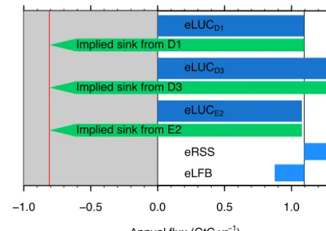
Figure 5.Land use change emissions (eLUC, dark blue bars) cal-culated from different methodologies and their implied residual
ter-restrial C sink (annual flux in GtC yr−1, mean over 1996–2005).
The total terrestrial C balance is constrained by atmospheric
mea-surements and is−0.8 GtC yr−1(mean over 1996–2005, (Le Quéré
et al., 2014), left vertical line). It is independent ofeLUC estimates. The residual terrestrial C sink (green arrow) is defined as the
differ-ence ofeLUC and the total terrestrial C balance. Depending on the
definition ofeLUC, the residual C sink is affected by inclusion of
secondary fluxes (light blue bars,eRSS andeLFB) intoeLUC.
Knorr, 2009; Ballantyne et al., 2012; Le Quéré et al., 2015). By definition, estimates foreLUC directly translate into the magnitude of the implied residual terrestrial C sink (see Fig. 5) and the airborne fraction. Inclusion of secondary LUC fluxes thus determines where the system boundaries be-tweeneLUC and the residual terrestrial sink are drawn. The D3 method ascribes replaced sinks/sources (eRSS) toeLUC. This implies that the residual terrestrial sink represents a flux occurring in a hypothetical state before land conversion. This may be misleading in view of the actual reduction of land C sinks due to the reduction of natural vegetation. This reduc-tion of the residual sink due to the replacement of natural by agricultural vegetation is only captured when basing its quantification on D1-typeeLUC estimates.
Processes determining primary emissions are directly ob-servable (i.e. C stocks in vegetation and soils, C loss dur-ing deforestation, fate of product pools, soil C evolution af-ter conversion). Such information may be used to benchmark simulatedeLUCdI. As discussed by Houghton (2013), sep-arating environmental effects from management effects (di-rect effects from LUC) also serves to lower uncertainty in eLUC estimates as it excludes effects of CO2 fertilisation
Our results also demonstrated the differences in eLUCdI implied by prescribing preindustrial versus present-day en-vironmental conditions (see Fig. 2). It may be argued that prescribing present-day conditions allows best comparabil-ity with bookkeeping estimates where observational data of C density in natural and agricultural land are used, that inherently represents conditions of the recent past. How-ever, we note that total terrestrial C storage is 1775, 1838, and 1982 GtC in our simulations for FLUC0−PI,FLUCFF+LUC, and FLUC0−PD (mean over years 2000–2004; superscript “0−PI” [“0−PD”] refers to constant preindustrial [present-day] en-vironmental conditions). I.e. the case where C stocks are re-sponding to transient changes in CO2and climate (FLUCFF+LUC
– the closest analogue to what observational data represent) is farther from its equilibrium to be attained under present-day conditions than its equilibrium under preindustrial con-ditions. In other words, quantifyingeLUCdI under preindus-trial conditions is a viable and pragmatic solution.
Adopting the D1 method for benchmarking, model-intercomparison studies and syntheses based on multiple methods has the critical practical advantage of being the “least common denominator” that can be followed using empirically based bookkeeping methods, offline vegetation models, as well as Earth System Models. Quantification of eLUCdI simply requires a preindustrial control simulation (no forcings, constant environmental conditions) which is al-ready part of the CMIP6 DECK simulations (CMIP6, 2014), and one additional run with transient LUC while environ-mental conditions are held constant at preindustrial levels (see Sect. 4). This could be achieved by Earth System Models without computationally demanding coupled model setups involving interactive atmosphere and ocean, but using pre-scribed preindustrial climate and CO2and their land models
in a stand-alone mode instead. Serving as an “entry card” for future model intercomparisons, this would guarantee conti-nuity and comparability between model development cycles and periodically repeated syntheses.
6.2 LUC in the Earth system
LUC effects on climate and the Earth system are not fully captured by their direct (primary) CO2emissions. Vegetation
cover change also affects the local surface energy and wa-ter balances (biogeophysical effects) and emissions of other greenhouse gases. Deforestation by purposely set fires is as-sociated with emissions of a range of radiatively active com-pounds (e.g. CH4, CO, NOx), wetland management may
have strong effects on CH4emissions, and the application of
mineral fertiliser and manure on agricultural land increases soil N2O emissions and sets in motion a cascade of
detri-mental environdetri-mental effects (Galloway et al., 2003), many of which directly or indirectly affect climate (Erisman et al., 2011).
Apart from these direct effects where LUC can be re-garded as a forcing acting upon the Earth system, LUC also
modifies the land response to external forcings. E.g. the re-placement of woody vegetation with crops reduces the CO2
-driven fertilisation sink. Thus, LUC affects the strength of the land-climate feedback (Stocker et al., 2013a). Further-more, primary LUC emissions induce a secondary C uptake flux as a feedback to elevated CO2concentrations caused by
primary emissions. These feedback effects are captured by the LUC flux componentseRSS and eLFB. Coupled Earth System Models featuring an active C cycle require a prein-dustrial control simulation and a fossil C emission-driven simulation over the industrial period where transient LUC and other climate and environmental forcings are activated to quantify the sum of primary and secondary land use C emissions (method E2). Such an emission-driven, land use-enabled simulation may become part of the CMIP6 proto-col. Additional simulations are required to quantify individ-ual components separately (see Table 2).
The results presented here demonstrate the importance of secondary fluxes under slowing land conversion rates and continuously increasing CO2. In RCP8.5,eRSS is set to
in-crease to±1 GtC yr−1and make up around half ofeLUCeII by the end of the 21st century. Hence, in order to capture the overall effect of LUC on the terrestrial C cycle feedback, these must be accounted for. However, we recommend to ac-count for the effect of secondary LUC-related fluxes in global C budget assessments as an anthropogenic modification of the terrestrial C sink. We emphasize that offline vegetation model setups are not capable of separatingeRSS andeLFB as defined here.
7 Conclusions
Estimates of CO2 emissions from land use are essential to
Acknowledgements. This study received support from the Swiss National Science Foundation (SNF), the iTREE project (CR-SII3 136295) of the SNF, and by the European Commission through the FP7 projects CARBOCHANGE (grant no. 264879) and EMBRACE (grant no. 282672). We thank Raphael Roth for help with coupled simulations.
Edited by: C. Reick
References
Arora, V. K. and Boer, G. J.: Uncertainties in the 20th century carbon budget associated with land use change, Global Change Biol., 16, 3327–3348, doi:10.1111/j.1365-2486.2010.02202.x, 2010.
Baccini, A., Goetz, S. J., Walker, W. S., Laporte, N. T., Sun, M., Sulla-Menashe, D., Hackler, J., Beck, P. S. A., Dubayah, R., Friedl, M. A., Samanta, S., and Houghton, R. A.: Esti-mated carbon dioxide emissions from tropical deforestation im-proved by carbon-density maps, Nat. Clim. Change, 2, 182–185, doi:10.1038/nclimate1354, 2012.
Ballantyne, A. P., Alden, C. B., Miller, J. B., Tans, P. P., and White, J. W. C.: Increase in observed net carbon dioxide uptake by land and oceans during the past 50 years, Nature, 488, 70–72, doi:10.1038/nature11299, 2012.
Canadell, J. G., Le Quere, C., Raupach, M. R., Field, C. B., Buiten-huis, E. T., Ciais, P., Conway, T. J., Gillett, N. P., Houghton, R. A., and Marland, G.: Contributions to accelerating
atmo-spheric CO2 growth from economic activity, carbon intensity,
and efficiency of natural sinks, P. Natl. Acad. Sci., 104, 18866– 18870, doi:10.1073/pnas.0702737104, 2007.
Ciais, P., Sabine, C., Bala, G., Bopp, L., Brovkin, V., Canadell, J., A., C., DeFries, R., J., G., Heimann, M., Jones, C., Le Quéré, C., Myneni, R., S., P., and Thornton, P.: Carbon and Other Biogeo-chemical Cycles, in: Climate Change 2013: The Physical Science Basis, in: Working Group I Contribution to the Fifth Assessment Report of the Intergovernmental Panel on Climate Change, edited by: Stocker, T., Qin, D., Plattner, G.-K., Tignor, M., Allen, S., Boschung, J., Nauels, A., Xia, Y., Bex, V., and Midgley, P., Cam-bridge University Press, 571–658, 2013.
CMIP5: CMIP5 Coupled Model Intercomparison Project, avail-able at: http://cmip-pcmdi.llnl.gov/index.html (last access: 27 November 2011), 2009.
CMIP6: CMIP Phase 6, available at: http://www.wcrp-climate.org/ wgcm-cmip/wgcm-cmip6 (last access: 19 February 2015), 2014. Erisman, J. W., Galloway, J., Seitzinger, S., Bleeker, A., and Butterbach-Bahl, K.: Reactive nitrogen in the environment and its effect on climate change, Curr. Opin. Environ. Sustain., 3, 281–290, doi:10.1016/j.cosust.2011.08.012, 2011.
Friedlingstein, P., Cox, P., Betts, R., Bopp, L., von Bloh, W., Brovkin, V., Cadule, P., Doney, S., Eby, M., Fung, I., Bala, G., John, J., Jones, C., Joos, F., Kato, T., Kawamiya, M., Knorr, W., Lindsay, K., Matthews, H. D., Raddatz, T., Rayner, P., Reick, C., Roeckner, E., Schnitzler, K. G., Schnur, R., Strassmann, K., Weaver, A. J., Yoshikawa, C., and Zeng, N.: Climate-Carbon Cycle Feedback Analysis: Results from the C4MIP Model Intercomparison, J. Climate, 19, 3337–3353, doi:10.1175/JCLI3800.1, 2006.
Friend, A. D., Arneth, A., Kian, N. Y., Lomas, M., Ogee, J., Ro-denbeck, C., Running, S. W., Santaren, J.-D., Sitch, S., Viovy, N., Woodward, I. F., and Zaehle, S.: FLUXNET and modelling the global carbon cycle, Global Change Biol., 13, 610–633, doi:10.1111/j.1365-2486.2006.01223.x, 2007.
Galloway, J., Aber, J., Erisman, J., Seitzinger, S., Howarth,
R., Cowling, E., and Cosby, B.: The nitrogen
cas-cade, Bioscience, 53, 341–356,
doi:10.1641/0006-3568(2003)053[0341:TNC]2.0.CO;2, 2003.
Gasser, T. and Ciais, P.: A theoretical framework for the net
land-to-atmosphere CO2flux and its implications in the definition of
“emissions from land-use change”, Earth Syst. Dynam., 4, 171– 186, doi:10.5194/esd-4-171-2013, 2013.
Gatti, L. V., Gloor, M., Miller, J. B., Doughty, C. E., Malhi, Y., Domingues, L. G., Basso, L. S., Martinewski, A., Correia, C. S. C., Borges, V. F., Freitas, S., Braz, R., Anderson, L. O., Rocha, H., Grace, J., Phillips, O. L., and Lloyd, J.: Drought sensitivity of Amazonian carbon balance revealed by atmospheric measure-ments, Nature, 506, 76–80, doi:10.1038/nature12957, 2014. Gitz, V. and Ciais, P.: Amplification effect of changes in land
use and concentration of atmospheric CO2, Comptes Rendus
Geosci., 335, 1179–1198, 2003.
Gitz, V. and Ciais, P.: Amplifying effects of land-use change on
fu-ture atmospheric CO2levels, Global Biogeochem. Cy., 17, 1024,
doi:10.1029/2002GB001963, 2003.
Goldewijk, K. K.: Estimating global land use change over the past 300 years: the HYDE database, Global Biogeochem. Cy., 15, 417–434, 2001.
Harris, N. L., Brown, S., Hagen, S. C., Saatchi, S. S., Petrova, S., Salas, W., Hansen, M. C., Potapov, P. V., and Lotsch, A.: Baseline Map of Carbon Emissions from Deforestation in Tropical Re-gions, Science, 336, 1573–1576, doi:10.1126/science.1217962, 2012.
Houghton, R. A.: The annual net flux of carbon to the atmosphere from changes in land use 1850–1990, Tellus B, 51, 298–313, 1999.
Houghton, R. A.: Keeping management effects separate from environmental effects in terrestrial carbon accounting, Global Change Biol., 19, 2609–2612, 2013.
Houghton, R. A., Hobbie, J. E., Melillo, J. M., Moore, B., Peterson, B. J., Shaver, G. R., and Woodwell, G. M.: Changes in the carbon content of terrestrial biota and soils between 1860 and 1980 - a
net release of CO2to the atmosphere, Ecol. Monogr., 53, 235–
262, 1983.
Houghton, R. A., House, J. I., Pongratz, J., van der Werf, G. R., De-Fries, R. S., Hansen, M. C., Le Quéré, C., and Ramankutty, N.: Carbon emissions from land use and land-cover change, Biogeo-sciences, 9, 5125–5142, doi:10.5194/bg-9-5125-2012, 2012. Hurtt, G. C., Frolking, S., Fearon, M. G., Moore, B.,
Shevli-akova, E., Malyshev, S., Pacala, S. W., and Houghton, R. A.: The underpinnings of land-use history: three centuries of global gridded land-use transitions, wood-harvest activity, and result-ing secondary lands, Global Change Biol., 12, 1208–1229, doi:10.1111/j.1365-2486.2006.01150.x, 2006.
Jones, C., Robertson, E., Arora, V., Friedlingstein, P., Shevliakova, E., Bopp, L., Brovkin, V., Hajima, T., Kato, E., Kawamiya, M., Liddicoat, S., Lindsay, K., Reick, C. H., Roelandt, C., Segschneider, J., and Tjiputra, J.: Twenty-First-Century
Earth System Models under Four Representative Concentration Pathways, J. Climate, 26, 4398–4413, doi:10.1175/JCLI-D-12-00554.1, 2013.
Joos, F., Prentice, I. C., Sitch, S., Meyer, R., Hooss, G., Plattner, G.-K., Gerber, S., and Hasselmann, K.: Global warming feed-backs on terrestrial carbon uptake under the Intergovernmen-tal Panel on Climate Change (IPCC) emission scenarios, Global Biogeochem. Cy., 15, 891–907, 2001.
Knorr, W.: Is the airborne fraction of anthropogenic CO2
emissions increasing?, Geophys. Res. Lett., 36, L21710, doi:10.1029/2009GL040613, 2009.
Lamarque, J.-F., Kyle, G. P., Meinshausen, M., Riahi, K., Smith, S. J., van Vuuren, D. P., Conley, A. J., and Vitt, F.: Global and regional evolution of short-lived radiatively-active gases and aerosols in the Representative Concentration Pathways, Climatic Change, 109, 191–212, doi:10.1007/s10584-011-0155-0, 2011. Le Quere, C., Raupach, M. R., Canadell, J. G., and Marland, G.,
Bopp, L., Ciais, P., Conway, T. J., Doney, S. C., Feely, R. A., Fos-ter, P., Friedlingstein, P.,Gurney, K., Houghton, R. A., House, J. I., Huntingford, C., Levy, P. E., Lomas, M. R., Majkut, J., Metzl, N., Ometto, J. P., Peters, G. P., Prentice, I. C., Randerson, J. T., Running, S. W., Sarmiento, J. L., Schuster, U., Sitch, S., Taka-hashi, T., Viovy, N., van der Werf, G. R., and Woodward, F. I.: Trends in the sources and sinks of carbon dioxide, Nat. Geosci., 2, 831–836, doi:10.1038/ngeo689, 2009.
Le Quéré, C., Andres, R. J., Boden, T., Conway, T., Houghton, R. A., House, J. I., Marland, G., Peters, G. P., van der Werf, G. R., Ahlström, A., Andrew, R. M., Bopp, L., Canadell, J. G., Ciais, P., Doney, S. C., Enright, C., Friedlingstein, P., Hunting-ford, C., Jain, A. K., Jourdain, C., Kato, E., Keeling, R. F., Klein Goldewijk, K., Levis, S., Levy, P., Lomas, M., Poulter, B., Rau-pach, M. R., Schwinger, J., Sitch, S., Stocker, B. D., Viovy, N., Zaehle, S., and Zeng, N.: The global carbon budget 1959–2011, Earth Syst. Sci. Data, 5, 165–185, doi:10.5194/essd-5-165-2013, 2013.
Le Quéré, C., Peters, G. P., Andres, R. J., Andrew, R. M., Boden, T. A., Ciais, P., Friedlingstein, P., Houghton, R. A., Marland, G., Moriarty, R., Sitch, S., Tans, P., Arneth, A., Arvanitis, A., Bakker, D. C. E., Bopp, L., Canadell, J. G., Chini, L. P., Doney, S. C., Harper, A., Harris, I., House, J. I., Jain, A. K., Jones, S. D., Kato, E., Keeling, R. F., Klein Goldewijk, K., Körtzinger, A., Koven, C., Lefèvre, N., Maignan, F., Omar, A., Ono, T., Park, G.-H., Pfeil, B., Poulter, B., Raupach, M. R., Regnier, P., Rödenbeck, C., Saito, S., Schwinger, J., Segschneider, J., Stocker, B. D., Taka-hashi, T., Tilbrook, B., van Heuven, S., Viovy, N., Wanninkhof, R., Wiltshire, A., and Zaehle, S.: Global carbon budget 2013, Earth Syst. Sci. Data, 6, 235–263, doi:10.5194/essd-6-235-2014, 2014.
Le Quéré, C., Moriarty, R., Andrew, R. M., Peters, G. P., Ciais, P., Friedlingstein, P., Jones, S. D., Sitch, S., Tans, P., Arneth, A., Boden, T. A., Bopp, L., Bozec, Y., Canadell, J. G., Chini, L. P., Chevallier, F., Cosca, C. E., Harris, I., Hoppema, M., Houghton, R. A., House, J. I., Jain, A. K., Johannessen, T., Kato, E., Keel-ing, R. F., Kitidis, V., Klein Goldewijk, K., Koven, C., Landa, C. S., Landschützer, P., Lenton, A., Lima, I. D., Marland, G., Mathis, J. T., Metzl, N., Nojiri, Y., Olsen, A., Ono, T., Peng, S., Peters, W., Pfeil, B., Poulter, B., Raupach, M. R., Regnier, P., Rö-denbeck, C., Saito, S., Salisbury, J. E., Schuster, U., Schwinger, J., Séférian, R., Segschneider, J., Steinhoff, T., Stocker, B. D.,
Sutton, A. J., Takahashi, T., Tilbrook, B., van der Werf, G. R., Viovy, N., Wang, Y.-P., Wanninkhof, R., Wiltshire, A., and Zeng, N.: Global carbon budget 2014, Earth Syst. Sci. Data, 7, 47–85, doi:10.5194/essd-7-47-2015, 2015.
McGuire, A. D., Sitch, S., Clein, J. S., Dargaville, R., Esser, G., Foley, J., Heimann, M., Joos, F., Kaplan, J., Kicklighter, D. W., Meier, R. A., Melillo, J. M., Moore III, B., Prentice, I. C., Ra-mankutty, N., Reichenau, T., Schloss, A., Tian, H., Williams, L. J., and Wittenberg, U.: Carbon balance of the terrestrial
biosphere in the twentieth century: Analyses of CO2, climate
and land use effects with four process-based ecosystem models, Global Biogeochem. Cy., 15, 183–206, 2001.
Mitchell, T. D. and Jones, P. D.: An improved method of con-structing a database of monthly climate observations and as-sociated high-resolution grids, Int. J. Climatol., 25, 693–712, doi:10.1002/joc.1181, 2005.
Pan, Y., Birdsey, R. A., Fang, J., Houghton, R., Kauppi, P. E., Kurz, W. A., Phillips, O. L., Shvidenko, A., Lewis, S. L., Canadell, J. G., Ciais, P., Jackson, R. B., Pacala, S. W., McGuire, A. D., Piao, S., Rautiainen, A., Sitch, S., and Hayes, D.: A Large and Persistent Carbon Sink in the World’s Forests, Science, 333, 988– 993, doi:10.1126/science.1201609, 2011.
Pongratz, J., Reick, C. H., Raddatz, T., and Claussen, M.: Ef-fects of anthropogenic land cover change on the carbon cycle of the last millennium, Global Biogeochem. Cy., 23, GB4001+, doi:10.1029/2009GB003488, 2009.
Pongratz, J., Reick, C. H., Houghton, R. A., and House, J. I.: Ter-minology as a key uncertainty in net land use and land cover change carbon flux estimates, Earth Syst. Dynam., 5, 177–195, doi:10.5194/esd-5-177-2014, 2014.
Sitch, S., Huntingford, C., Gedney, N., Levy, P. E., Lomas, M., Piao, S. L., Betts, R., Ciais, P., Cox, P., Friedlingstein, P., Jones, C. D., Prentice, I. C., and Woodward, F. I.: Evaluation of the terres-trial carbon cycle, future plant geography and climate-carbon cycle feedbacks using five Dynamic Global Vegetation Mod-els (DGVMs), Global Change Biol., 14, 2015–2039, 2008. Stein, U. and Alpert, P.: Factor Separation in Numerical
Sim-ulations, J. Atmos. Sci., 50, 2107–2115, doi:10.1175/1520-0469(1993)050<2107:FSINS>2.0.CO;2, 1993.
Stocker, B. D., Strassmann, K., and Joos, F.: Sensitivity of Holocene
atmospheric CO2and the modern carbon budget to early human
land use: analyses with a process-based model, Biogeosciences, 8, 69–88, doi:10.5194/bg-8-69-2011, 2011.
Stocker, B. D., Roth, R., Joos, F., Spahni, R., Steinacher, M., Za-ehle, S., Bouwman, L., Xu-Ri, X.-R., and Prentice, I. C.: Mul-tiple greenhouse-gas feedbacks from the land biosphere under future climate change scenarios, Nat. Clim. Change, 3, 666–672, 2013a.
Stocker, B. D., Feissli, F., Strassmann, K., Spahni, R., and Joos, F.: Past and future carbon fluxes from land use change, shifting cultivation and wood harvest, Tellus B, 66, 23188, doi:10.3402/tellusb.v66.23188, 2014.
Strassmann, K. M., Joos, F., and Fischer, G.: Simulating ef-fects of land use changes on carbon fluxes: past contributions
to atmospheric CO2 increases and future commitments due
to losses of terrestrial sink capacity, Tellus B, 60, 583–603, doi:10.1111/j.1600-0889.2008.00340.x, 2008.
Taylor, K. E., Stouffer, R. J., and Meehl, G. A.: An overview of CMIP5 and the experiment design, B. Am. Meteorol. Soc., 93, 485–498, doi:10.1175/BAMS-D-11-00094.1, 2012.
TRENDY: TRENDY, available at: http://dgvm.ceh.ac.uk/node/21, last access: 19 February 2015.