Nonlinear Processes
in Geophysics
c
European Geophysical Society 2001
Diffusive draining and growth of eddies
S. Balasuriya1and C. K. R. T. Jones1
1Division of Applied Mathematics, Brown University, Providence RI 02912, USA Received: 31 March 2000 – Accepted: 30 November 2000
Abstract. The diffusive effect on barotropic models of
meso-scale eddies is addressed, using the Melnikov method from dynamical systems. Simple geometric criteria are obtained, which identify whether a given eddy grows or drains out, un-der a diffusive (and forcing) perturbation on a potential vor-ticity conserving flow. Qualitatively, the following are shown to be features conducive to eddy growth (and, thereby, sta-bility in a specific sense): (i) large radius of curvature of the eddy boundary, (ii) potential vorticity contours more tightly packed within the eddy than outside, (iii) acute eddy pinch-angle, (iv) small potential vorticity gradient across the eddy boundary, and (v) meridional wind forcing, which increases in the northward direction. The Melnikov approach also sug-gests how tendrils (filaments) could be formed through the breaking of the eddy boundary, as a diffusion-driven advec-tive process.
1 Eddies and their stability
Rings (or eddies) are significant oceanographic features which contribute considerably to fluid transport in the ocean. In particular, mesoscale (of the order of 100 km) rings formed near the Gulf Stream sometimes survive as coher-ent structures for periods of up to one year (Richardson, 1983). Submesoscale (of the order of 10 km ) eddies may also be long-lived, and we address both mesoscale and sub-mesoscale eddies in the present work. The observational per-sistence of such eddies has led to theoretical (Flierl, 1988; Helfrich and Send, 1988; Dewar and Gailliard, 1994; De-war and Killworth, 1995; Paldor, 1999), numerical (Helfrich and Send, 1988; Dewar and Gailliard, 1994; Dewar and Kill-worth, 1995; Dewar et al., 1999; Paldor, 1999; McWilliams et al., 1986) and experimental (Voropayev et al., 1999) analy-ses of stability. Since many results indicate that eddies would tend to be unstable, explaining their persistence remains an Correspondence to: S. Balasuriya
(sanjeeva.balasuriya@oberlin.edu)
active area of research. In this paper, we address a particular aspect of stability of such eddies, which reflects the effect of small diffusivity on the eddy boundary.
Though characterised by swirling fluid motions, eddies are often identified experimentally through Eulerian contour plots of temperature, height, salinity, or potential vorticity fields, usually obtained from two-dimensional satellite imag-ing data (for a review and pictures of contours, see Richard-son, 1983), or from numerical schemes. Since fluid motion in the upper ocean tends to remain on surfaces of constant temperature (resp. salinity, potential vorticity, etc), rotational motion results around maxima/minima points of the appro-priate scalar field, thereby forming a ‘ring’ (or vortical mo-tion) in the expected sense. Often, tendrils (or filaments) are seen to emanate from these eddies, which appear to wrap around the eddy (see Fig. 4 in the experimental paper by Voropayev et al., 1999, for example).
and Papanicolaou, 1994) senses. Bounds on the eddy dif-fusivity (Fannjiang and Papanicolaou, 1994; Biferale et al., 1995; Mezi´c et al., 1996), and descriptions of chaotic motion (Rom-Kedar and Poje, 1999; Klapper, 1992; Jones, 1994), are several features of interest. Even when not modelling flows with diffusivity, numerical methods often introduce a diffusivity in the interest of numerical stability, and, there-fore, such numerical models could also be thought of as in-cluding eddy diffusivity effects (Rogerson et al., 1999). Un-like in regular advection-diffusion equations, the scalar quan-tity here is an active (as opposed to passive) scalar, since the potential vorticity possesses a relationship to the fluid veloc-ity field (Pedlosky, 1987). In this study, we shall investigate how the dynamic process of eddy diffusivity affects the ge-ometry of eddies, using a new approach, which uses elements from dynamical systems theory (Balasuriya et al., 1998), and simple geometric arguments.
Our first focus in this paper is to obtain a relationship be-tween the growth (or decay) of such eddies, and the charac-teristics of the scalar potential vorticity field. Would it be possible, for example, to view the field, identify a particu-lar eddy, and predict its chances of survival based on simple geometric properties of the scalar field? In response to this, we are able to develop a collection of (diffusivity-driven) ge-ometric conditions for eddy growth, outlined in Sect. 5. It would be instructive to test our criteria upon available data sets with sufficient resolution. Moreover, in Sect. 7, we also obtain a qualitative condition on (small) wind forcing, which also contributes to eddy growth. ‘Growth,’ as specified in both these cases, will be defined through the enlargement of the eddy boundary; a shrinking boundary will correspond to a ‘draining’ eddy. Growing eddies have the potential of be-ing more visible, and, therefore, are expected to be the longer lasting eddies in the ocean. Draining (shrinking) eddies, on the other hand, will eventually lose their constituent water to the ambient flow, and disappear. Therefore, in a sense, our eddy growth criteria reflect a form of eddy stability in the presence of (small) eddy diffusivity and wind forcing. It must be re-emphasised that this ‘stability’ is not in the tra-ditional sense of linear stability, in which the growth rate of various modes of imposed perturbations is analysed, as in Flierl (1988); Helfrich and Send (1988); Paldor (1999); De-war and Killworth (1995); DeDe-war et al. (1999).
The analysis we follow in this study is generic, and should be applicable to any system satisfying a similar advection-diffusion partial differential equation in two dimensions (for example, in tracer mixing in hydrodynamics, or in atmo-spheric flows). In other words, we are not using a specific model for the flows; rather, we are simply assuming that the flow satisfies the appropriate dynamical equation, and pos-sesses the necessary kinematical properties of an eddy. These statements are made precise in Sect. 2. Section 3 then out-lines the Melnikov approach from dynamical systems theory, which leads to the eddy growth criteria in Sects. 5 and 7.
A secondary goal of this paper is to give a possible expla-nation for the tendrils which emanate from eddies. Numer-ical and experimental studies, even in the laboratory rather
than in the oceans, display such filaments (see Voropayev et al., 1999, for example), whose presence is certainly linked to eddy diffusivity (Robinson, 1983). Nevertheless, a geo-metric description of the process is lacking. Our analysis of the advection-diffusion process, from a dynamical systems viewpoint, affords an immediate and simple reasoning for the appearance of a tendril in a certain type of eddy, as ex-plained in Sect. 6. In this case, too, it is necessary to address the deformation of the eddy boundary, which links the two aspects of this paper.
2 Dynamics
In this section, we state the mathematical equations which need to be satisfied, and also characterise the eddy bound-ary whose deformation is of interest. Consider a two-dimensional incompressible flow which is steady in a moving frame. This hypothesis is in keeping with many Gulf Steam models (Pierrehumbert, 1991; del Castillo-Negrete and Mor-rison, 1993; Pratt et al., 1995; Balasuriya et al., 1998; Weiss and Knobloch, 1989), since the Gulf Steam is steady in a gross sense in an eastward moving frame. Let (x, y) be the eastward and northward coordinates, andψ0(x, y, t )the streamfunction of the flow. Suppose that there exists a quan-tity (which we shall call the potential vorticity)q0(x, y, t ) which is conserved following the flow. Such is afforded in barotropic models, for example, by the quantity∇2ψ0+βy, whereβis the Coriolis parameter (Pedlosky, 1987). Depend-ing on the particular outlook adopted, many alternative def-initions of potential vorticity exist (Pedlosky, 1987), but for our purposes it suffices to think ofq0(x, y, t )as any quantity which is preserved by the flow, and thereby
Dq0
Dt = ∂q0
∂t − ∂ψ0
∂y ∂q0
∂x + ∂ψ0
∂x ∂q0
∂y =0. (1)
Particle trajectories are found by solving the ordinary differ-ential equations
˙
x= −∂ψ0
∂y , y˙= ∂ψ0
∂x . (2)
Eddy
boundary
A
Fig. 1. Potential vorticity contours (q0(x, y, t0)=constant).
our definition of an eddy is in an Eulerian rather than a La-grangian sense, similar to the development in Haller and Poje (1997), who, in contrast, base their definitions on stream-function contours, and limit the analysis to adiabatic flows. We intend to discuss the possibility of the growth of the eddy, when a suitable diffusive perturbation to the dynamics of (1) is added. To do so, we must first identify the boundary of the eddy. This shall be a contour ofq0(x, y, t0)beyond which the contour structure changes from simple closed curves to something else. It is not difficult to see that, in order for this to happen topologically for a continuous functionq0, the boundary of the eddy must contain at least one saddle point ofq0(x, y, t0). In this paper, we shall only consider exactly one saddle pointA, in which case, the eddy has the struc-ture shown in Fig. 1 (see Fig. 1 of Weiss, 1994, for a similar picture generated through a kinematic isolated eddy model). The saddle pointAis a specialised point on the eddy bound-ary, and shall also be referred to as the pinch-off point. Under our present assumptions, this eddy structure would rigidly translate; no growth or shrinking can occur.
Potential vorticity conservation is, in reality, only approxi-mately satisfied for oceanic flows (Pedlosky, 1987). We shall consider the case where the flow satisfies not the dynamics of (1), but the ‘nearby’ dynamics given by
Dq Dt =
∂q ∂t −
∂ψ ∂y
∂q ∂x +
∂ψ ∂x
∂q ∂y =
h
∇2q+f (x, y, t )
i
.(3) Here,q(x, y, t )is a perturbed potential vorticity, and the cor-responding streamfunction isψ (x, y, t ). The small positive quantity governs the size of both the diffusive term∇2q and the additional forcing f (x, y, t ), and may be thought of as a reciprocal P´eclet number. In an oceanographic
con-text, the dynamics (3) models the presence of eddy diffu-sivity (averaged effect of small scale turbulence), and wind forcing, but assumes that these are both small effects in com-parison to the conservation of potential vorticity (i.e. is small). Equation (3) is an advection-diffusion equation; the potential vorticity changes with time due to advection (flow of particles which have a signature potential vorticity) and also diffusion (the slow decay of potential vorticity, indepen-dent of attachment to particles). This cannot be thought of as a linear equation since the potential vorticity is linked with the streamfunction. Assuming the barotropicβ-plane model (whereq = ∇2ψ+βy), it is possible to show that the stream-functionψis orderclose toψ0(Balasuriya, 1997). Crucial to this proof is the absence of boundaries (or being far re-moved from boundaries); if not, this closeness may worsen to O(√), as suggested by recent results from fluid mechanics (Caflisch and Sammartino, 1998). The governing equations of particle trajectories
˙
x= −∂ψ
∂y , y˙= ∂ψ
∂x, (4)
has a velocity field which is, therefore,-close to that of (2). It should be noted that the ‘steady in a moving frame’ prop-erty has been destroyed in the perturbed flow (4); it is gen-uinely unsteady. The eddy boundary now perturbs: it may enlarge (a growing eddy), decrease (a shrinking eddy), or de-velop kinks (leading to tendrils). This geometric deformation shall be analysed using a technique from dynamical systems theory called the Melnikov method.
3 Melnikov function
To use the so-called Melnikov approach, it is first necessary to identify a fixed point and an associated homoclinic trajec-tory of the unperturbed fluid trajectrajec-tory equation (2). Such exist if we consider the motion not in the(x, y)space, but in the moving coordinate frame in which the motion is steady. To be concrete, let us define new variablesξ =x−c1t and η=y−c2t, such that the flow of (2) is steady in the(ξ, η) frame (note, that in many standard oceanographic applica-tions,c2 = 0; yet we are able to address this more general case in which eddies may propagate in an arbitrary direction, incorporating, for example, the eddies described in Dewar and Gailliard, 1994). Then, sinceξ˙= ˙x−c1andη˙= ˙y−c2, we have
˙ ξ = − ∂
∂η[90(ξ, η)+c1η−c2ξ] ˙
η= ∂
∂ξ [90(ξ, η)+c1η−c2ξ]. (5)
is not difficult to show using (1) expressed in the(ξ, η) coor-dinates thatQ0(ξ, η)is functionally related to this effective streamfunction; the flow is confined to the curvesQ0(ξ, η)=
constant (or equivalently, curves where the effective stream-function is constant). An incidental observation, which shall become important later, is that the spatial derivatives∇,∇2, etc, remain invariant under the transformation from(x, y)to (ξ, η).
Now in the(ξ, η)frame, the eddy illustrated in Fig. 1 ex-ists as a steady object, and, therefore, the special pointAis, in fact, a fixed point of the flow (5). Additionally, it is a sad-dle point of theQ0scalar field, and hence,∇Q0is zero atA. With no loss of generality, we shall choose the origin(0,0) of the(ξ, η)system to be precisely at the pointA. Note the presence of a specialised trajectory of (5), which approaches the origin in forward and backwards time. This is a homo-clinic trajectory; (a branch of) the unstable manifold of the fixed point coinciding with (a branch of) its stable manifold. The stable manifold (denotedWs) is the set of points which asymptotically approaches the fixed point in forward time, while the unstable manifold (denotedWu) does so in back-ward time. The homoclinic precisely defines the eddy bound-ary, and, therefore, the growth of the eddy is affected by how this homoclinic trajectory perturbs. Now the homoclinic tra-jectory can be represented by ξ (t ),¯ η(t )¯ , parametrised by timet, as shown in Fig. 2. At each pointP (t )= ξ (t ),¯ η(t )¯ , one can draw a normalN (t )to the eddy boundary, whose di-rection is given by the vector∇Q0 ξ (t ),¯ η(t )¯ , which points either into or out of the eddy (this direction remains con-sistent on the homoclinic). This vector decays to zero as t → ±∞; i.e. as the origin is approached. We now ad-dress how the homoclinic trajectory, which forms the eddy boundary, perturbs under the dissipative perturbation given by (3).
Suppose the solution to (3) is given in terms of the moving frame coordinates by9(ξ, η, t ). An explicitt-dependence exists in this perturbed streamfunction, since the flow is no longer steady in the moving frame. However,9and90 dif-fer only byO(). The relevant particle trajectories in the moving frame are obtained through solving
˙ ξ = − ∂
∂η[9(ξ, η, t )+c1η−c2ξ] ˙
η= ∂
∂ξ [9(ξ, η, t )+c1η−c2ξ]. (6)
In contrast with the unperturbed moving frame equation (5), equation (6) has explicitt-dependence. Its phase space, then, is three-dimensional, and given by the variables(ξ, η, t ). The fixed point at the origin perturbs to a trajectory in this three-dimensional phase space, which remainsO()close to the line(ξ, η)=(0,0). The associated stable and unstable man-ifolds of this trajectory, two-dimensional in this three-dimen-sional phase-space, also persist. The proofs of these two claims follow from theoretical results from dynamical sys-tems (Hirsch et al., 1977; Fenichel, 1971). The key point, however, is that there is no reason for the stable and unsta-ble manifolds to coincide any more. Imagine that we have
(t))
u
W
s
W
η
(t),
ξ
∆
Q0 (ξ η
N(t)
A
Fig. 2. The unperturbed eddy in the(ξ, η)moving frame.
intersected the three-dimensional phase-space with a plane
{t = constant}. If unperturbed (if = 0), one obtains ex-actly the picture of Fig. 2 in each and everyt-slice. When 6= 0, on the other hand, a generic picture of the form of Fig. 3 is formed. The perturbed manifoldsWs andWu la-belled in Fig. 3 are, in reality, the intersections of the two-dimensional manifolds with thet =constant time-slice. The Melnikov approach provides a method of measuring the dis-tance between the perturbed manifolds in this time slice of the phase-space. Consider any pointP (t ) = ξ (t ),¯ η(t )¯ on the unperturbed homoclinic (sketched as a dashed curve in Fig. 3), and think of measuring the distanced(t )between the perturbed manifolds along the normalN (t )drawn atP (t ). Thisd(t )shall be a signed distance, whose sign is allocated as follows. If the vector drawn from the perturbed stable manifoldWsto the perturbed unstable manifoldWuis in the direction of∇Q0(P (t )), then a positive value is assigned; if in the opposite direction, a negative value is given. Notice that ifd(t )=0, there is an intersection between these mani-folds atP (t ), which may result in complicated mixing across the eddy boundary nearP (t )due to homoclinic tangling. It turns out thatd(t )can be expressed as
d(t )= M(t ) ∇Q0(P (t ))
+O(2), (7)
η
ξ
W A
P(t)
d(t)
u
W N(t)
s
Fig. 3. The perturbed eddy in the(ξ, η)moving frame.
theO()term is nonzero for allt, though it approaches zero ast → ±∞).
We now write an expression forM(t ) which results di-rectly from using the dynamical equations (5) and (6), and which was developed in a slightly different context by Bal-asuriya et al. (1998). Their analysis pertains to cats-eyes regions adjacent to oceanic jets, and the possibility of fluid from the jet core escaping to retrograde regions. Neverthe-less, a similar approach works for the Eulerian eddies of this paper, with only slight modifications necessary to the origi-nal proof in Balasuriya et al. (1998). In the present setting, we simply state that the Melnikov functionM(t )can be ex-pressed as
M(t )=Md+Mf(t ), (8)
where the diffusive contributionMdis given by Md =
Z ∞ −∞
h
∇2Q0 ξ (τ ),¯ η(τ )¯ − ∇2Q0(0,0)
i
dτ, (9) and the forcing contributionMf(t )by
Mf(t )=
Z ∞ −∞
F ξ (τ ),¯ η(τ ), τ¯ +t
−F (0,0, τ+t )dτ. (10) Here,F (ξ, η, t )= f (x, y, t ), following our standard nota-tion of using a capital variable to denote quantities in the moving coordinates. For details of the derivation of these re-sults, the interested reader should follow the original proof (Balasuriya et al., 1998), making appropriate corrections for the differing geometry provided by eddies. The power of
s
W
η
ξ
Q
N(t)
A
Flow
u 0
d(t) ∆
W
Fig. 4. A warm eddy withM(t ) >0.
these expressions is that no knowledge of the perturbed ve-locity field is required; the Melnikov function can be repre-sented only in terms of quantities related to the unperturbed flow and the wind forcing. We will now use these results to derive conditions which specify whether a given eddy grows or shrinks under the diffusive perturbation.
4 Warm and cold eddies
It is necessary to first identify two types of eddies which are seen in the ocean: warm-core and cold-core eddies. With re-spect to the Gulf Stream, eddies which split off from the Gulf Stream and meander onto the colder northern side are warm-core eddies, since they contain waters from the warmer south-ern oceans (Richardson, 1983). On the other hand, cold-core eddies split off towards the southern side of the Gulf Stream. Temperature, being a measure of energy, is related to poten-tial vorticity, and hence, we shall define a warm eddy to be an eddy in which the potential vorticity in the interior takes on a higher value than that of the exterior; a cold eddy is defined analogously.
O()) exaggerated for clarity. Looking at the direction of flow alongWsandWu, it is clear that the flow in the channel between them shall also be inwards. This causes fluid from the outside to flow into the eddy. The flow remains incom-pressible, and, therefore, the eddy compensates by growing in size with time. Thus, ifM(t ) >0 for a warm eddy, it will grow under the diffusive perturbation. On the other hand, if M(t ) <0,Wswill lie insideWu, and water would drain out of the eddy, causing it to shrink. For a cold eddy, these con-ditions are exactly reversed. Growing eddies are inclined to be stable under a diffusive perturbation, while shrinking ed-dies can be thought of as unstable, since they will drain out all their constituent water and thereby disappear.
Now, suppose we can determine conditions under which M(t ) >0 for a warm eddy. Since this will lead to a grow-ing eddy, it makes sense to think of these as stability criteria, causing the eddy to be more visible for a long period of time. It must be emphasised that this is not stability in the conven-tional sense, but in the sense of leading to eddy prominence in the presence of small diffusion and forcing. We note that, by our arguments, positive terms in the Melnikov function contribute towards eddy growth (stability) for a warm eddy. Alternatively, negative terms are associated with cold eddy growth (stability). We shall now look for terms in the dif-fusive and forcing contributions of the Melnikov function, which provide the appropriate sign for eddy growth. Our goal is to determine criteria which are universally valid for both warm and cold eddies.
5 Diffusive criteria
With no loss of generality, we shall, in this section, assume thatQ0(0,0)=0. If not, we can simply add the necessary constant toQ0 to make it so; the dynamical equations re-main satisfied since they only depend on derivatives ofQ0. The unperturbed eddy boundary is then a portion of the level curveQ0=0. From (9), we see that the diffusive contribu-tion to the Melnikov funccontribu-tion,Md, is a constant. This value
is, therefore, independent of the locationP (t )on the homo-clinic at which the splitting distance is to be measured. We note that the integrand of (9) contains two terms which re-late to the Laplacian ofQ0at an arbitrary pointP (τ )on the homoclinic, and at the origin.
Let us first focus on the value of∇2Q0(0,0). Since the origin is a saddle point ofQ0, a local expansion ofQ0near the origin does not contain terms linear in(ξ, η). The leading order terms are quadratic, and moreover, we can choose our axes such that no mixed quadratic term appears. It may be necessary to rotate the(ξ, η)coordinate system rigidly to do so, which can be done with impunity, since the Laplacian is invariant under a rotation of coordinates. Effectively, we are choosing coordinates in such a fashion that the η-axis points directly into the eddy (locally at the origin), such that it bisects the angle formed by the tangents toWs andWu (the global picture of the eddy need not have symmetry with respect to theη-axis). Now, the coefficients of ξ2 and η2
must have opposite signs, since the origin is a saddle. Thus, to leading order, we can expressQ0near the origin by Q0(ξ, η)=k
ξ2−a2η2
,
wherekandaare some constants. The localQ0contours are clearly hyperbolic. The linesξ = ±aηconstitute the level ‘curve’Q0=0. Thus, the actual eddy boundary (itself, part of the setQ0=0) locally can be represented by portions of these two lines. In other words, the eddy boundary is tangen-tial toξ = ±aηat the origin, (see Fig. 5). We shall define the pinch angle,θ, of the eddy to be the angle subtended at the pinch-off point (the origin) by the eddy boundary. Ele-mentary calculus gives tan(θ/2) = a, and, therefore, near the origin,
Q0(ξ, η)=k
ξ2−tan2(θ/2) η2
.
By taking the Laplacian derivative,
∇2Q0(ξ, η)=2k
1−tan2(θ/2)
=2kcosθsec2(θ/2) . (11)
The Laplacian at the origin can, thus, be quantified in terms of the pinch angle and the strength ofQ0(measured byk). Notice also that for this choice ofQ0,
∂Q0
∂η = −2ktan
2(θ/2) η.
For a warm eddy,Q0must increase as one proceeds from the origin in the positiveηdirection, and, therefore,k <0 corre-sponds to a warm eddy (similarly,k >0 is a cold eddy). For the moment, imagine that the eddy is warm. Now, the pinch angle θ satisfies 0 ≤ θ ≤ 1800, and by inspection of the trigonometric function in (11), we can see that∇2Q0(0,0) is negative if θ < 900. Since a negative sign appears in front of∇2Q0in the expression (9) forMd, this means that
ifθ <900, a positive contribution to the Melnikov function results. Since, for a warm eddy, a positive Melnikov function was argued to be stabilising in Sect. 4, pinch angles less than 900contribute towards eddy growth. This statement is actu-ally independent of whether a warm or cold eddy is chosen, as a similar analysis of a cold eddy would confirm. Acute pinch angled eddies are better equipped to survive than ob-tuse pinch angled ones.
θ
A
η
ξ η =
Need not be symmetric
ξ - 1/a
η = 1/a ξ
Fig. 5. Calculating∇2Q0near the origin.
of coordinates, and hence, we can use its polar coordinate representation
∇2Q0= 1 r
∂ ∂r
r∂Q0 ∂r
+ 1
r2 ∂2Q0
∂φ2 .
When evaluating atP ≡(R,0), since the homoclinic is lo-cally a circular arc nearP which is representable byQ0=0, we see that theφderivative does not contribute (Q0does not change whenφis varied). Thus,
∇2Q0(P )= 1 r
∂ ∂r
r∂Q0 ∂r
(R,0)
= ∂ 2Q
0
∂r2 (R,0)+ 1 R
∂Q0 ∂r (R,0)
Therpartial derivative is the derivative in the normally out-ward direction from the eddy. With an abuse of notation, we shall represent the above quantity asQ000+Q00/R, with the understanding that the dash is the partial derivative with re-spect tor, and that everything is evaluated at(r, φ)=(R,0). We caution thatP,O,R,randφare themselves dependent onτ, the parametrisation along the homoclinic.
Once again, consider a warm eddy. Recalling that posi-tive terms of the Melnikov function contribute towards eddy growth, and noticing from (9) that∇2Q0(P )appears as a positive term, we would like to list geometric conditions which provide positive contributions fromQ000+Q00/R. For a warm eddy, Q00 < 0, and hence, the second term, con-tributes the wrong sign. Large potential vorticity gradients in the cross-eddy direction are detrimental to eddy stability. Observe, however, that this effect is mitigated ifR is large. Eddies which have larger radii of curvature are less inclined
O R
A
η
r
ξ (ξ,η) = 0
Q P
0
φ
Fig. 6. Calculating∇2Q0at a point on the homoclinic.
to shrink. This statement is also true if one considers a cold eddy.
In some senses, larger eddies will automatically have larger radii (if one is comparing eddies which have the same shape, but differ only in scale). Thus, larger eddies leak less than smaller ones, all other factors being equal. This statement appears to be at odds with linear stability analysis, which suggests that larger eddies are more unstable (Flierl, 1988; Helfrich and Send, 1988). There are two reasons why our results do not contradict these papers. Firstly, we are addressing a specific form of perturbation that involves a dif-fusive term in the dynamical equations (in contrast with a linear stability analysis on a non-diffusive equation). Sec-ondly, our model is barotropic, while baroclinic instabilities are the dominating features in the cited studies. In fact, in a sequence of papers, Dewar makes a strong case for Gulf Stream eddies to be ‘barotropically dominated’, meaning that the flow in lower layers of the ocean so strongly follows the surface flow, thus making baroclinic instability the ‘wrong’ mechanism to examine (Dewar and Gailliard, 1994; Dewar and Killworth, 1995; Dewar et al., 1999). Comments that strongly pro-rotating lower flows may improve stability also appear in Flierl (1988); Helfrich and Send (1988). Finally, we note that observationally, the Gulf Stream has many large eddies which are long-lived, lending credence to our claim that larger eddies are more stable (to diffusivity).
gra-dients are larger just inside the eddy than outside. If poten-tial vorticity contours are more tightly packed just inside the eddy (in comparison to just outside), this contributes towards eddy growth. In effect, stronger potential vorticity gradients just inside the eddy (in comparison to just outside), provide a protection to the eddy waters. By addressing a cold eddy and arguing analogously, it can be shown that this qualitative requirement also holds for a cold eddy.
To summarise, we have shown that the following geomet-ric features are conducive to (warm or cold) eddy growth un-der small diffusivity:
– Pinch angleθ <900
– Large radius of curvatureR
– Small potential vorticity gradientQ00across eddy bound-ary
– Potential vorticity contours more tightly packed inside
than outside the eddy
The opposite of each of these statements can be considered contributory factors towards depletion of eddies. It must, however, be noted that, in reality, the Melnikov function of (8) and (9) includes suitably integrated functions, whereas we have only addressed the sign of the integrand. It is quite conceivable that the integrand take positive and negative val-ues, while the integral is positive (say) for a warm eddy, and, therefore, it will grow. In other words, the conditions we have stated must be taken as qualitative, based simply upon the contributions towards the Melnikov function taking the appropriate sign, rather than wholly describing the Melnikov function. Additionally, it must be cautioned that the eventual behaviour of the eddy is governed by the combined effect of the conditions; a judgment may be impossible based on only, for example, the pinch angle. Furthermore, as the eddy grows or shrinks, its geometry will change dynamically, resulting in changed behaviour.
An important consideration in using these qualitative con-ditions comes from the fact that, when using ocean data, what we have is the perturbed picture corresponding to the dynam-ics (3), rather than the unperturbed (1). In other words, the picture we see will not be that of Fig. 2, but a perturbation of this. The potential vorticity field that we observe would be perturbed rather than unperturbed. Hence, in applying the conditions, we are forced to rely onQcontours as opposed toQ0contours. SinceQis a small perturbation ofQ0, we would expect some closeness in the contours, validating this approach.
6 Tendril formation
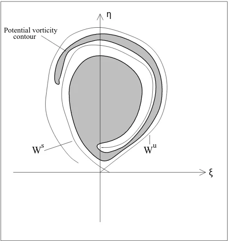
In addition to giving criteria on eddy growth, the Melnikov function enables us to qualitatively explain the presence of a tendril emanating from an eddy with one saddle point on its boundary. Tendrils often appear in the potential vortic-ity (or relevant scalar field) contours, as thin lobes which
η
ξ
W
Potential vorticity contour
s
W u
Fig. 7. A tendril of an eddy.
wrap around an essentially convex eddy structure (the exper-imental paper by Voropayev et al. (1999) shows some tendril structures). The presence of a tendril can be explained as a direct consequence of the fact that the diffusive contribu-tion to the Melnikov funccontribu-tion,Md, is constant. If the forcing
contribution is momentarily ignored, the Melnikov function would itself be constant, meaning that it is independent of the choice of the pointP (t )at which the measurement between Wu andWs is made. Now, since this constant is nonzero generically, this implies thatWs andWudo not intersect for any choice ofP (t ); i.e. near any point on the homoclinic. WhetherMis positive or negative, the consequence of con-stancy is a thin channel which opens up along the boundary of the eddy, as shown in Fig. 7. Fluid flows along this, in the basic direction of the flow on the manifolds, which causes the eddy to either grow or drain. In either case, however, trans-port occurs between the interior and exterior waters, which gradually homogenises the potential vorticity. Thus, interior waters would have potential vorticity values close to the val-ues along this channel. If viewing potential vorticity con-tours, this should be visible as a tendril, exactly as observed physically. Fig. 7 shows how an Eulerian potential vorticity contour might appear in the presence of fluid transport of this nature.
by observations (Voropayev et al., 1999).
We notice from equation (3) that the two processes which govern the potential vorticity transport are advection and dif-fusion (we are ignoring the forcing for the moment). In the purely diffusive process, the potential vorticity diffuses throughout the domain in the direction of−∇Q, indepen-dent of the flow. In addition, it advects; potential vorticity is carried by fluid particles following the flow. Note that what we have discussed so far is an advective effect, which causes fluid to flow into (the case of a growing eddy) or out of (draining eddy) the eddy along a tendril. Perhaps para-doxically, our advective process is created through a diffusive splitting of the eddy boundary; diffusion and advection com-bine to create these tendrils. If one imagines (3) as expressed in nondimensional coordinates, it is easy to see that the pure diffusive effect isO()(occurs on a time-scale of size 1/), whereas the advection velocity isO(1)(not small). How-ever, since the advective channel (the tendril) has sizeO(), the advective flux of potential vorticity has sizeO()as well: it also occurs on a time-scale of 1/. Thus, the advective and diffusive fluxes of potential vorticity have the same magni-tude. It is, therefore, unreasonable to ignore the advective effect in comparison with the purely diffusive effect when computing the potential vorticity balance for eddies.
A loose and intuitive understanding of tendrils could be that they result from the exterior portions of the eddy not being able to cope with the speed of rotation of the inte-rior, with diffusivity providing retardation. However, our interpretation enables a more geometric explanation for ten-drils. Diffusivity destroys the eddy boundary and creates a thin channel, along which an advective flux of potential vor-ticity occurs. This is not something which has been stated in the literature before; it is not an effect which can be ig-nored in comparison to pure diffusion of potential vorticity, with regard to eddy decay. This argument, in fact, works for any two-dimensional flow (not necessarily oceanographic) in which the relevant scalar quantity (not necessarily the poten-tial vorticity) is subject to an advection-diffusion equation with small diffusivity. The physical cause of such diffusion may be the effects of small scale turbulence, viscosity, etc. Therefore, our Melnikov approach provides a pleasing pos-sible explanation for eddy tendrils, as resulting from diffu-sivity breaking potential vorticity conservation.
Though the Melnikov approach provides information on how the manifolds perturb, it should be noted that the Mel-nikov function cannot describe how these manifolds behave after they wrap once around the homoclinic; the development is only valid for the first circuit of the manifolds around the homoclinic. Beyond this, the manifolds may wrap around and intersect in some complicated fashion, but any such ef-fects would be at distancesO(1)away from the unperturbed eddy boundary.
Should the eddy be defined by several saddle points on its boundary (rather than just one, as we have assumed in this paper), Melnikov functions would need to be calculated for each piece of the boundary which connects saddle points. However, the equations (9) and (10) cannot be applied in this
situation, and need modification for the fact that heteroclinic trajectories (rather than homoclinic) form the separatrices of interest. A constant value forMdis not obtained generically
for this heteroclinic case, and the quick argument for tendril formation outlined above cannot be made. Therefore, it is not clear whether this explanation generalises to more com-plicated eddy boundaries.
7 Forcing contribution
We briefly consider how the forcing contribution of the Mel-nikov function (10) can be analysed via geometric condi-tions on the eddy boundary. SinceMf(t )is dependent on t (unlike the diffusive contribution Md), it is more
diffi-cult to obtain simple criteria for eddy growth. Therefore, we will only inspect the geometry under several restric-tions, which are nevertheless of relevance in the Gulf Steam. Firstly, we shall specialise to standard models in which the flow is approximately steady in a eastward moving frame, as is commonly assumed (Pierrehumbert, 1991; del Castillo-Negrete and Morrison, 1993; Pratt et al., 1995). Then, we can set c2 = 0 (i.e., η = y). Secondly, we shall as-sume that the additional forcing is steady and meridional, i.e. f (x, y, t )=f (y)alone: a hypothesis which has been used in other oceanographic transport analyses in which the jet flow is mainly eastward (Poje and Haller, 1999). Thirdly, we shall suppose that the most southerly point of a warm eddy (or alternatively, the most northern point of a cold eddy) is its pinch-off point. This is a feasible assumption if addressing eddies in the process of pinching off from the Gulf Stream.
Under these conditions, the forcing contribution of the Mel-nikov function of (10) becomes
Mf =
Z ∞
−∞
[f (y(τ ))¯ −f (0)] dτ,
where(ξ ,¯ y)¯ is the parametrisation of the eddy boundary,η is identified precisely withy. We have replaced the moving frame forcingF withf, which additionally simplifies, since it has neitherx nort dependence. Under these simplifying assumptions, the forcing contribution is a constant and easy to analyse.
Consider the case, as usual, of a warm eddy. We have
¯
y(τ ) >0 for allτ, since the pinch-off point hasy-coordinate 0, and is assumed to be the most southerly point on the eddy boundary. Then, iff0(y) >0,Mf >0 and the contribution
shall be a growing one. On the other hand, if we take a cold eddy, we havey(τ ) <¯ 0 for allτ, and iff0(y) >0, we would obtainMf <0: again the correct sign towards eddy growth.
previous section, we note that even if our qualitative con-dition(s) should not be satisfied exactly, the eddy may still grow if those qualities contribute sufficiently. We addition-ally stress that, in reality, it is the combined effect of all the contributions (diffusive and forcing) which give the eddy its growth instructions. Since the geometry changes dynami-cally, it is possible that the eddy grows at some times, and shrink at others.
8 Conclusions
This paper has analysed the qualitative structure of an eddy (Eulerian definition) which contributes towards its growth, and hence, its stability in a specific sense. All eddies of length scales greater than that corresponding to turbulent eddy diffusivities can be addressed through this viewpoint, which, therefore, includes both mesoscale and submesoscale eddies. The effective dynamics are considered a perturbation of potential vorticity conserving flow; the perturbation result-ing directly from the inclusion of diffusion (and an additional small wind forcing) in the dynamical equation. Four qualita-tive observations were obtained in Sect. 5 which are indica-tive of eddy growth: (i) acute pinch-angle, (ii) small poten-tial vorticity gradient across the eddy boundary, (iii) large ra-dius of curvature of the eddy boundary, and (iv) the potential vorticity contours more tightly packed just within the eddy than outside. These conditions apply for both warm-core and cold-core eddies. If the wind forcing is meridional and steady, and the pinch-off point of the eddy is its most south-ernly (resp. most northsouth-ernly) point for a warm (resp. cold) eddy, then another such contributory factor towards growth is that the wind forcing increases in the northward direction. The actual behaviour of the eddy depends upon the combina-tion of all these factors.
Our eddy growth criteria are simple geometric conditions, which should be verifiable if potential vorticity data of a suit-able resolution is availsuit-able. The power of these conditions is that no knowledge of the velocity field is necessary. For the diffusive contributions, in fact, the criteria depend only on potential vorticity contours! The conditions are based, in re-ality, on the unperturbed potential vorticity contours, but for a ‘nearly’ potential vorticity conserving flow (such as believed to be true of oceanic jets and eddies); the perturbed contours could be expected to provide a sufficiently close approxima-tion to the unperturbed ones. In any case, ours is a completely new approach to eddy stability in the presence of small dif-fusion, characterised by simple qualitative statements on the geometry of the potential vorticity field.
Paldor (1999), in analysing linear stability of discontin-uous, radially symmetric, barotropic vortices, states in his abstract that if “the potential vorticity is continuous” at the boundary, “details of potential vorticity become important.” Though in a different context, it is instructive that in our analysis of continuous potential vorticity models, it is ex-actly such details of potential vorticity contours which arise as conditions for eddy stability.
An added bonus from our arguments is that they give a possible explanation for tendrils which are often observed emanating from eddy structures. Diffusivity provides the mechanism for the breaking of the eddy boundary into a thin channel along the eddy boundary, where potential vorticity is advected. The potential vorticity contours develop a ten-dril along this channel as a result of the advection. Since the advection velocities are not small, these tendrils should be easily visible if diffusivity is present in the system. This is a generic effect for eddies with exactly one saddle point on their boundaries, and is to be expected whenever the con-servation of a scalar field is broken through the inclusion of small diffusivity.
Acknowledgement. Conversations with Leonid Kuznetsov are grate-fully acknowledged. Both authors were supported in part by the NSF through grant DMS-97-04906, and the ONR through grant N-00014-92-J-1481.
References
Balasuriya, S., Vanishing viscosity in the barotropic β-plane, J. Math. Anal. Appl., 214, 128–150, 1997.
Balasuriya, S., Jones, C. K. R. T., and Sandstede, B., Viscous per-turbations of vorticity-conserving flows and separatrix splitting, Nonlinearity, 11, 47–77, 1998.
Biferale, L., Crisanti, A., Vergassola, M., and Vulpiani, A., Eddy diffusivities in scalar transport, Phys. Fluids, 7, 2725–2734, 1995.
Caflisch, R. and Sammartino, M., Zero viscosity limit for analytic solutions of the Navier-Stokes equation on a half-space. II. Con-struction of the Navier-Stokes solution, Commun. Math. Phys., 192, 463–491, 1998.
Brown, M. G. and Samelson, R. M., Particle motion in vorticity-conserving, two-dimensional incompressible flow, Phys. Fluids, 6, 2875–2876, 1994.
del Castillo-Negrete, D. and Morrison, P. J., Chaotic transport by Rossby waves in shear flow, Phys. Fluids A, 5, 948–965, 1993. Dewar, W. K. and Gailliard, C., The dynamics of barotropically
dominated rings, J. Phys. Oceanography, 24, 5–29, 1994. Dewar, W. K. and Killworth, P. D., On the stability of oceanic rings,
J. Phys. Oceanography, 25, 1467–1487, 1995.
Dewar, W. K., Killworth, P. D., and Blundell, J. R., Primitive-equation instability of wide oceanic rings. Part II: Numerical studies of ring stability, J. Phys. Oceanography, 29, 1744–1758, 1999.
Fannjiang, A. and Papanicolaou, G., Convection enhanced diffusion for periodic flows, SIAM J. Appl. Math., 54, 333–408, 1994. Fenichel, N., Persistence and smoothness of invariant manifolds of
flows, Indiana Univ. Math. J., 21, 193–226, 1971.
Flierl, G. R., On the instability of geostrophic vortices, J. Fluid Mech., 197, 349–388, 1988.
Guckenheimer, J. and Holmes, P., Nonlinear Oscillations, Dynam-ical Systems, and Bifurcation of Vector Fields, Springer, New York, 1983.
Haidvogel, D. B., Robinson, A. R., and Booth, C. G. H., Eddy in-duced dispersion and mixing, in Eddies in Marine Science, A. R. Robinson, (Ed.), Springer, Berlin, 1983.
oceanographic flows, Nonlinear Processes in Geophys., 4, 223– 235, 1997.
Helfrich, K. R. and Send, U., Finite-amplitude evolution of two-layer geostrophic vortices, J. Fluid Mech., 197, 331–348, 1988. Hirsch, M. W., Pugh, C. C., and Shub, M., Invariant Manifolds
(Lecture Notes in Mathematics 583), Springer, Berlin, 1977. Jones, S. W., Interaction of chaotic advection and diffusion, Chaos
Solitons Fractals, 4, 929–940, 1994.
Klapper, I., Shadowing and the role of small diffusivity in the chaotic advection of scalars, Phys. Fluids A, 4, 861–864, 1992. McWilliams, J. C., Gent, P. R., and Norton, N. J., The evolution of
balanced, low-mode vortices on theβ-plane, J. Phys. Oceanog-raphy, 16, 838–855, 1986.
Mezi´c, I., Brady, J. F., and Wiggins, S., Maximal effective diffusiv-ity for time-periodic incompressible flows, SIAM J. Appl. Math., 56, 40–56, 1996.
Miller, P., Jones, C. K. R. T., Rogerson, A. M., and Pratt, L. J., Quantifying transport in numerically generated velocity fields, Physica D, 110, 105–122, 1997.
Paldor, N., Linear instability of barotropic submesoscale coherent vortices observed in the ocean, J. Phys. Oceanography, 29, 1442– 1452, 1999.
Pierrehumbert, R. T., Chaotic mixing of tracer and vorticity by mod-ulated travelling waves, Geophys. Astrophys. Fluid Dyn., 58, 285–319, 1991.
Pedlosky, J., Geophysical Fluid Dynamics, Springer, New York,
1987.
Poje, A. C. and Haller, G., Geometry of cross-stream mixing in a double-gyre ocean model, J. Phys. Oceanography, 29, 1649– 1665, 1999.
Poje, A. C., Haller, G., and Mezi´c, I., The geometry and statistics of mixing in aperiodic flows, Phys. Fluids, 11, 2963–2968, 1999. Pratt, L. J., Lozier, M. S., and Beliakova, N., Parcel trajectories in
quasi-geostrophic jets: neutral modes, J. Phys. Oceanography, 25, 1451–1466, 1995.
Richardson, P. L., Gulf Stream rings, in Eddies in Marine Science, Robinson, A.R. (ed.), Springer, Berlin, 1983.
Robinson, A. R., Overview and summary of eddy science, in Eddies in Marine Science, Robinson, A.R. (ed.), Springer, Berlin, 1983. Rogerson, A. M., Miller, P. D., Pratt, L. J., and Jones, C. K. R. T., Lagrangian motion and fluid exchange in a barotropic meander-ing jet, J. Phys. Oceanography, 29, 2635–2655, 1999.
Rom-Kedar, V. and Poje, A. C., Universal properties of chaotic transport in the presence of diffusion, Phys. Fluids, 11, 2044– 2057, 1999.
Voropayev, S. I., McEachern, G. B., Boyer, D. L., and Fernando, H. J. S., Experiment on the self-propagating quasi-monopolar vor-tex, J. Phys. Oceanography, 29, 2741–2751, 1999.
Weiss, J. B., Hamiltonian maps and transport in structured fluids, Physica D, 76, 230–238, 1994.