https://doi.org/10.5194/soil-3-235-2017
© Author(s) 2017. This work is distributed under the Creative Commons Attribution 4.0 License.
SOIL
Planning spatial sampling of the soil from an uncertain
reconnaissance variogram
R. Murray Lark1, Elliott M. Hamilton1, Belinda Kaninga2,3, Kakoma K. Maseka4, Moola Mutondo4, Godfrey M. Sakala2,3, and Michael J. Watts1
1Centre for Environmental Geochemistry, British Geological Survey,
Keyworth, Nottinghamshire, NG12 5GG, UK
2Zambia Agriculture Research Institute, Mount Makulu, Central Research Station, Lusaka, Zambia 3University of Zambia, Great East Road Campus, Lusaka, Zambia
4Copperbelt University, Jambo Drive, Riverside, Kitwe, Zambia
Correspondence:R. Murray Lark ([email protected])
Received: 27 July 2017 – Discussion started: 21 August 2017
Revised: 27 October 2017 – Accepted: 7 November 2017 – Published: 13 December 2017
Abstract. An estimated variogram of a soil property can be used to support a rational choice of sampling intensity for geostatistical mapping. However, it is known that estimated variograms are subject to uncertainty. In this paper we address two practical questions. First, how can we make a robust decision on sampling intensity, given the uncertainty in the variogram? Second, what are the costs incurred in terms of oversampling because of uncertainty in the variogram model used to plan sampling? To achieve this we show how samples of the posterior distribution of variogram parameters, from a computational Bayesian analysis, can be used to characterize the effects of variogram parameter uncertainty on sampling decisions. We show how one can select a sample intensity so that a target value of the kriging variance is not exceeded with some specified probability. This will lead to oversampling, relative to the sampling intensity that would be specified if there were no uncertainty in the variogram parameters. One can estimate the magnitude of this oversampling by treating the tolerable grid spacing for the final sample as a random variable, given the target kriging variance and the posterior sample values. We illustrate these concepts with some data on total uranium content in a relatively sparse sample of soil from agricultural land near mine tailings in the Copperbelt Province of Zambia.
1 Introduction
When one plans a spatial survey of a soil property by geo-statistical mapping, a key choice is the intensity of sampling effort (samples per unit area or, equivalently, spacing of a regular sampling grid). This decision determines the overall cost of sampling but also the precision of the predictions and therefore the uncertainty in the resulting information. It has long been recognized that, when the variogram of the target variable is known, either by reconnaissance sampling or from data in a homologous environment, it is possible to compute the prediction error variances (kriging variance) for sampling grids of different intensity and so to find the amount of sam-ple effort that is required to meet a target level of precision of the spatial predictions (McBratney et al., 1981). This
ap-proach has been used in practice (e.g. Di et al., 1989; Ruffo et al., 2005). However, it is often the case that the num-ber of observations available from reconnaissance survey is rather limited, which means that the estimated variogram has considerable uncertainty. This uncertainty in the variogram propagates through the calculation of kriging variance, so the kriging variance achieved by a particular grid spacing has an attendant uncertainty.
of data for sample planning purposes, except in the case of large surveys on a national scale. An alternative approach was proposed by Marchant and Lark (2006). This is an adap-tive sampling strategy in which data are collected in dis-crete phases. The distribution of sample points for the initial sampling phase is optimized to minimize uncertainty in var-iogram parameters, given a wide prior distribution for these. In subsequent phases this initial sample is supplemented to improve the precision of the estimates of variogram param-eters until the uncertainty in the final sample grid spacing required to complete the survey is reduced to an acceptable size. An advantage of this approach is that the total sam-ple effort is controlled by the evaluation of the quality of information available at the end of each phase, and so the information provided by an initial phase with rather fewer than 100 samples can be exploited. We make no arbitrary as-sumptions about the requisite sample size. A disadvantage, however, is that it is not always feasible to divide a sampling campaign into several phases, particularly if the region to be surveyed is remote, the samples take a significant time to pro-cess and analyse, or the target variable is subject to change over time. Marchant and Lark (2006) suggested that there may, nonetheless, be benefits in simple two-phase optimized designs in which information obtained in the first phase of sampling is used in a numerical optimization procedure to find the distribution of sample points, given those already sampled in phase 1, which minimizes some measure of pre-diction uncertainty.
These tools for optimization are powerful, but they are computationally costly. Furthermore, they address directly the question of how to deploy some specified number of sample points and are cumbersome if the initial question is what survey intensity is required because this requires a la-borious optimization of the distribution of different numbers of sample points. In this paper we consider a simpler ap-proach where the basic procedure of McBratney et al. (1981) is adapted to account for uncertainty in the estimated vari-ogram parameters as quantified in a Bayesian analysis. Such an approach might be useful for making initial decisions on sample effort even if the final distribution of points is opti-mized using methods such as those of Marchant and Lark (2007).
In this paper we consider a case study from the Copper-belt Province in Zambia. A reconnaissance survey was un-dertaken on farmland in close proximity to a mine tailings dam. This survey was based on a nested sampling design (Lark et al., 2017), of which we report on 64 samples which were collected at a site of interest, the land farmed by the in-habitants of Mugala village near Kitwe. This sample size is rather fewer than the minimum of 100 suggested by Webster and Oliver (1992).
One variable measured in this survey was the total content of uranium (U) in the soil, and it is that variable which we examine here. Uranium is of interest because the process-ing of copper ore can produce technically enhanced
natu-rally occurring radioactive material (TENORM) in the tail-ings (residual waste) through the concentration of radionu-clides, including uranium. Uranium is known to be a signifi-cant constituent of TENORM in wastes produced from cop-per mines in the Katanga Basin, which includes the Zambian Copperbelt (Katebe et al., 2008).
In this paper we present a Bayesian geostatistical analysis of the data and show how this allows us to quantify the effects of variogram uncertainty on the inferred precision of predic-tions from sample grids of different spacing and to support a robust choice of sample intensity.
2 Materials and methods
2.1 Field work and data collection
The study area was approximately 18 ha of farmland used by the inhabitants of Mugala village near Kitwe, located in the Copperbelt Province in the north of Zambia, (12◦47016.100S 28◦6013.200E). According to the Exploratory Soil Map of Zambia (1 : 1 000 000), (Ministry of Agriculture, 1991), the soils at and around Kitwe are mapped as plateau soils (leg-end unit Pu7) which comprises Chromi-haplic Acrisols with Gleyi-haplic Acrisols and partly skeletal phase Dystric Lep-tosols according to the then-current FAO soil classification (FAO-Unesco, 1974).
A full account of the sampling undertaken in this study is provided by Lark et al. (2017). The sampling was undertaken on transects with sample main stations at intervals of 100 to 200 m. At each main station a soil sample was collected. A second point was collected 100 m from the main station in a direction approximately normal to the direction of the transect. A third sample point was selected 10 m from the second in a random direction and a fourth point 1 m from the third, again in a random direction. The soil samples at each sample point were composites, formed by bulking five cores taken with a Dutch auger (15 cm depth of soil from the surface and 5 cm in diameter). These cores were taken from the corners and centre of a square of approximately 30 cm length. The samples were placed in paper sample bags, and a few days after collection each sample was reduced in size by coning and quartering. A total of 64 samples were collected this way at Mugala village.
2.2 Data analysis
2.2.1 The linear mixed model and its parameters Summary statistics were computed for the data, and their spa-tial distribution was examined. The assumption of a station-ary mean seemed plausible from the post plot of the data (Fig. 1b) and the transitive behaviour of the empirical var-iogram which does not increase at lags longer than about 300 m (Fig. 2a); so a linear mixed model was proposed for the n data, in which they are treated as a realization of a second-order stationary random variable,Z. The model takes the following form:
z=µ+η+ε, (1)
whereµis a vector, lengthn, with all values equal to a con-stant mean, andη andεare mutually independent random effects. The componentηis distributed as
η∼N0n, ξ σ2R
, (2)
andεis distributed as
ε∼N0n,(1−ξ)σ2In
, (3)
where0n is a vector lengthnwith all elements equal to 0; In is ann×nidentity matrix;Ris ann×ncorrelation ma-trix; σ is the overall variance of Z, withξ σ2 the variance of the spatially correlated component, η, and (1−ξ)σ2 the variance of the independently and identically distributed el-ement, ε. The spatial correlation is modelled under the as-sumption of second-order stationarity (Webster and Oliver, 2007) such that elementRi, jof the correlation matrix can be modelled as a function of the lag interval between theith andjth observations at locationssiandsjrespectively. With a small data set, we assume that the correlation depends only on the length of the lag vectorh= |si−sj|. In this study we used the Matérn correlation function (Matérn, 1986):
ρ(h)=n2κ−10(κ)o −1h
φ κ
Kκ
h
φ
, (4)
where 0(·) is the gamma function and Kκ is a modified Bessel function of the second kind of order κ. The two pa-rameters are κ, a smoothness parameter, andφ, a distance parameter. These have to be estimated in addition to the vari-anceσ2and the parameterξ, which represents the proportion of the variance which is spatially dependent.
Under the linear model with a constant mean the variance parameters κ, φ,σ2 andξ can be estimated by maximum likelihood (Lark, 2000; Zimmerman and Stein, 2010; Dig-gle and Ribeiro, 2007). It is known that the first of these pa-rameters can be difficult to estimate, and Diggle and Ribeiro (2007) suggest that, rather than estimating it along with the other parameters, the marginal likelihood is obtained for a set of discrete values of the parameter (i.e. the likelihood maxi-mized with respect to all the other parameters whenκis fixed
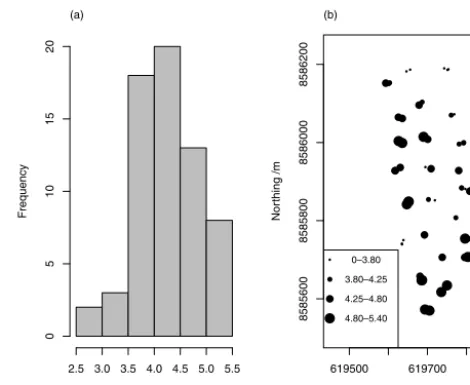
Figure 1.(a)Histogram of uranium concentrations in soil sam-ples and(b) post plot showing the spatial distribution of sample points with symbols indicating concentration intervals delimited by the range and empirical quartiles. The eastings and northings are according to the Universal Transverse Mercator projection zone 35.
at a specified value). Examination of the profile negative log-likelihood function for theκ parameter showed that it was potentially troublesome to estimate. Although the negative log likelihood was smaller with κ=2 than with larger or smaller values, the slope of the marginal likelihood asκwas increased above 1.5 was very small. For this reason we fol-lowed the guidance of Diggle and Ribeiro (2007) and fixed κ at the value for which the profile negative log likelihood was smallest: 2.0. All subsequent analyses are conditional on this choice. Smaller values ofκare not implausible, given the shape of the likelihood profile. Selecting 2.0 rather than a smaller value is likely to lead to larger estimates of the un-correlated “nugget” variance, which will tend to imply larger kriging variances and so is conservative.
Estimates of the other variance parameters were obtained by maximum likelihood. It is possible to quantify uncertainty in these estimates by treating the inverse of the Fisher in-formation matrix as an estimate of the covariance matrix of estimation errors (e.g. Dobson, 1990), but this requires as-sumptions of linearity which are not plausible for all of the parameters, notably the distance parameter (Marchant and Lark, 2004). An alternative approach is to use a Bayesian formulation of the linear mixed model under which the vari-ance parameters are treated as random variables with a prior distribution, updated to give a posterior distribution by refer-ence to available data. This has been done in previous studies with the linear mixed model applied to soil data (e.g. Orton et al., 2009; Minasny et al., 2011).
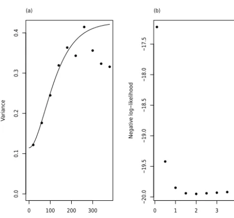
Figure 2. (a)Method-of-moments estimates of the variogram of soil uranium content with the maximum likelihood estimate of the variogram superimposed.(b)Profile values of the negative log like-lihood for different values of theκparameter.
variance parameters is drawn. This sample can then be used for further inference about the parameters. Both Orton et al. (2009) and Minasny et al. (2011) used this approach, and we follow the latter in using the “dream” algorithm of Vrugt et al. (2009), as implemented for the R platform (R develop-ment core team, 2014) by Guillaume and Andrews (2012) for the analysis. For details of this method the reader is re-ferred to Vrugt (2016). In summary, the “dream” algorithm runs multiple MCMC chains in parallel and automatically tunes the “proposal” distribution, which is used to perturb the values in each chain and explore the parameter space so that the resulting sequence of samples has desirable statis-tical properties. In “dream”, and other multichain methods, the perturbation of the chains in each generation is obtained as a combination of a random variate and the difference be-tween the parameters values for randomly selected pairs of chains. In “dream”, computational efficiency is achieved by updating only random subsets of the parameters in each gen-eration and by special treatment to identify and manage out-lier chains. We used nine chains in our analysis for three pa-rameters, with four chain pairs used to generate the jump at each sample. Other “dream” parameters were set at default values which we have found to be robust over a range of set-tings. The first 10% of values in each chain was discarded to avoid the effects of the burn-in period, which is influenced by initial arbitrary settings. Every tenth output of the chain was selected for the final sample to reduce the effects of autocorrelation between samples. The prior distribution for the variogram parameters was uniform over the admissible range [0,1]for ξ. For the other parameters the priors were
uniform for positive values up to a maximum (10 and 1000 respectively forσ2andφ). It is important to recall that in a Bayesian analysis all inference is conditional on the priors. In the absence of strong evidence to constrain uniform prior distributions, it is good practice to choose sufficiently wide bounds such that the posterior probability density is negligi-ble near extremes (Diggle and Ribeiro, 2007). On this basis the selected bounds for the prior distributions ofσ2 andφ were judged to be acceptable.
2.2.2 Kriging variance as a random variable
In the analysis undertaken here the smoothness parameterκ was fixed at the value selected from the profile likelihood, but the other parameters,φ,σ2andξ, comprise a set which is treated as a random variate:
2=
n
8, 62, 4 oT
, (5)
of which we havemMCMC samples:
θi=
n
φi, σi2, ξi
oT
, i=1, . . ., m.
For someθ, and conditional on a specified interval for a square sample grid,λ, one can compute the kriging variance at the centre of a grid cell. In this paper we consider the ordi-nary kriging variance. We may write this kriging variance as a function ofθ:
vk,λ=f(θ|λ). (6)
In our Bayesian formulation of the problem, the variogram parameters are treated as random variables, and so we may treat the kriging variance, conditional onλ, as a random vari-able:
Vk,λ=f(2|λ). (7)
We may obtain a sample from this random variable by apply-ing the expression in Eq. (6) to each of themMCMC samples from2:
vk,λ,i=f(θi|λ,), i=1, . . ., m. (8)
From this sample we may obtain an estimate of the mean kriging variance,vk,λwith the specified grid spacing. We can also compute an empirical estimate of the distribution func-tion forvk,λ:
b
F(v|λ,) = #v≤k,λv/m, (9)
wherev≤k,λv is the sub-vector comprising all elements ofvk,λ which are≤v.
achieved by some grid spacing,λ, is uncertain. One way to deal with this is to ensure that the probability that the tar-get kriging variance is not exceeded for a chosen spacing is sufficiently large. This is analogous to power analysis for hy-pothesis testing. If we specify a probability of, for example, 0.8, then we could select a grid spacing,λ˘such that
b Fvt| ˘λ
=0.8. (10)
We undertook these calculations using the sample of var-iogram parameters obtained from the MCMC chains as de-scribed in the previous section. The kriging variance for each sample was computed for the cell centre of square sample grids considering spacings up to 300 m.
The target kriging variance,vt, might be selected on vari-ous grounds (de Gruijter et al., 2006; Black et al., 2008; Lark and Knights, 2015). For illustrative purposes we chose to se-lect a target kriging variance such that the kriging standard error was 10 % of the overall mean concentration. This gives a target kriging variance ofvt=0.18 in this case.
We computed, for each of a set of grid spacings up to 300 m, the estimate of Fb(vt|λ) and identified the spacing at which this value was 0.8.
2.2.3 Tolerable grid spacing as a random variable The previous section shows how one may select a grid spac-ing such that the probability that the krigspac-ing variance at the centre of a grid cell is less than or equal to a target variance is sufficiently large. We may then wish to quantify the impli-cations of the uncertainty in terms of the extent to which we are likely to have oversampled to account for it. To do this we introduce the notion of the tolerable grid spacing as a random variable given uncertainty in the variogram parameters.
For some sample from the variogram parameters,θ, it may be possible to findλv, the spacing of a square grid such that the kriging variance at the centre of a grid cell is v. This is done numerically, by interpolation between evaluations of the kriging variance for a series of grid spacings and the par-ticular parameter set using Eq. (6). The valueλvis not nec-essarily defined for some parameter set,θ. There are two cir-cumstances in which it is not. The first is when
v > σ2+ψλ,∀λ, (11)
where ψλ denotes the Lagrange parameter of the ordinary kriging estimate at the centre of a grid cell of spacingλ. In this circumstance the target kriging variance is so large that it is matched by kriging from the coarsest grid. The second circumstance in whichλvis not defined is when the spatially uncorrelated variance is larger thanv:
v < ξ σ2. (12)
In this latter case the kriging variancev cannot be achieved at the centre of the grid cell however fine the spacing. When
ξ σ2< v < σ2+ψλ∀λ,
then a unique value ofλvis defined for theθandvunder con-sideration, assuming ordinary point kriging or block kriging for a block which is small compared with the grid of obser-vations from which the prediction is made. Whenvtakes a value in the range for whichλv is defined, we may express the relationship by a function:
λv=g(v,θ). (13)
We callλvthe tolerable grid spacing because it is the coars-est spacing compatible with the kriging variancev. In the Bayesian approach, whereθ is drawn from a random vari-able2, we can treat the tolerable grid spacing as a random variable3v:
3v=g(v,2). (14)
Consider a situation in which an oracle provides variogram parameters without uncertainty and we can therefore com-pute the tolerable grid spacing for target variance vt with-out uncertainty. The sample density isλ−vt2samples per unit area. If, in the same circumstances, we did not have access to the oracle but selected a grid spacing,λ˘, to achieve Eq. (10), then the oversampling, attributable to our strategy to man-age uncertainty would beλ˘−2−λ−v2
t samples per unit area.
This could be directly translated to a cost given analytical costs and logistical costs (e.g. Lark and Knights, 2015). In practice we may use ourmMCMC samples of the variogram parameters,θi, to compute a set of tolerable grid spacings, where this is defined as
λvt,λ,i=g(vt,θi); if ξiσ
2
i < v < σi2+ψλ∀λ; (15) i=1, . . ., m.
Table 1.Summary statistics on soil uranium content.
n 64
Mean (mg kg−1) 4.29 Median (mg kg−1) 4.25 Standard deviation (mg kg−1) 0.60 Skewness −0.13
Table 2.Maximum likelihood estimate of spatial covariance param-eters for soil uranium.
φ(m) 55.50
κ∗ 2
σ2 0.43
ξ 0.73
∗Obtained by profile likelihood.
be attractive when a survey is planned over a large region, and additional sampling effort is small relative to the total sample effort expected.
We followed these procedures, using Eq. (15) to compute a sample of tolerable grid spacings for the target kriging vari-ance of 0.18. We noted the proportion of samples for which this tolerable grid spacing was defined. We computed the cor-responding values of the sample density.
We then repeated these calculations assuming that (i) the target kriging variance is 0.18 but that we are prepared to accept a smaller probability that it is not exceeded (0.75 or 0.70) and (ii) that we can accept a larger target kriging vari-ance of 0.25 but require a probability of 0.8 that it is not exceeded.
3 Results
Table 1 shows summary statistics for the data on uranium, and their histogram is shown in Fig. 1a. The data are rea-sonably symmetrically distributed, and there is no evidence from these data that a transformation is required. The empir-ical variogram (solid symbols in Fig. 2a) shows no evidence of a spatial trend. The profile negative log likelihoods for dif-ferent values of theκparameter are shown in Fig. 2b. On the basis of these resultsκ was fixed at 2.0. The maximum like-lihood estimates of the parameters are presented in Table 2, and the solid line in Fig. 2a shows the corresponding vari-ogram.
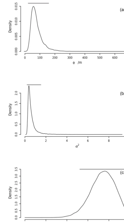
Figure 3 shows the empirical posterior distributions of the three variogram parameters (conditional on fixingκ=2) corresponding to 15 282 samples after removing the first 10 % for burn-in and then extracting every tenth. Note that the empirical density is small near the upper prior limit for φ (1000 m) and for σ2 (10). The horizontal bars show the 95 % credible intervals for each parameter. Because the dis-tributions are not symmetrical, the credible intervals were the
Figure 3.Empirical probability density functions for variogram pa-rameters:φ(a),σ2 (b)andξ (c). These were obtained from the MCMC samples. Horizontal bars show the 95 % credible interval for each parameter.
highest density intervals (i.e. for a unimodal distribution the narrowest interval over which the integral of the probabil-ity densprobabil-ity is 0.95). This was computed using the “hdi” pro-cedure from the “HDInterval” package for the R platform (Meredith and Kruschke, 2016).
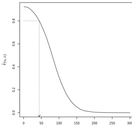
Figure 4.Estimates ofFb(vt|λ,) (Eq. 9) for different grid spacings
withvtset to 0.18. The dotted line shows the grid spacing (44.2 m)
at whichFb(vt|λ,)=0.8.
in Fig. 5, and the target kriging variance is equivalent to a grid spacing of 85 m (1.38 samples ha−1).
Treating the grid spacing which achieves the target krig-ing variance of 0.18 as a random variable,3vt(tolerable grid
spacing), we found that this was defined for 99.22 % of the MCMC samples. Figure 6a shows the empirical probability density function (PDF) of the grid spacings,λvt. This
distri-bution is mildly positively skewed with some values in an upper tail, but the mean (86.4 m) and median (84.4 m) are very close. The distribution of corresponding sample densi-ties (rescaled to samples per ha) is strongly skewed and is shown on a log scale in Fig. 5b. The median tolerable sample spacing is 1.4 samples ha−1, the mean is strongly influenced by the upper tail, and its value (5.32 samples ha−1) is the 87th empirical percentile of the observations. For this reason we summarize the distribution of tolerable sample densities by its median.
We can now summarize the practical implications of this analysis for further sampling of the soil to map uranium in this environment or comparable ones. The variogram is un-certain, which is not surprising given the relatively small sample size. Because of this, for any specified sample grid spacing, we cannot be sure about the expected prediction er-ror variance at the centre of a grid cell because this depends on variogram parameters about which we are uncertain. If a decision on sample density were based on the empirical variogram parameters alone, with no attention to their un-certainty, then these results show that the sample effort re-quired to ensure that prediction error variances are below some threshold may be markedly underestimated.
On the basis of our Bayesian analysis we can characterize the uncertainty in the variogram parameters, and so we can
Figure 5.Value of kriging variance at the centre of a square grid cell as a function of grid spacing,λ. The solid line is the expected value of kriging variance over the distribution of parameters, and the dashed line are the values given the maximum likelihood estimates of those parameters.
Figure 6.Empirical probability density function for grid spacing that achieves the target kriging variance (0.18) and corresponding PDF for the logarithm of the sample density which achieves the same.
The achievement of this level of confidence in the quality of our final spatial predictions comes with a cost; we have to do more sampling than we would if the variogram parame-ters were known with greater certainty. Our analysis shows that the median-unbiased tolerable grid spacing for the tar-get variance is 1.4 samples ha−1 (close to what we would have obtained if we used the maximum likelihood estimate of the variogram parameters to find the grid spacing). This means that the median-unbiased oversampling due to the un-certainty is 3.72 samples ha−1. This could be a substantial cost for a survey of a large region.
If this cost is unacceptable, then there are three approaches we could take. The first is to allow greater uncertainty that our final predictions are of the target precision. We consid-ered the effect of basing the sampling decision on a smaller probability that the target kriging variance is not exceeded, with the target kriging variance held at 0.18. If we specify a probability of 0.75 rather than 0.8, then the grid spacing increases to 53 m (sample density of 3.54 per ha) and the median-unbiased oversampling due to uncertainty is reduced to 2.1 per ha. Reducing the probability further to 0.7, the grid spacing is 56 m, and the sample density is 3.13 per ha, with a median-unbiased over sampling of 1.7 per ha.
A second approach is to accept a larger target kriging vari-ance. We considered a value of 0.25. The probability that this is not exceeded is 0.8 with a grid spacing of 110 m (0.82 sam-ples ha−1), and the median-unbiased oversampling in this case is 0.38 samples ha−1(the tolerable grid spacing was de-fined for 97 % of cases because of the increased probability that the kriging variance would be bounded at a smaller value than the target).
Both these approaches require that we tolerate greater un-certainty, either in the final predictions (accepting a larger kriging variance) or our level of confidence that the specified kriging variance is achieved. If neither of these is acceptable, then we must collect additional data to reduce the uncertainty in the variogram model before planning the final survey.
4 Conclusions
In this paper we have introduced two new concepts for use in the planning of a geostatistical survey. In the first we consider the kriging variance achieved with a particular grid spacing as a random variable, given a set of MCMC samples of the variogram parameters. This allows us to select a grid spacing such that the probability that the target kriging variance is not exceeded is met with a specified probability. The second concept is to treat the tolerable grid spacing as a random vari-able. This allows us to quantify the effects of variogram un-certainty in terms of expected oversampling. These provide a framework for decision-making about geostatistical sam-pling based on an uncertain variogram. We have shown that, for some plausible values of the target kriging variance, and required probability that the kriging variance is not exceeded,
it may be necessary to accept that considerable oversampling is necessary. This can be reduced by changing either condi-tion. The scientist planning sampling, or stakeholders such as regulator or policy makers, can explore the effect of relaxing either the target kriging variance or the probability that it is not exceeded.
An alternative, if the expected oversampling is large, is to put some additional sampling effort into improving the qual-ity of the variogram estimate on which the final survey is to be based. Within the Bayesian framework, we cannot com-pute an expected effect on the parameter uncertainty of in-cluding some specified number of additional sample points. However, we could optimize the distribution of the additional points using the procedures of Marchant and Lark (2006), and if the amount of additional sampling is limited to, for example, 10 % of the median-unbiased estimate of oversam-pling incurred with the uncertainty in the current variogram, that will ensure that additional sampling to improve the vari-ogram is not excessive.
There is scope for further work on the methods presented in this paper. First, we note that the study is based on or-dinary kriging, in which the mean is assumed to be station-ary. The method could be extended to more general cases of the empirical best linear unbiased predictor (e.g. univer-sal kriging). In this case, however, the prediction error vari-ance has a component due to uncertainty in the parameters which describe the non-stationary mean (e.g. coefficients of a trend surface). The computed prediction error variance for different sample strategies will therefore be conditional on assumptions about the model for the mean (e.g. that it is a second-order polynomial in the rectilinear coordinates). The approach could be extended to encompass other sources of uncertainty in the variogram model (e.g. measurement or lo-cation error) or the use of a variogram estimated from geo-physical data which can be regarded only as a proxy for the target variable, provided that these uncertainties can be in-corporated into a Bayesian formulation.
Second, in this study we considered a uniform sample grid, which is appropriate for sampling a relatively large and uni-form region. It would be straightforward to do the same com-putations on sample designs obtained for non-uniform re-gions by spatial coverage methods such as those presented in the “spcova” package for the R platform (Walvoort et al., 2010).
on detailed sampling for mapping or whether additional ex-ploratory sampling is needed before a final survey design is fixed. In summary, the practical guidelines for sample plan-ning are as follows.
1. Identify a target kriging variance which represents an acceptable precision for the final spatial predictions of the soil property of interest.
2. Decide on a level of confidence, expressed in terms of a probability that the target precision is achieved, which is required for sample planning.
3. By a Bayesian analysis of available data, obtain samples from the posterior distributions of variogram properties, and from these identify the sample density required to achieve the target precision determined at step (1) with the probability determined at step (2).
4. Find the distribution of tolerable grid spacings, given the sample of variogram parameters, and from this com-pute the oversampling required to achieve the target pre-cision with acceptable probability.
5. If this level of oversampling is unacceptable, then either
i. review the decisions made at steps (1) and (2), in-creasing the acceptable kriging variance or reduc-ing the acceptable probability of achievreduc-ing this or both.
ii. plan additional sampling to improve the estimate of the variogram. The procedures presented by Marchant and Lark (2006) may be used to plan this additional sampling, but we cannot compute the re-quired additional sampling in the Bayesian frame-work. The amount of oversampling expected with current levels of uncertainty might provide a basis for deciding how much additional sampling to un-dertake at the reconnaissance stage.
Data availability. The original data are available as a Supple-ment to the online version of this paper, “Mugala_U.txt”. This is an ASCII file, each row corresponding to a sample site. The first two columns are eastings and northings (units of metres; Universal Transverse Mercator projection zone 35. The third column is the total U content in mg kg−1.
The Supplement related to this article is available online at https://doi.org/10.5194/soil-3-235-2017-supplement.
Competing interests. The authors declare that they have no con-flict of interest.
Acknowledgements. This paper is published with permission of the Executive Director of the British Geological Survey (Natural Environment Research Council). Field and laboratory work for this project was funded by The Centre for Environmental Geochemistry and BGS Global. Author contributions were supported by the UK Department for International Development (DFID) through a Royal Society and DFID Africa Capacity Building Initiative (ACBI) Programme Grant, Award AQ140000. We acknowledge the assistance of staff from ZARI and students at Copperbelt University for help with field sampling. We are grateful to the people of Mugala village for permission to sample on their fields. Edited by: Paul Hallett
Reviewed by: David Rossiter and one anonymous referee
References
Black, H., Bellamy, P., Creamer, R., Elston, D., Emmett, B., Frog-brook, Z., Hudson, G., Jordan, C., Lark, M. Lilly, A., Marchant, B., Plum, S., Potts, J., Reynolds, B., Thompson, P., and Booth, P.: Design and operation of a UK soil monitoring network, Envi-ronment Agency, Bristol, Science Report – SC060073, 2008. de Gruijter, J. J., Brus, D. J., Biekens, M. F. P., and Knotters, M.:
Sampling for Natural Resource Monitoring, Springer, Berlin, 2006.
Di, H. J., Trangmar, B. B., and Kemp, R. A.: Use of geostatistics in designing sampling strategies for soil survey, Soil Sci. Soci. Am. J., 53, 1163–1167, 1989.
Diggle, P. J. and Ribeiro, P. J.: Model-Based Geostatistics, Springer, New York, 2007.
Dobson, A. J.: An Introduction to Generalized Linear Models, Chapman & Hall, London, 1990.
FAO-Unesco: Soil Map of the World, 1 : 5 000 000, Volume 1, Leg-end, Unesco, Paris, 1974.
Guillaume, J. and Andrews, F.: dream: DiffeRential Evolution Adaptive Metropolis, R package version 0.4-2., available at: http: //dream.r-forge.r-project.org/ (last access: 8 December 2017), 2012.
Katebe, R., Michalik, B., Phiri, Z., and Nkhuwa, D. C. W.: Status of naturally occurring radionuclides in copper mine wastewater in Zambia, in: Proceedings of the Fifth International Symposium on Naturally Occurring Radioactive Material, International Atomic Energy Agency, Vienna, 409–417, 2008.
Lark, R. M.: Estimating variograms of soil properties by the method-of-moments and maximum likelihood; a comparison, Eur. J. Soil Sci., 51, 717–728, 2000.
Lark, R. M. and Knights, K. V.: The implicit loss function for errors in soil information, Geoderma, 251–252, 24–32, 2015.
Lark, R. M., Hamilton, E. M., Kaninga, B., Maseka, K. K., Mu-tondo, M., Sakala, G. M., and Watts, M. J.: Nested sampling and spatial analysis for reconnaissance investigations of soil: an ex-ample from agricultural land near mine tailings in Zambia, Eur. J. Soil Sci., 68, 605–620, 2017.
Marchant, B. P. and Lark, R. M.: Estimating variogram uncertainty, Math. Geol., 36, 867–898, 2004.
Marchant, B. P. and Lark, R. M.: Optimized sample schemes for geostatistical surveys, Math. Geol., 39, 113–134, 2007. Matérn, B.: Spatial Variation, Lecture Notes in Statistics, No. 36,
Springer, New York, 1986.
McBratney, A. B., Webster, R., and Burgess, T. M.: The design of optimal sampling schemes for local estimation and mapping of regionalised variables. I. Theory and Method, Comput. Geosci., 7, 331–334, 1981.
Meredith, M. and Kruschke, J.: HDInterval: Highest (Posterior) Density Intervals, R package version 0.1.3., available at: https:// cran.r-project.org/web/packages/HDInterval/index.html (last ac-cess: 8 December 2017), 2016.
Minasny, B., Vrugt, J. A., and McBratney, A. B.: Confronting uncertainty in model-based geostatistics using Markov Chain Monte Carlo simulation, Geoderma, 163, 150–162, 2011. Ministry of Agriculture: Exploratory Soil Map of Zambia, Scale
1 : 1.000.000, Ministry of Agriculture, Lusaka, 1991.
Orton, T. G., Rawlins, B. G., and Lark, R. M.: Using measurements close to a detection limit in a geostatistical case study to pre-dict selenium concentration in topsoil, Geoderma, 152, 269–282, 2009.
R Development Core Team: R: A language and environment for statistical computing, R Foundation for Statistical Computing, Vienna, Austria, available at: http://www.R-project.org/ (last ac-cess: 8 December 2017), 2014.
Ruffo, M. L., Bollero, G. A., Hoeft, R. G., and Bullock, D. G.: Spa-tial variability of the Illinois soil nitrogen test: implications for soil sampling, Agron. J., 97, 1485–1492, 2005.
Vrugt, J. A.: Markov chain Monte Carlo simulation using the DREAM software package: theory, concepts and MATLAB im-plementation, Environ. Model. Softw., 75, 273–316, 2016. Vrugt, J. A., Ter Braak, C. J. F., Diks, C. G. H., Robinson, B. A.,
Hy-man, J. M., and Higdon, D.: Accelerating Markov chain Monte Carlo simulation by differential evolution with self-adaptive ran-domized subspace sampling, Int. J. Nonlin. Sci. Num., 10, 273– 290, 2009.
Walvoort, D. J. J., Brus, D. J., and de Gruijter, J. J.: An R package for spatial-coverage sampling and random sampling from com-pact geographical strata by k-means, Comput. Geosci., 36, 1261– 1267, 2010.
Webster, R. and Oliver, M. A.: Sample adequately to estimate vari-ograms of soil properties, J. Soil Sci., 43, 177–192, 1992. Zimmerman, D. L. and Stein, M.: Classical geostatistical methods,