www.the-cryosphere.net/11/65/2017/ doi:10.5194/tc-11-65-2017
© Author(s) 2017. CC Attribution 3.0 License.
Fram Strait sea ice export variability and September Arctic
sea ice extent over the last 80 years
Lars H. Smedsrud1,2,3, Mari H. Halvorsen1, Julienne C. Stroeve4,5, Rong Zhang6, and Kjell Kloster7
1Geophysical Institute, University of Bergen, Bergen, Norway 2Bjerknes Centre for Climate Research, Bergen, Norway 3University Centre in Svalbard, Longyearbyen, Svalbard
4National Snow and Ice Data Centre, University of Colorado, Boulder, USA
5Centre for Polar Observation and Modelling, University College London, London, UK 6Geophysical Fluid Dynamics Laboratory, National Oceanic and Atmospheric Administration,
Princeton, New Jersey, USA
7Nansen Environmental and Remote Sensing Center, Bergen, Norway
Correspondence to:Lars H. Smedsrud (lars.smedsrud@uib.no)
Received: 1 April 2016 – Published in The Cryosphere Discuss.: 2 May 2016
Revised: 16 December 2016 – Accepted: 19 December 2016 – Published: 13 January 2017
Abstract.A new long-term data record of Fram Strait sea ice area export from 1935 to 2014 is developed using a combina-tion of satellite radar images and stacombina-tion observacombina-tions of sur-face pressure across Fram Strait. This data record shows that the long-term annual mean export is about 880 000 km2, rep-resenting 10 % of the sea-ice-covered area inside the basin. The time series has large interannual and multi-decadal vari-ability but no long-term trend. However, during the last decades, the amount of ice exported has increased, with sev-eral years having annual ice exports that exceeded 1 mil-lion km2. This increase is a result of faster southward ice drift speeds due to stronger southward geostrophic winds, largely explained by increasing surface pressure over Green-land. Evaluating the trend onwards from 1979 reveals an in-crease in annual ice export of about+6 % per decade, with spring and summer showing larger changes in ice export (+11 % per decade) compared to autumn and winter (+2.6 % per decade). Increased ice export during winter will gener-ally result in new ice growth and contributes to thinning in-side the Arctic Basin. Increased ice export during summer or spring will, in contrast, contribute directly to open water further north and a reduced summer sea ice extent through the ice–albedo feedback. Relatively low spring and summer export from 1950 to 1970 is thus consistent with a higher mid-September sea ice extent for these years. Our results are not sensitive to long-term change in Fram Strait sea ice
con-centration. We find a general moderate influence between ex-port anomalies and the following September sea ice extent, explaining 18 % of the variance between 1935 and 2014, but with higher values since 2004.
1 Introduction
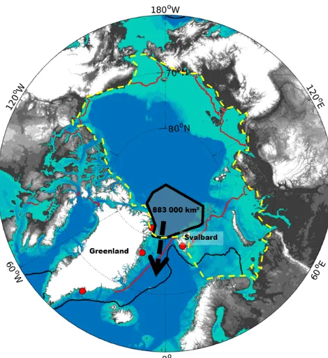
Figure 1.The Arctic Ocean and surrounding shelf and land areas. The large black arrow shows the location of Fram Strait, and the red circles show the positions of the meteorological stations with sea level pressure observations. The 1935–2014 mean positions of the mid-month sea ice extent are plotted for September (red) and March (black). The 1935–2014 mean annually exported sea ice area (883 000 km2) is illustrated by the polygon. The outer extent of the Arctic Ocean domain is drawn using the yellow dashed line.
and atmosphere (Graversen et al., 2011; Zhang, 2015), an increase in downwelling long-wave radiation due to cloud cover (Francis et al., 2005), and changes in atmospheric cir-culation that enhance ice export out of the Arctic (Nghiem et al., 2007; Smedsrud et al., 2011). However, despite the large number of existing studies, the role and influence of natu-ral variability remain unclear, especially on longer timescales than the current satellite data record.
Historically, about 10 % of the Arctic sea ice area is ex-ported through Fram Strait (FS) annually (Fig. 1), and the ice export through the other Arctic gateways is an order of mag-nitude smaller (Kwok, 2009). Because quite thick ice is lost by this export through FS (Hansen et al., 2013), a larger than normal ice export will decrease the remaining mean thick-ness within the Arctic Basin. An influence of export anoma-lies on Arctic sea ice thickness was previously suggested by Rigor et al. (2002) using buoy data. A similar conclusion was reached using model simulations from climate models participating in the Coupled Model Intercomparison Project Phase 5 (CMIP5) (Langehaug et al., 2013). Recently Fuˇckar et al. (2015) found that much of the northern hemispheric sea ice thickness variability could be explained by changes in sea ice motion related to wind forcing.
any significant change in FS ice volume export for the pe-riod 2003–2008 for observed winter means (October–April). Thus, some uncertainty remains on how FS ice export has changed and how it has influenced the long-term decline in the summer ice cover.
The Arctic seasonal maximum sea ice cover generally oc-curs in late February or early March (Zwally and Gloersen, 2008), though it has also been observed to occur as late as early April (e.g., on 2 April in 2010; https://nsidc.org/ arcticseaicenews/2010/04). Changes in ice export through FS between March and August could therefore influence the fol-lowing September SIE by fostering development of open wa-ter within the ice pack that in turn enhances the ice–albedo feedback during the melt season (Smedsrud et al., 2011; Kwok and Cunningham, 2010). Such an influence has re-cently been examined between 1993 and 2012 by Williams et al. (2016) in combination with coastal divergence. This study suggested that Fram Strait ice area export is a good predictor for the September sea ice extent because it repre-sents the sum of ice export from the peripheral seas and the net pack ice divergence. This study expands on the work by Williams et al. (2016) by estimating the FS ice area export over a much longer time period, from 1935 to 2014. In this study, we evaluate the long-term mean, variability, and trends over this 80-year record and further examine the influence of the long-term FS export on a new time series of September SIE, also covering the years 1935–2014 (Walsh et al., 2015).
2 Data and methods
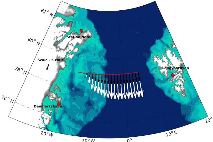
Figure 2.The Fram Strait between Greenland (left) and Svalbard (right) with summer (black arrows) and winter (white arrows) mean sea ice drift speed. Southward ice drift across 79◦N (red line) from February 2004 to December 2014 were interpolated to 1◦bins based on SAR imagery. Summer speeds are June–September means, while winter speeds are December–March means. Shades of blue show ocean bathymetry in 100 m steps down to 500 m depth. Red circles show locations for surface pressure observations on Svalbard (Longyearbyen) and Greenland (Station Nord and Danmarkshavn). Pressure observations were interpolated between the Greenland stations to calculate the mean pressure gradient along 78.25◦N. Before 1958 pressure observations from Danmarkshavn are lacking, so observations from Tasiilaq (65.60◦N, 37.63◦W) were used, further south along the Greenland coast (Fig. 1).
2.1 Ice drift observations: 2004–2014
We use observed sea ice drift speeds onwards from Febru-ary 2004 and updated through December 2014, calcu-lated by recognizing displacement vectors manually on ASAR WideSwath and Radarsat-2 ScanSAR images cap-tured 3 days apart (Kloster and Sandven, 2015). These im-ages were resampled from 50 to 100 to 300–500 m pixels in order to reduce the SAR speckle noise, greatly improving feature recognition and tracking accuracy over the 3-day time interval. Displacement vectors that cross 79◦N were linearly interpolated to bins (1◦ longitude, each 21 km) from 15◦W to 5◦E (Fig. 2).
For most 3-day image pairs, displacement vectors with an accuracy of±2 km and spacing of 30–50 km were calculated using the known satellite orbit and one reference point. Drift-ing platforms and buoys were used to estimate uncertainties, indicating values better than±3 %. This accuracy is consid-ered sufficient because subsequent averaging or addition in time–space of many unbiased vectors will generally result in improved accuracy. We calculated mean cross-strait ice drift speed values, defined as the spatial–temporal mean south-ward speed of all ice crossing 79◦N (Fig. 1) between the fast ice edge and the pack ice edge at 50 % sea ice concentration. On the western side of the strait, a linear interpolation from zero motion in the stable fast ice to the first measured
mo-tion vector was made. It was assumed that ice displacement to the east of the last measured vector is constant near the ice edge. The monthly mean speed value results from the aver-aging of about 50 individual, unbiased displacement vectors, and thus the calculated mean speed value should have an ac-curacy better than±0.1 cm s−1.
Using the 3-day mean drift speeds as derived above, cor-responding FS ice area export along 79◦N was calculated as the product of this sea ice drift and corresponding 3-day values of passive microwave sea ice concentration (Kloster and Sandven, 2015). The combined uncertainty of the pas-sive microwave sea ice concentration and ice speed is about
±5 % in the 3-day fluxes. The monthly mean values from 2004 to 2014 are shown in Fig. 3. Values are summarized over a month or a season here (cumulative values) and the uncertainty for these values are further reduced because un-certainties become lower with a larger number of samples. A spring ice area export value of 500 000 km2is the sum of 60 3-day values from 1 March to 31 August and has an esti-mated uncertainty better than±5000 km2. From here on, ice area export will be referred to as ice export.
2.2 Sea level pressure observations: 1935–2014
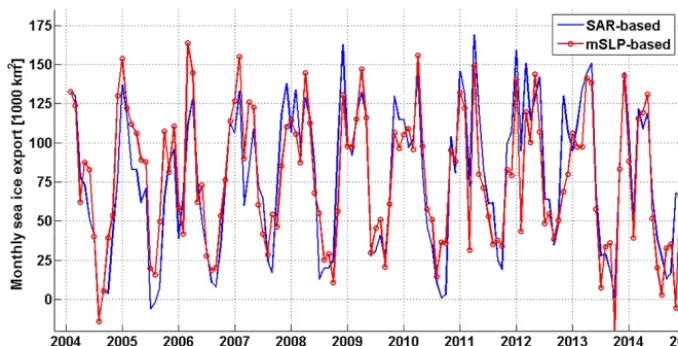
Figure 3.Monthly mean Fram Strait sea ice export. The SAR-based values are calculated from 3-day displacement vectors and corresponding sea ice concentration, while the other time series uses observed mean sea level pressure (mSLP) and the seasonal correction for a stronger East Greenland current during winter.
to the ASAR data starting in February 2004. The cross-strait difference along 78◦N was calculated between 18◦W and 15◦E based on monthly mSLP observations from Longyear-byen (Fig. 2, Svalbard Airport, Norwegian Meteorological Institute, http://eklima.met.no) and from weighted averages of monthly mSLP from two nearby stations on the Green-land side at 18◦W: Danmarkshavn and Nord (Fig. 2, Danish Meteorological Institute, Cappelen, 2014). mSLP is available from Danmarkshavn and Nord back to 1958. For the 1935– 1958 period, a linear regression between Nord and Tasiilaq further south was performed.
The mSLP observations were then used to calculate cross-strait geostrophic winds following Thorndike and Colony (1982). Because mSLP from Danmarkshavn and Nord corre-lated well (r=0.93), we derived a linearly interpolated value at 78◦N, 18◦W directly using these stations onwards from 1958. For the period 1935–1958, interpolated values between station Nord and Tasiilaq were used, which have a somewhat lower correlation (r=0.77). Our method assumes that wind and ocean drag are the dominant forces acting on the sea ice, consistent with geostrophic winds explaining more than 70 % of the variance of ice drift speed in the Arctic Ocean (Thorndike and Colony, 1982). In the FS, winds have also been found to be the dominant force acting on sea ice (Widell et al., 2003), and the cross-strait pressure difference in SLP well represents the ice drift on a daily timescale (Tsukernik et al., 2010). However, van Angelen et al. (2011) simulated local Fram Strait surface winds and found them more related to thermal wind forcing than larger-scale forcing. Neverthe-less, they found that ice export for individual years from 1979 to 2007 was better explained by large-scale forcing because thermal winds were mostly constant between years.
2.3 Merged ice drift and export: 1935–2014
We next evaluate the relationship between the observed SAR ice drift speed and the geostrophic wind since 2004 to ver-ify the use of mSLP to extend the record prior to 2004. A linear regression between monthly mean ice drift speed and geostrophic wind from 2004 to 2014 (r=0.77, with 95 % confidence interval [0.68, 0.83]) reveals that the ice in FS generally drifts at a speed that is 1.6 % of the geostrophic wind speed (Eq. 1). The constant contribution resulting from the linear regression represents the speed of the ice given no local wind forcing and is 6.7 cm s−1(Eq. 1). In other words, the value of 6.7 cm s−1 represents the mean ocean current, though nonlinear components of ice drift, including forces from variations in ocean currents or internal ice stress, may also represent parts of this constant (Thorndike and Colony, 1982). It is important to note, however, that it is not the lo-cally wind-driven ocean current. Both the mean drift speed and the mean ocean current are comparable to previous stud-ies (Widell et al., 2003; Smedsrud et al., 2011; Thorndike and Colony, 1982). The standard error of the regression is 3.4 cm s−1.
Vice=0.016×Vg+0.067(m s−1) (1)
If sea ice concentration does not change systematically in-side the ice pack locally, we expect a similar relationship be-tween mSLP and sea ice export. This was indeed what we found, with a correlation between the cross-strait mSLP and ice export ofr=0.73.
Jan Feb Mar Apr May Jun Jul Aug Sep Oct Nov Dec 0
5 10 15 20 25
Month
Ice drift speed [cm s ]
SAR mSLP−based mSLP−based corrected
–1
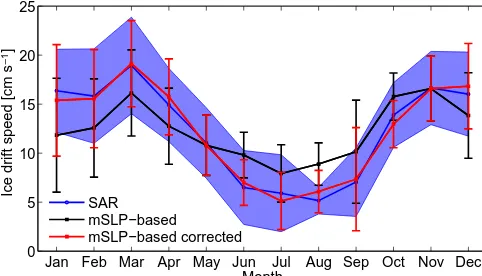
Figure 4.Annual cycle of monthly mean southward ice drift speed in Fram Strait between 2004 and 2014. Observed ice drift speed (SAR) are shown in blue, and our pressure-based ice drift speed in black. The corrected ice drift speed is shown in red. Standard devi-ations of observed ice drift speed are shaded in purple, and those of calculated ice drift speed as vertical colored lines.
However, a clear seasonal difference is observed be-tween the SAR ice speed and the mSLP-estimated ice speed (Fig. 4). Previously it was assumed that the mean ocean cur-rent would be constant throughout the year (Kwok, 2009; Smedsrud et al., 2011), e.g., 6.7 cm s−1from Eq. (1). How-ever, based on the 10 years of detailed SAR velocities, we instead find it is necessary to account for the seasonality of the mean ocean current in order to match the mSLP-derived ice drift with the SAR data. The suggested seasonal change is a mean winter current (December–April) of 9.5 cm s−1 and a mean summer current of 3.9 cm s−1 (June–October).
The East Greenland Current (EGC) thus appears 2.8 cm s−1
stronger than the mean during winter and 2.8 cm s−1weaker during summer. Note that this seasonal difference cannot be explained by a seasonally varying internal ice stress, because ice is thicker and denser during winter, which would result in a larger ice stress and therefore weaker ice drift speed for a similar wind speed.
An increase in the EGC would be consistent with gener-ally stronger winds in the North Atlantic region during win-ter, as well as stronger thermal forcing (van Angelen et al., 2011). This suggests that the EGC is responding to the larger-scale wind forcing as well as to the local winds. Generally, the entire circulation along the continental slope of the Arc-tic Basin–Nordic seas is driven by the wind stress curl north of the Greenland–Scotland ridge (Isachsen et al., 2003). Two recent studies confirm that the EGC is stronger during win-ter, and may respond to the large-scale wind stress curl in the Nordic Seas or the stronger thermal forcing during winter. It is thus likely that this increase is causing the additional win-ter export (Fig. 4). De Steur et al. (2014) analyzed mooring data along 79◦N between 1997 and 2009 and found that sur-face currents were below 5 cm s−1 during summer and 10– 15 cm s−1during winter, also varying in the east–west
direc-tion. Daniault et al. (2011) found a maximum in the flow in January and a minimum in July for the years 1992–2009 based on satellite radar altimetry data at 60◦N and that the vertical distribution remained constant over this time period. The above studies support a bias correction for the con-stant EGC speed in Eq. (1) to increase (decrease) the mSLP-based winter (summer) ice speeds. Thus, assuming a stronger EGC during winter, and weaker during summer, we added the seasonal difference to the time series of mSLP-based ice speed. This means that in Eq. (1), we add 2.8 cm s−1 to the constant 6.7 cm s−1for the months December through April, and subtract 2.8 cm s−1from the constant 6.7 cm s−1for June through October, while May and November remained un-changed. This bias-corrected mSLP-based ice speed better matches the SAR observations (Fig. 4), with a correlation of
r=0.88.
The same correction was also applied for the calculated ice export, representing a decrease in summer values of 23 800 km2and increase in winter values of 22 400 km2 ac-cordingly (not shown). The seasonal correction further im-proves the correlations between observed and mSLP-based ice export (r=0.87). Figure 3 compares the mSLP-based and SAR-based monthly mean ice export values between 2004 and 2014 and confirms the close agreement between them. The mSLP-based time series slightly over and un-derestimates the observed SAR-based values for individual months, but there is no systematic difference over time.
In other words, we expect our bias-corrected mSLP-based time series from 1935 to 2004 to explain about 80 % of the “true” ice drift and export variability. Note that we have as-sumed a constant seasonality for this bias correction and that if changes in seasonality for ice drift exist prior to 2004 ex-ist this would affect our results. Using high-resolution wind simulation, van Angelen et al. (2011) found a similar correla-tion (r=0.85) between annual export and surface wind for 1979–2007. Our described seasonal correction is also con-sistent with their simulated stronger thermal forcing during winter that would set up a sea surface gradient and drive a related stronger barotropic ocean current.
Taking into account the seasonally varying EGC and ther-mal wind explained above, in addition to the monthly vary-ing geostrophic winds based on observed mSLP, we calculate monthly mean ice export prior to 2004 and merge them with the SAR-based observed ice export from 2004 to 2014. This generates an 80-year-long record of monthly mean FS ice ex-port.
2.4 Sea ice extent
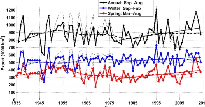
pro-Figure 5.Southward ice area export in Fram Strait. Ice export from 1935 to 2003 is based on the relationship between observed mean sea level pressure and observed ice export by SAR, and ice export from 2004 to 2014 is solely the observations by SAR. Annual values (black) are averaged for 1 September through 31 August. Winter export is 1 September–28 February (blue) and Spring is 1 March–31 August (red). Values are plotted half way through the respective period. Smoothed time series are included produced by filtering with a 20-year-cutoff eighth-order Butterworth filter (thick dash-dotted lines), and linear trends are plotted onwards from 1979. The long-term (1935–2014) trends are not included because they are not significantly different from zero. The effect of using a time-varying seasonal sea ice concentration based on Walsh et al. (2015) is shown using thin dashed lines.
vides mid-month sea ice concentrations on a 0.25×0.25◦ grid (Walsh et al., 2017). A total of 16 different sources of information were used to construct ice cover informa-tion back to 1850. Prior to the modern satellite data record, which began in October 1978 from a series of successive passive microwave sensors (e.g., the Scanning Multichannel Microwave Radiometer (SMMR) and several Special Sen-sor Microwave/Imager (SSM/I) and SSMIS senSen-sors), ob-servations come from earlier satellite missions, aircraft and ship observations, compilations by naval oceanographers, ice charts from national ice services, and whaling log records, among others. For many regions and time periods several sources of sea ice data and weighting was applied (Walsh et al., 2017). The monthly files are intended to represent ice on the 15 or 16 of each month using the NASA Team sea ice algorithm. Using this data set, the ice extent is defined as the area covered by ice of greater than 15 % ice concentration.
Initial evaluation of the data set indicated a problem with inconsistencies in the land mask applied throughout the en-tire time period. This was fixed and led to a slight reduc-tion in the overall sea ice extent prior to the satellite data record. To evaluate how ice export influences changes in sea ice cover within the Arctic Basin, we use an Arctic Ocean domain mask as defined in Serreze et al. (2007) and com-pute sea ice extent within this domain only (Fig. 1). For the September SIE time series this mainly excluded the Green-land Sea downstream of the FS ice export, where we expect high export to contribute to a larger ice cover.
The mid-month sea ice concentration from Walsh et al. (2015) along 79◦N (15◦W to 5◦E) was also used to
ex-amine the influence of changing sea ice concentration on the spring and winter FS ice export (Fig. 5). This influence is overall smaller than±10 %, and onwards from 1979 no sig-nificant differences are visible. We have chosen to present ice export based solely on the station-based daily SLP obser-vations producing the monthly mean mSLP, as further dis-cussed below.
3 Results
3.1 Long-term (1935–2014) annual mean ice export variability and trends
Figure 2 shows that the temporal mean ice drift speed is quite constant spatially across the FS eastward of 5◦W and that the speed decreases westward towards the Greenland coast. Velocities are clearly strongest during winter with mean speeds above 20 cm s−1, decreasing to less than 10 cm s−1 during summer eastward of 5◦W. FS ice drift is in the south-southwesterly direction steered by the Greenland Coast. The ice export occurs mostly between 5◦W and the Greenwich meridian. The export is limited on the western side by the decreasing ice speed, reaching zero at 16◦W, where station-ary land fast ice is usually found. On the eastern side the ice export is limited by zero concentration, varying from 5◦W to 5◦E (not shown).
has a long-term mean of 528 000 km2. We define spring export as March through August, and the mean value is 354 000 km2. Note that the 1935–2014 long-term annual mean ice export of 883 000 km2 is 25 % higher than previ-ously found by Kwok (2009) using data from 1979 to 2007, but similar to values from Thorndike and Colony (1984) and Widell et al. (2003) for 1950–2000 and Smedsrud et al. (2011) for the period 1957–2011.
The consequences of the export variability are discussed later; here we just note that since 2006 ice export has re-mained higher than the long-term mean (Fig. 5) and that for 2011–2013 the annual export exceeded 1 million km2. In ad-dition, there are a number of notable export events in the 80-year time series. Note that there are no mSLP values ob-served during World War II, so the seemingly constant values from 1940 to 1945 are set identically to the long-term mean annual values. The lowest annual export occurred in 1946 with only 599 000 km2exported, and the highest export with 1 206 000 km2was in 1995.
The annual and seasonal trends appear robust, and no sys-tematic difference appears by merging the mSLP-based val-ues prior to 2004 with the SAR-based valval-ues since 2004. This was confirmed by comparing trends for the merged time series (1935–2014) with those based on the observed mSLP only (1935–2014). For example, the mSLP-based an-nual trend is 0.2 versus 0.3 % per decade for the merged values, while for winter the values are 1.1 versus 1.6 % per decade and for spring−0.8 versus−1.3 % per decade. These long-term trends are small and not significantly different from zero (p=0.2), and they are therefore not included in Fig. 5. We also searched for specific cycles, or frequencies, in the new 80-year time series. Apart from the obvious annual cycle (Fig. 4) we could not find any special peaks in calcu-lated spectrums of the annual, winter, or spring export (not shown). The smoothed time series appeared similar for cutoff frequencies representing cycles above 10 years, so we chose to show a 20-year cutoff (or frequency of 0.05 cycles yr−1) in Fig. 5. Overall the variations are similar for the annual and spring export values, while there is less long-term variabil-ity in the winter export. For the smoothed series there is a distinct peak in annual and spring export between 1951 and 1954. After 1954, there is a decrease in annual and spring export until the mid-1980s, and an overall increase onwards to 2014. Thus, there is a hint of a long-term multidecadal oscillation with a period around 70 years.
3.2 Recent (1979–2014) ice export variability and trends
The increasing exports onwards from the 1980s create sta-tistically significant positive trends for both the annual and seasonal values over the modern satellite data record and the time period for which large declines in sea ice have been ob-served. For example, from 1979 to 2014 we find a positive trend in annual export of +5.9 % (p=0.025) per decade
(Fig. 5). This trend is consistent with a general increase in ice drift speed observed well inside the deep Arctic Basin (Fig. 1, Spreen et al., 2011; Rampal et al., 2009), but the small number of buoys exiting in FS have precluded estimat-ing trends there. The positive trend in annual ice export from 1979 to 2014 is largely driven by higher ice export during spring: the winter ice export trend is+3.0 % (p=0.213) per decade, while the spring export trend is+11.1 % (p=0.011) per decade (Fig. 5).
The increasing spring export since 1979 may have im-portant implications for the sea ice cover, and we there-fore analyze this time period further to make sure no bi-ases are introduced by using the merged mSLP+SAR export fields. Trends are found to be similar between the merged (mSLP+SAR) and mSLP-based time series, caused by the very similar monthly values between 2004 and 2014 (Fig. 3). There is a positive trend in spring export of 13.1 % (±6.8) per decade from the mSLP-based estimates and a trend of 11.1 % (±8.1) per decade using the merged time series. These trends are not significantly different at the 95 % confidence level. Note that, around 1980, the spring export was approximately half of the winter export. The robust trend in spring export since 1980 has resulted in a smaller seasonal difference, and for 2011 and 2012 the export in winter and spring were of similar magnitude (Fig. 5). The recent high values could per-haps be surprising, were it not for the longer time series where a similar high spring export is evident in the 1950s.
We also do not find a “shift” in the trends after 2004 when the SAR values are used. For example, the spring 1979– 2003 trend is+9.1 % (±11.3) per decade, almost as high as the 11.1 % for the 1979–2014 period. So the spring export is the main cause of increased annual export before and af-ter 2003, and the differences are not significant at the 95 % confidence level. Due to the few years and large variability, the ∼20-year trends are generally not significantly differ-ent from zero (p>0.05). The annual trend for 1979–2003 is 3.8 % (p=0.36), compared to 5.9 % for 1979–2014, and for winter 0.8 % (p=0.84), compared to 2.6 % for 1979–2014. This indicates that the export trends since 1979 are related to a gradual increase in mSLP across FS over most of this period. The increased spring ice export is due to stronger geostrophic winds, driven by an increase of 0.53 hPa per decade in mSLP over Greenland between 1979 and 2014. The increase in SLP is strongest in June–August and covers the larger part of Greenland (not shown). The mSLP trend on the Svalbard side is a slightly lower and negative trend, is strongest in March–May, and covers the larger part of the Barents Sea (not shown).
4 Discussion
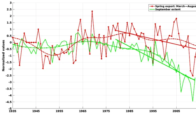
Ange-Figure 6.Spring Fram Strait ice area export (red) and mid-September Arctic SIE (green). The ice export is averaged for March 1st through 31 August. Both time series have been normalized by subtracting the mean and dividing with the standard deviation. The ice export is here plotted with negative values as high southward export for easier comparison. Smoothed time series are included, produced by filtering with a 20-year-cutoff eighth-order Butterworth filter. The 1979–2014 trends in ice export and mid-September SIE are shown as solid straight lines. SIE values are obtained from Walsh et al. (2015).
len et al., 2011), because we discovered unexplained system-atic differences between NCEP reanalysis mSLP fields and observed mSLP within the FS in recent years. Despite the wide use of reanalysis data sets, they are heavily influenced by the numerical model used to simulate the fields, and they are therefore regarded as less accurate than the station data used in this study.
Prior to 2004 we do not utilize observations of cross-strait variations in the width of the ice-covered area, ice speed, or ice concentrations, but base our ice export values solely on the regression equation found between observed mSLP from Longyearbyen, station Nord, Danmarkshavn, and Tasi-ilaq (Fig. 2) and observed SAR ice export. The new Walsh et al. (2015) mid-month sea ice concentration provided a possi-bility to consistently analyze the effect of varying seasonal sea ice concentration prior to 2004 (Fig. 5). The changes were overall small, and only during the 1950s were sea ice concentration anomalies across 79◦N (15◦W–5◦E) large enough to contribute to a 10 % increase in ice export (Fig. 5). The 1935–2013 seasonal mean ice concentration from Walsh et al. (2015) during winter is 83 % (standard devia-tion of±11 %) and for spring is close to 72 % (standard de-viation of±9 %, not shown). There are no significant long-term trends in sea ice concentration for the spring or win-ter months between 1935 and 2013. We concluded that using mSLP based on daily observations is the most consistent way to calculate ice export over the last 80 years. The Walsh et al. (2015) values are mid-month values mostly based on sea
ice extent estimates during summer before 1979, with very few winter observations available.
There are other possible systematic contributions to the overall uncertainty from a number of factors, like sea ice roughness, the ocean current, the thermal wind, and changes in sea ice thickness. Our best estimate for the uncer-tainty in the seasonal spring and winter means is therefore about 10 %, i.e., 354 000 km2±35 000 km2 for spring and 528 000 km2±52 000 km2for winter.
4.1 Long-term variability of September SIE
The mid-September SIE time series shows two stages, a modest increase from 1935 until around 1965 and then a monotonic decrease over the last 50 years (Fig. 6). There is a “break point” around the mid-1990s when the September SIE loss accelerates as has been noted earlier (Stroeve et al., 2012). From the mid-1960s until the mid-1990s the loss in SIE is small. The minimum SIE value predating 1995 occurs in 1952, and the last two minima in 2007 and 2012 are also clearly visible (Fig. 6). The overall mid-September SIE max-imum occurred in 1963.
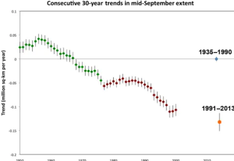
con-Figure 7.Consecutive 30-year trends of mid-September SIE in the Arctic Basin. The first green symbol shows the 30-year trend be-tween 1935 and 1964 and is plotted at the center year in 1950. The next value in 1951 shows the trend for 1936–1965, and so on. The last green symbol in 1975 is for the 1961–1990 trend. The red sym-bols show trends after 1990, ending with the 1984–2013 trend. The blue symbol shows that the 1935–1990 trend was zero, and the or-ange symbol shows the trend from 1991 to 2013. SIE values are obtained from Walsh et al. (2015).
secutive 30-year trends are significantly different from trend periods before 1990 (Fig. 7), and thus the September ice loss since the 1990s is unprecedented as far back as 1850 (Walsh et al., 2017).
4.2 Effects of long-term variability and trends in ice export
Our ice export values are largely consistent with previous studies on FS ice export for the recent decades (Kwok et al., 2013; Spreen et al., 2009; Smedsrud et al., 2011). The year-to-year variability is of the same order, and the maximum and minimum values are also similar. The largest difference to the Smedsrud et al. (2011) export values is that the time se-ries is updated to 2014 and now extends back to 1935 and the seasonal adjustment representing the EGC provides a better match with the SAR-based monthly export (Fig. 3). In ad-dition, there is no overall long-term linear trend in annual export.
The effect of sea ice drift variability on the Arctic sea ice cover in general has been recognized for a long time (Thorndike and Colony 1982). Rigor et al. (2002) used drift-ing buoy data from 1979 to 1998 and found a systematic change between the 1980s and 1990s driven by the large-scale atmospheric forcing. During the 1980s the Beaufort gyre was large, the ice stayed inside the Arctic Basin for sev-eral years, and FS sea ice export was low, contributing to a thicker ice cover. In the 1990s the Beaufort gyre weakened, ice drift was more directly from the Siberian coast to FS, and the FS sea ice export was higher. Our results are
con-sistent with Rigor et al. (2002) in that the annual export was lower during the 1980s (810 000 km2) than during the 1990s (890 000 km2). The overall maximum annual export in a cal-endar year occurred in 2012 with a value of 1 176 000 km2, but the second largest calendar year export occurred in 1995 (1 131 000 km2). Note that these values are a little different from those plotted in Fig. 5, which show the winter+spring export from 1 September through 31 August.
One suggested mechanism for the rapid decline in summer Arctic SIE is that a larger winter export could create a larger fraction of thin first-year ice that is more prone to melting out the following summer. In addition, first-year ice is smoother than thick and old ice and may allow for larger fractions of melt ponds during summer (Landy et al., 2015). Schröder et al. (2014) found a strong correlation between such simu-lated spring melt pond fractions and September Arctic SIE. However, in this study we find that the correlation between winter ice export and the following September SIE is mod-est (r= −0.26 between 1979 and 2014). Thus, the small in-crease in winter ice export over the last 35 years (2.6 % per decade) suggests that summer ice loss is not particularly sen-sitive to winter sea ice export. Because the winter export is larger than the spring export there has generally been a clear connection between annual and winter export anoma-lies. However, while there is little change in winter export, there has been a notable increase in the spring export. In fact, in recent years the spring export has been almost as large as the winter export (Fig. 5). An increase in summer ice ex-port (June–September) for 2000–2010 was already noted by Kwok et al. (2013), and here we show that this is part of a longer trend. We turn our attention towards the increasing spring export in Sect. 4.5, but first examine the cause of the variability in the larger atmospheric circulation.
4.3 Influence of large-scale atmospheric circulation
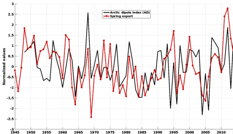
Figure 8.Fram Strait spring export (March–August) and April–July Arctic dipole (NCEP/NCAR reanalysis) anomalies from 1948 to 2014. Both time series are detrended and normalized by their standard deviations, 0.817 million km2and 28.8 hPa, respectively. The correlation between them isrAD-FS ice export=0.45 for the entire period and similar for 1979–2014(rAD-FS ice export=0.44).
no correlation between the winter North Atlantic Oscillation index (NAO, which closely resembles the AO), and winter FS ice export for the period 1958–1977, but did find higher correlations for 1978–1997, again consistent with Rigor et al. (2002).
Other studies have suggested that FS export is more strongly linked to a SLP dipole pattern than the AO (Tsuk-ernik et al., 2010). They found that on a daily timescale the atmospheric circulation pattern responsible for the ex-port anomalies from 1979 to 2006 was a dipole between the Barents Sea (low pressure) and Greenland (high pres-sure). The ice motion was maximized at 0 lag, persisted year-round, over timescales of 10–60 days. This SLP dipole pat-tern emerged from the second empirical orthogonal function (EOF) of daily SLP anomalies in both winter and summer, with maximum correlation east and west of the FS. An im-plication of this result is to use station-based observed cross-strait SLP pressure gradient like we have done here.
The observed cross-strait SLP gradient, the dipole pat-tern analyzed by Tsukernik et al. (2010), and the Arctic dipole (AD) are similar expressions of varying strength of the southerly winds in FS (Wu et al., 2006). The AD has been suggested previously as a major driver of the record low Arctic summer SIE in 2007 (Wang et al., 2009) and was defined as the second leading mode (PC2) of spring (April– July) SLP anomalies within the Arctic Circle. In this study, we define a positive AD pattern as having a positive SLP anomaly over Greenland and a negative SLP anomaly over the Kara and Laptev seas, a pattern which enhances transpo-lar ice drift. We calculate the AD index onwards from 1948
using the NCEP/NCAR reanalysis data, for which data are not available before 1948. The observed AD index and spring export correlates (rAD-FS ice export=0.45)over the longer pe-riod 1948–2014 (Fig. 8), as well as over the shorter satellite data record (rAD-FS ice export=0.44 for 1979–2014). These correlations suggest that the AD explains part of the FS ice export variability but that the cross-strait SLP gradient re-mains the best predictor of the local wind forcing and there-fore FS sea ice drift. These results substantiate the results of Wu et al. (2006) that found a similar link for FS ice mo-tion and the AD using buoy data from 1979 to 1998. In fu-ture projections, high rates of summer Arctic sea ice loss are also associated with enhanced transpolar drift and FS ice ex-port driven by changing sea level pressure patterns (Wettstein et al., 2014). Wettstein at al. (2014) found co-varying atmo-spheric circulation patterns resembling the AD, with maxi-mum amplitude between April and July.
4.4 High annual export during the last decade
dif-ference between previous passive microwave-based export values (Kwok, 2009) and our results. Note that Kwok et al. (2013) do find a positive trend for annual export for 2001– 2009, and the values are lower. We believe that the cause of the differences primarily results from the coarse resolution of the passive satellite observations missing some high-speed export events during winter. We speculate that high sea ice concentrations in the FS make it difficult to track individual sea ice floes using the coarser-resolution passive microwave images as done by Kwok et al. (2013) and note that changes in FS sea ice concentration between 1979 and 2004 do not lead to such differences in ice export (Fig. 5).
The Arctic Basin covers an area of about 7.8 million km2 and has been fully ice covered from November through May since 1979. The annual ice export during the 1980s (∼800 000 km2) was 10 % of this winter ice-covered area. However, during the last 7 years (2007–2014) the mean an-nual ice export increased to nearly 1 million km2, represent-ing 13 % of this area. This is the relative ice export, or the large-scale divergence of the Arctic Basin sea ice cover: the export divided by the area covered by sea ice.
If the sea ice cover decreases and the export remains con-stant, the divergence, or the relative export, increases too. The observed increase in export represents a 30 % increase in the relative area export, but with a smaller annual mean ice-covered area inside the Arctic Basin the increase rises to about 40 %. This value is based on using a 1 million km2 ex-port and a mean annual ice-covered area inside the Arctic Basin of 7.0 million km2for the last 7 years (2007–2014). Such an increase in export is expected to contribute towards both a thinner and smaller Arctic ice cover in general (Lange-haug et al., 2013), because older and thicker sea ice than the Arctic Basin average is transported southward through FS. During winter, the open water anomalies created within the basin quickly refreeze, and thus an impact of the modestly increased winter ice export since 1979 has likely been to-wards a thinner ice cover (Lindsay and Schweiger, 2016). This is consistent with Fuˇckar et al. (2015) who found that a reduction of the FS winter export related to their Canadian– Siberian dipole cluster explains a thickening over most of the Arctic Basin between 0.2 and 0.5 m. This cluster is the one with the largest change in FS export and explains 28.6 % of the variability, while the other two clusters mostly describe divergence within the basin. Williams et al. (2016) recently found a clear link between FS area export anomalies and September SIE (r=0.72) for the years 1993–2014 and that export anomalies from February until June contributed to the following September SIE. We therefore proceed with a dis-cussion of the spring export that has increased since 1979.
4.5 Consequences of spring Fram Strait ice export anomalies
The later in the season the export anomaly occurs, the stronger effect one might expect on the September minimum
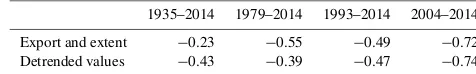
Table 1.Correlations over time between Fram Strait spring export and mid-September sea ice extent (rFS ice export-Sept SIE).
1935–2014 1979–2014 1993–2014 2004–2014 Export and extent −0.23 −0.55 −0.49 −0.72 Detrended values −0.43 −0.39 −0.47 −0.74
SIE. However, working against this is the overall decrease in export from March towards August (Fig. 4). However, even if there is some regrowth in March, April, and May from in-creased spring export, the newly formed ice will be thin and have a thin snow cover and therefore likely melt more easily and deform later the same season. The transition from win-ter and refreezing to summer and positive ice–albedo feed-back occurs gradually later in the year as one moves north, but melting will prevail over most of the Arctic Basin on-wards from May (Markus et al., 2009). Williams et al. (2016) found that FS export anomalies are a better predictor for the September SIE than coastal divergence between 1993 and 2014. This was caused by the ice export being a good es-timate also for the net perennial pack ice divergence. Our re-sults confirm their findings for the last 2 decades, but we also find a more moderate link for the entire 80-year period. For the recent 10 years (2004–2014), when our ice export values are directly observed by SAR the detrended anticorrelation is
rFS ice export-Sept SIE= −0.74 (Table 1), similar to Williams et al. (2016). For the last 20 years we get a more modest in-fluence (r= −0.47), and for the entire 80-year period we get
r= −0.43 (Table 1). The explained general variance is thus in the range 15–20 %.
The increase in spring FS ice export from the 1980s to 2010 was on the order of 200 000 km2 (Fig. 5). Mean-while the September SIE decreased by about 2.0 million km2 (Fig. 6). It is thus a similar magnitude of influence, about 10 %, between the direct change in spring FS ice export compared to the anomalies in September SIE themselves, as found based on the anticorrelations in Table 1.
Perovich, 2015), while the influence from atmospheric and oceanic heat transport is further discussed below.
Using coupled climate model simulations, Zhang (2015) identified the northward Atlantic heat transport, Pacific heat transport, and the spring AD as the main predictors of low-frequency variability of summer Arctic SIE. The study fo-cused on variability longer than 30 years and used a 3600-year segment of the preindustrial control simulation from the Geophysical Fluid Dynamics Laboratory (GFDL) Coupled Model version 2.1 (CM2.1). The influence of oceanic heat transport is smaller for the year-to-year variability that we focus on in this paper, leaving the AD as one of the main causes of simulated summer Arctic SIE variability at the in-terannual timescale.
Using the same 3600-year-long GFDL CM2.1 control sim-ulation, we find that the simulated spring FS ice export is indeed significantly inversely correlated with the September SIE (r= −0.34) and positively correlated with the AD index (r=0.63, not shown). This is similar to the inverse corre-lation found between the observed detrended spring FS ice export and September SIE over the 80 years from 1935 to 2014 (r= −0.43, Table 1) and supports a general level of in-fluence from the spring FS ice export of around 10 % on the observed September SIE loss. The link between the AD and spring FS ice export appears stronger in model simulations than for the available observations (rAD-FS ice export=0.45)
between 1948 and 2014.
The simulations in Zhang (2015) suggested the AD to be one of the main drivers of low-frequency sum-mer Arctic SIE. Here we would like to estimate how much of this AD influence can be explained by FS ice export at the interannual timescale from observed cor-relations since 1979. In this period rAD-Sept SIE= −0.53. We roughly estimate that 45 % of this correlation is caused indirectly by the FS spring export variability, becauser=rAD-FS ice export×rFS ice export-Sept SIE=0.44× −0.54= −0.24, and (−0.24)/(−0.53)=0.45. The FS spring export and the AD therefore have roughly equal con-tributions to September SIE variability in addition to the common mechanism being stronger northerly geostrophic
5 Conclusions
A new and updated time series of Fram Strait ice area ex-port from 1935 to 2014 was presented in this study. The new time series was constructed using high-resolution radar satel-lite imagery of sea ice drift across 79◦N from 2004 to 2014, regressed on the observed cross-strait surface pressure differ-ence back to 1935. The overall long-term mean annual export is 883 000 km2, and there are no significant trends over this 80-year record. Winter export (September–February) carries about 60 % of the annual export, while the spring export (March–August) carries the remaining 40 %.
The pressure difference from observed sea level pressure across the Fram Strait on Svalbard and Greenland directly explains 53 % of the variance in the observed ice export for 2004–2014. The best fit between ice drift and geostrophic winds results in a seasonal difference of∼3 cm s−1,
suggest-ing that the East Greenland Current, carrysuggest-ing a large part of the export, flows faster during winter and slower during sum-mer, consistent with generally stronger large-scale or ther-mal wind forcing. The ice export based on observed sea level pressure, including a seasonal variation in the underlying cur-rent, explains almost 80 % of the observed ice export vari-ance.
Despite not explaining all of the variance in ice export, the surface pressure-based time series suggest that about 18 % of the observed variance in September sea ice extent is ex-plained by spring ice export through Fram Strait between 1935 and 2014. The remaining 82 % of the variance would be caused by a large number of other processes, such as changes in ocean stratification and heat transport (Zhang, 2015), cloud cover (Francis et al., 2005), atmospheric heat transport (Graversen et al., 2011), and wind-driven ridging (Hutchings and Perovich, 2015). We have confidence in the moderate contribution from the Fram Strait export because it is a physical process, and the results are similar to simu-lations partially explaining the correlation between the ob-served AD anomalies and the September SIE (Zhang 2015). This is simply the wind forcing (AD) driving the ice export, again leading to anomalies in September SIE. Onwards from the 1990s, the covariance between Fram Strait spring ice area export and September SIE increases, consistent with the re-sults from Williams et al. (2016). Between 1993 and 2014, 22 % of the observed variance in mid-September sea ice ex-tent is explained by the spring ice export, increasing to 55 % for the last 10 years (Table 1). To reach such a level of in-fluence, feedbacks or other processes like ridging inside the basin and related coastal divergence have likely contributed and been correlated with the export anomalies (Williams et al., 2016). Positive feedback mechanisms enhancing summer SIE anomalies are the ice–albedo feedback and increased de-formation of thinner ice (Perovich et al., 2007; Rampal et al., 2009).
During the last 10–20 years, the Arctic sea ice cover has decreased quite rapidly, and the contributions from natural variability and greenhouse gas forcing are still being debated. We calculated an important driver of Arctic sea ice variability for the last 80 years and found that over this timescale there is no systematic increase in sea ice area exported southwards out of the Arctic Ocean in the Fram Strait. This is consis-tent with available historical simulations stating that we do not expect any systematic ice export change related to global warming (Langehaug et al., 2013). This is also consistent with studies stating that there is little systematic change in the Arctic large-scale circulation (Vihma, 2014). The Arctic ice cover is now thinner and more mobile than before, and over the last 3 decades the coupling between September ice cover and the Fram Strait spring sea ice area export has in-creased. The increased export over the last 35 years appears to be linked to natural variability on multi-decadal timescales because there is no trend over the last 80 years. Such a long-term variability has been found in northern hemispheric sur-face air temperature and temperature of inflowing Atlantic water to the Barents Sea (Smedsrud et al., 2013). Conse-quently we speculate that there may be potential for a par-tial recovery of the September SIE in the next decade or two, when, or if, the spring ice export decreases back to the long-term mean level of the last 80 years.
6 Data availability
The monthly mean 80-year time series of ice export is avail-able here: doi:10.1594/PANGAEA.868944.
Author contributions. Mari H. Halvorsen did most of the calcula-tions of sea ice export based on the sea level pressure data, Juli-enne C. Stroeve calculated and plotted sea ice extent variations and helped refocus the manuscript, Rong Zhang contributed with ana-lyzing the Arctic dipole time series and simulated sea ice export, and Kjell Kloster analyzed the original SAR images and calculated monthly mean ice speed and export. Lars H. Smedsrud prepared the manuscript with contributions from all co-authors and made most of the figures.
Acknowledgement. Sea ice drift data were obtained from Kloster and Sandven (2015), where ScanSAR data were provided by Norwegian Space Centre and Kongsberg Satellite Service un-der the Norwegian–Canadian Radarsat agreements 2012–2014. Observed pressure data are from the Norwegian and Danish meteorological institutes. The observed Arctic dipole index is derived from the NCEP/NCAR reanalysis. Mari H. Halvorsen was supported by the Geophysical Institute at the University of Bergen, Lars H. Smedsrud by the BASIC project in the Centre for Climate Dynamics (SKD) and the ice2ice project (ERC grant 610055) from the European Community’s Seventh Framework Programme (FP7/2007–2013), and Julienne C. Stroeve by NASA Award NNX11AF44G. We would like to thank Tor Gammelsrød, our editor Jennifer Hutchings, and the anonymous reviewers for helpful comments.
Edited by: J. Hutchings
Reviewed by: two anonymous referees
References
Björk, G. and Söderkvist, J.: Dependence of the Arctic Ocean ice thickness distribution on the poleward energy flux in the atmosphere, J. Geophys. Res.-Oceans, 107, 3173, doi:10.1029/2000JC000723, 2002.
Cappelen, J.: Weather observations from Greenland 1958–2013, Observation data with description, Tech. Rep., DMI Techni-cal Report 14-08, Danish MeteorologiTechni-cal Institute, Copenhagen, 2014.
Chapman, W. L. and Walsh, J. E.: Arctic and Southern Ocean Sea Ice Concentrations, Boulder, Colorado USA: National Snow and Ice Data Center, doi:10.7265/N5057CVT (last access: 20 Jan-uary 1996), 1991.
Comiso, J. C.: Large decadal decline of the Arctic multiyear ice cover, J. Clim., 25, 1176–1193, 2012.
Hakkinen, S., Proshutinsky, A., and Ashik, I.: Sea ice drift in the Arctic since the 1950s, Geophys. Res. Lett., 35, L19704, doi:10.1029/2008GL034791, 2008.
Hansen, E., Gerland, S., Granskog, M., Pavlova, O., Renner, A., Haapala, J., Løyning, T., and Tschudi, M.: Thinning of Arctic sea ice observed in Fram Strait: 1990–2011, J. Geophys. Res.-Oceans, 118, 5202–5221, doi:10.1002/jgrc.20393, 2013. Hilmer, M. and Jung, T.: Evidence for a recent change in the link
between the North Atlantic Oscillation and Arctic sea ice export, Geophys. Res. Lett., 27, 989–992, 2000.
Hutchings, J. K. and Perovich, D. K.: Preconditioning of the 2007 sea-ice melt in the eastern Beaufort Sea, Arctic Ocean, Ann. Glaciol., 56, 94–98, doi:10.3189/2015AoG69A006, 2015. Isachsen, P. E., La Casce, J., Mauritzen, C., and Häkkinen, S.:
Wind driven variability of the large-scale recirculating flow in the Nordic Seas and Arctic Ocean, J. Phys. Oceanogr., 33, 2534– 2550, 2003.
Kay, J. E., Holland, M. M., and Jahn, A.: Inter-annual to multi-decadal Arctic sea ice extent trends in a warming world, Geo-phys. Res. Lett., 38, L15708, doi:10.1029/2011GL048008, 2011. Kloster, K. and Sandven, S.: Ice Motion and Ice Area Flux in the Fram Strait at 79-81N, Technical Report, 322d, Nansen Environmental and Remote Sensing Center, Bergen, Norway, https://www.nersc.no/sites/www.nersc.no/files/ NERSC-TecRep-322d(2015).pdf, 2015.
Krumpen, T., Gerdes, R., Haas, C., Hendricks, S., Herber, A., Se-lyuzhenok, V., Smedsrud, L., and Spreen, G.: Recent summer sea ice thickness surveys in Fram Strait and associated ice vol-ume fluxes, The Cryosphere, 10, 523–534, doi:10.5194/tc-10-523-2016, 2016
Kwok, R.: Outflow of Arctic Ocean sea ice into the Greenland and Barents Seas: 1979–2007, J. Clim., 22, 2438–2457, 2009. Kwok, R. and Cunningham, G. F.: Contribution of melt in
the Beaufort Sea to the decline in Arctic multiyear sea ice coverage: 1993–2009, Geophys. Res. Lett., 37, L20501, doi:10.1029/2010GL044678, 2010.
Kwok, R., Spreen, G., and Pang, S.: Arctic sea ice circulation and drift speed: Decadal trends and ocean currents, J. Geophys. Res.-Oceans, 118, 2408–2425, 2013.
Landy, J. C., Ehn, J. K., and Barber, D. G.: Albedo feedback en-hanced by smoother Arctic sea ice, Geophys. Res. Lett., 42, 10714–10720, doi:10.1002/2015GL066712, 2015.
tic Ocean and adjacent seas, 1979–2005: Attribution and role in the icealbedo feedback, Geophys. Res. Lett., 34, L19505, doi:10.1029/2007GL031480, 2007.
Rampal, P., Weiss, J., and Marsan, D.: Positive trend in the mean speed and deformation rate of Arctic sea ice, 1979–2007, J. Geo-phys. Res., 114, C05013, doi:10.1029/2008JC005066, 2009. Rigor, I. G., Wallace, J. M., and Colony, R. L.: Response of Sea Ice
to the Arctic Oscillation, J. Clim., 15, 2648–2663, 2002. Schröder, D., Feltham, D. L., Flocco, D., and Tsamados, M.:
September Arctic sea-ice minimum predicted by spring melt-pond fraction, Nature Climate Change, 4, 353–357, 2014. Serreze, M. C., Barrett, A. P., Slater, A. J., Steele, M., Zhang, J., and
Trenberth, K. E.: The large-scale energy budget of the Arctic, J. Geophys. Res., 112, D11122, doi:10.1029/2006JD008230, 2007. Smedsrud, L. H., Sirevaag, A., Kloster, K., Sorteberg, A., and Sand-ven, S.: Recent wind driven high sea ice area export in the Fram Strait contributes to Arctic sea ice decline, The Cryosphere, 5, 821–829, doi:10.5194/tc-5-821-2011, 2011.
Smedsrud, L. H., Esau, I., Ingvaldsen, R.B., Eldevik, T., Haugan, P.M., Li, C., Lien, V. S., Olsen, A., Omar, A. M., Otterå, O. H., Risebrobakken, B., Sandø, A. B., Semenov, V. A., and Sorokina, S. A.: The role of the Barents Sea in the Arctic climate system, Rev. Geophys., 51, 415–449, doi:10.1002/rog.20017, 2013. Spreen, G., Kern, S., Stammer, D., and Hansen, E.: Fram
Strait sea ice volume export estimated between 2003 and 2008 from satellite data, Geophys. Res. Lett., 36, L19502, doi:10.1029/2009GL039591, 2009.
Spreen, G., Kwok, R., and Menemenlis, D.: Trends in Arctic sea ice drift and role of wind forcing: 1992–2009, Geophys. Res. Lett., 38, L19502, doi:10.1029/2009GL039591, 2011.
Stroeve, J. C., Kattsov, V., Barrett, A., Serreze, M., Pavlova, T., Holland, M., and Meier, W. N.: Trends in Arctic sea ice extent from CMIP5, CMIP3 and observations, Geoph. Res. Lett., 39, L16502, doi:10.1029/2012GL052676, 2012.
Stroeve, J. C., Markus, T., Boisvert, L., Miller J., and Bar-rett, A.: Changes in Arctic melt season and implications for sea ice loss, Geophys. Res. Lett., 41, 1216–1225, doi:10.1002/2013GL058951, 2014.
Thorndike, A. and Colony, R.: Sea ice motion in response to geostrophic winds, J. Geophys. Res.-Oceans, 87, 5845–5852, 1982.
Tsukernik, M., Deser, C., Alexander M., and Tomas, R.: Atmo-spheric forcing of Fram Strait sea ice export: a closer look, Clim. Dynam., 35, 1349–1360, doi:10.1007/s00382-009-0647-z, 2010. van Angelen, J. H., van den Broeke, M. R., and Kwok, R.: The Greenland Sea Jet: A mechanism for wind-driven sea ice ex-port through Fram Strait, Geophys. Res. Lett., 38, L12805, doi:10.1029/2011GL047837, 2011.
Vihma, T.: Effects of Arctic Sea Ice Decline on Weather and Climate: A Review, Surv. Geophys., 35, 1175–1214, doi:10.1007/s10712-014-9284-0, 2014.
Walsh, J. E., Chapman, W. L., and Fetterer, F.: Gridded monthly sea ice extent and concentration, 1850 onwards, Boulder, Colorado USA, National Snow and Ice Data Center, Digital media, 2015. Walsh, J. E., Fetterer, F., Scott Stewart, J., and Chapman, W. L.: A
database for depicting Arctic sea ice variations back to 1850, Ge-ogr. Rev., 107, 89–107, doi:10.1111/j.1931-0846.2016.12195.x, 2017.
Wang, J., Zhang, J., Watanabe, E., Ikeda, M., Mizobata, K., Walsh, J. E., Bai, X., and Wu, B.: Is the Dipole Anomaly a major driver to record lows in Arctic summer sea ice extent?, Geophys. Res. Lett., 36, L05706, doi:10.1029/2008GL036706, 2009.
Wettstein, J. J. and Deser, C.: Internal variability in projections of twenty-first-century Arctic sea ice loss: Role of the large-scale atmospheric circulation, J. Clim., 27, 527–550, 2014.
Widell, K., Østerhus, S., and Gammelsrød, T.: Sea ice velocity in the Fram Strait monitored by moored instruments, Geophys. Res. Lett., 30, 1982, doi:10.1029/2003GL018119, 2003.
Williams, J. Tremblay, B., and Newton, R.: Dynamic precondition-ing of the September sea-ice extent minimum, J. Clim., 29, 5879– 5891, doi:10.1175/JCLI-D-15-0515.1, 2016.
Wu, B., Wang, J., and Walsh, J. E.: Dipole anomaly in the win-ter Arctic atmosphere and its association with sea ice motion, J. Clim., 19, 210–225, 2016.
Zhang, R.: Mechanisms for low-frequency variability of summer Arctic sea ice extent, P. Natl. Acad. Sci. USA, 112, 4570–4575, 2015.
Zwally, H. J. and Gloersen, P.: Arctic sea ice surviving the summer melt: interannual variability and decreasing trend, J. Glaciol., 54, 279–296, 2008.