www.atmos-meas-tech.net/9/753/2016/ doi:10.5194/amt-9-753-2016
© Author(s) 2016. CC Attribution 3.0 License.
From pixels to patches: a cloud classification method based on
a bag of micro-structures
Qingyong Li1, Zhen Zhang1, Weitao Lu2, Jun Yang2, Ying Ma2, and Wen Yao2
1Beijing Key Lab of Transportation Data Analysis and Mining, Beijing Jiaotong University, Beijing, 100044, China 2State Key Laboratory of Severe Weather, Chinese Academy of Meteorological Sciences, Beijing, 100081, China Correspondence to: Qingyong Li ([email protected]) and Weitao Lu ([email protected])
Received: 6 July 2015 – Published in Atmos. Meas. Tech. Discuss.: 5 October 2015 Revised: 3 February 2016 – Accepted: 19 February 2016 – Published: 1 March 2016
Abstract. Automatic cloud classification has attracted more and more attention with the increasing development of whole sky imagers, but it is still in progress for ground-based cloud observation. This paper proposes a new cloud classifica-tion method, named bag of micro-structures (BoMS). This method treats an all-sky image as a collection of micro-structures mapped from image patches, rather than a col-lection of pixels. It represents the image with a weighted histogram of micro-structures. Based on this representation, BoMS recognizes the cloud class of the image by a sup-port vector machine (SVM) classifier. Five classes of sky condition are identified: cirriform, cumuliform, stratiform, clear sky, and mixed cloudiness. BoMS is evaluated on a large data set, which contains 5000 all-sky images cap-tured by a total-sky cloud imager located in Tibet (29.25◦N, 88.88◦E). BoMS achieves an accuracy of 90.9 % for 10-fold cross-validation, and it outperforms state-of-the-art methods with an increase of 19 %. Furthermore, influence of key pa-rameters in BoMS is investigated to verify their robustness.
1 Introduction
Clouds play an important role in the hydrological cycle and the energy balance of the atmosphere–earth surface system because of the interaction with solar and terrestrial radiation (Stephens, 2005). Cloud type is an important cloud macro-scopic parameter and plays an essential role in meteoro-logical research. Classification of cloud types is extensively studied based on both satellites and ground-based weather stations. Cloud classification is first investigated based on satellite images (Ameur et al., 2004; Tahir, 2011; Hu et al.,
2015). Most of these methods apply texture features and clas-sifier models to recognize cloud type. However, the informa-tion provided by large-scale satellite images is not sufficient enough. For example, these images have too low resolution to capture detailed characteristics of local clouds; thin clouds and earth surface are frequently confused in satellite images because of their similar brightness and temperature (Riccia-rdelli et al., 2008). By contrast, ground-based cloud observa-tion can obtain more accurate characteristics for local clouds, and ground-based cloud classification has attracted more and more attention (Tapakis and Charalambides, 2013).
frac-The modern cloud classification methods are often built upon specific cloud characteristics with the help of cer-tain machine learning models, such as k nearest neighbor (KNN), artificial neural networks, and support vector ma-chine. Singh and Glennen (2005) investigated most well-known texture features for cloud classification, which recog-nizes common digital images (without 180◦field of view) to
five different sky conditions. These features include autocor-relation, co-occurrence matrices, edge frequency, Law’s fea-tures, and primitive length. They pointed out that no single feature is sufficient enough. Calbo and Sabburg (2008) first studied cloud classification for all-sky images. They repre-sented a cloud image by statistical measurements of texture, frequency characteristics of Fourier transform, and others. However, this method achieves an accuracy of only 62 %. Afterwards, Heinle et al. (2010) categorized all-sky images by KNN classifier based on a set of statistical features and gray-level co-occurrence matrices (GLCMs). They divided sky conditions into seven types and achieved high accuracy for leave-one-out cross-validation. Kazantzidis et al. (2012) improved the method of Heinle et al. (2010) by combining traditional features and extra characteristics, such as solar zenith angle, cloud coverage, and the existence of raindrops in sky images. Recently, texture features based on salient lo-cal binary patterns are applied for cloud classification, which achieves competitive performance (Liu et al., 2013; Liu and Zhang, 2015). Kliangsuwan and Heednacram (2015) pro-posed a new technique called fast Fourier transform projec-tion on thexaxis. This method extracts features by project-ing logarithmic magnitude of fast Fourier transform coeffi-cients of a cloud image on the x axis in frequency domain. Cheng and Yu (2015) presented a block-based cloud classifi-cation method, which divides an image into multiple blocks and identifies the cloud type for each block based on both statistical features and distribution of local texture features.
The features, which represent a cloud image with a numer-ical vector, are essential for cloud classification. The features applied in literature for cloud classification can be roughly divided into three categories: physical, spectral, and textural. Physical features concern the physical properties of a sky condition, such as brightness, temperature, whiteness, and cloud coverage (Kazantzidis et al., 2012). Spectral features describe the average color and tonal variation of a cloud image (Heinle et al., 2010; Xia et al., 2015). Textural
fea-to be noised. Mathematically, a pixel can be regarded as an element of a three-dimensional vector set, which has totally 2563elements if each channel of red–green–blue is quantized to 256 levels. Furthermore, RGB values are often influenced by cameras and atmospheric interfer-ence. So it is a nontrivial task to accurately measure physical characteristics of clouds. For example, cloud coverage, which refers to the fraction of the sky ob-scured by clouds, depends on the performance of cloud detection, but it is difficult to estimate cirrus clouds (Li et al., 2012).
– Textural features (such as GLCMs) often represent the global appearance of an image and are sensitive to scale and rotation. All-sky images, however, need represen-tation with rorepresen-tation invariance since clouds may appear in any direction of an all-sky image. Furthermore, such global textural features would be confusing if an all-sky image contained multiple types of clouds (Cheng and Yu, 2015).
– These features based on pixels describe low-level vi-sual characteristics of cloud images, but they fail to en-code middle-level structural information or high-level concepts. Structural information, however, is more use-ful for classification (Zhang et al., 2007). According to Fig. 1, a pixel is just labeled by a RGB vector, but a patch can be defined as a certain micro-structure, which can be given a meaningful description. In fact, the features based on patches are more popular than those features based on pixels in the community of computer vision (Huang et al., 2014).
Patches:
1: described as thin cloudy
2: described as whitish patch 1
2
Pixels:
1: described as <53, 95, 137> 2: described as <53, 95, 137>
2 1
Figure 1. Sketch of the difference between pixels and patches. A pixel is encoded by a RGB vector, whose values are easy to be noised, and a pixel itself is not very meaningful. Meanwhile, a patch is more meaningful than a pixel and can be mapped to certain micro-structures, which are explainable with words.
which are learned offline from an image set, denote gen-eral patterns shared by many image patches, so a label of a micro-structure denotes a higher-level concept compared with a RGB vector of a pixel. (2) The holistic histogram rep-resentation is high dimensional but sparse, so it is discrimi-native, even linearly separable for a support vector machine (SVM) classifier.
The remainder of this paper is organized as follows. Sec-tion 2 describes the data set and cloud classes. SecSec-tion 3 in-troduces the proposed cloud classification method. Section 4 presents experiment results. Finally, Sect. 5 gives our conclu-sions.
2 Data set and cloud classes 2.1 Data set
Images used for development and evaluation of BoMS were obtained from the total-sky cloud imager (TCI) (Li et al., 2011), which is located in Tibet (29.25◦N, 88.88◦E). The TCI, developed by the Chinese Academy of Meteorological Sciences, is based on commercially available components. The basic component is a digital camera, which is equipped with a fisheye lens to provide a field of view larger than 180◦
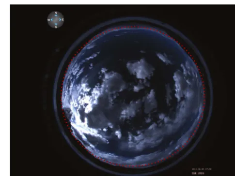
and is enclosed by a weather protection box. The TCI is pro-grammed to acquire images at fixed intervals, and all im-ages are stored in color JPEG format with a resolution of 1392×1040 pixels. Note that these images are rectangular in shape but the mapped whole sky is circular, in which the cen-ter is the zenith and the horizon is along the border. Figure 2 displays an example of such an all-sky image. Because the region near the circular border contains certain terrestrial ob-jects, such as trees and buildings on the horizon of the TCI,
Figure 2. An all-sky image example used in this work (3
Octo-ber 2012, 17:30 GMT+8). The area marked by the red circle refers
to the circle of interest.
we eliminate the area out of circle of interest (COI). COI is defined by the center(cx, cy)and radiusr. We set (cx, cy)
with(718,536)andrwith 442 in this work. Note that COI is the exact area for feature extraction and type identification.
We screened the complete image set that was observed during August 2012 to July 2014 and selected 5000 all-sky images in this work according to our predefined cloud classes (see next section). We did our best to ensure that the data set includes a large variety of different cloud forms. The data set 1contains 1000 independent images per cloud class. 2.2 Cloud classes
Traditionally, manual cloud classification takes cloud shape as a basic factor, together with shape development and in-terior micro-structure of the cloud. Clouds are divided into 29 varieties of 10 genera in 3 families with high, mid-, and low levels, according to the “Linnean” system developed by Howard (1803). These criteria are used by surface observers, but they are unsuitable for automatic cloud classification. Calbo and Sabburg (2008) defined eight different sky con-ditions for automatic cloud classification, while Heinle et al. (2010) considered seven types. Note that there are also other configurations of cloud types for automatic cloud classifica-tion, and recent reviews can be found in Tapakis and Char-alambides (2013).
Stratiform, cumuliform, and cirriform clouds are the most common sky conditions, and they are primary classes in many cloud classification systems (Tapakis and Charalam-bides, 2013; Xia et al., 2015). Furthermore, a sky condition obtained by an all-sky imager often contains multiple types of clouds (Cheng and Yu, 2015). We, therefore, define five
1The data set is available at http://icn.bjtu.edu.cn/visint/
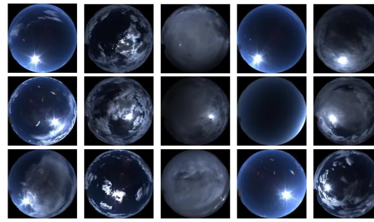
(a) Cirriform (b) Cumuliform (c) Stratiform (d) Clear sky (e) Mixed cloudiness
Figure 3. Classic all-sky images of the five sky condition classes.
Table 1. Sky condition classes proposed in this work.
Sky condition classes Description Cloud types
Cirriform Thin clouds that are wispy and feathery-like Ci, Cc and Cs
Cumuliform Thick clouds that are puffy and cotton-like Cu, Cb and Ac
Stratiform Layered clouds that stretch out across the sky St, As, Sc and Ns
Clear sky Clear sky without cloud No clouds
Mixed cloudiness Mixed sky conditions with more than one cloud type
that covers the sky more than 20 %
Co-occurrence
sky conditions for cloud classification as demonstrated in Ta-ble 1. In our data set, most images of Cc and Cs are bright and light blue, because the aerosol optical depth is small in Tibet (29.25◦N, 88.88◦E) where the data set was collected. These features are very similar to those of Ci as shown in Fig. 3a. In addition, Cc, Cs, and Ci all belong to high-level clouds. So we sort these cloud types into the same category. Cumuli-form clouds are usually puffy in appearance, similar to large cotton balls; while stratiform clouds are horizontal and lay-ered clouds that stretch out across the sky like a blanket. An image of these classes contains a single cloud type, but an image of mixed condition contains more than one cloud type together. Figure 3 displays some typical all-sky images of these five sky conditions. This configuration of cloud classes is similar to those used by Liu et al. (2011) and Xia et al. (2015), except for the augmented class of mixed cloudiness, which is never investigated in the literature but often occurs in all-sky images.
3 Cloud classification based on a bag of micro-structures
In this section, we first introduce the background of BoMS and the pipeline of the cloud classification method. Then we describe the details of BoMS, including patch descriptor, dictionary of micro-structures, and holistic image represen-tation. At last, the classifier with SVM is presented.
3.1 Overview of the proposed cloud classification method
3.1.1 Review of the bag-of-words model
reject very common words (such as “the”, “a” and “does”), because they occur in most documents and are not meaning-ful enough to discriminate different documents. After that, the remaining words are assigned with a unique label, and the document is represented by a vector that indicates the oc-currences of these words. Note that each component of the vector is often weighted in various ways in order to improve its degree of discrimination (Baeza-Yates and Ribeiro-Neto, 1999). Finally, such vectors are used as features for docu-ment classification or used to build an index for information retrieval.
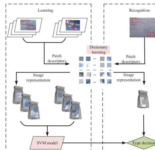
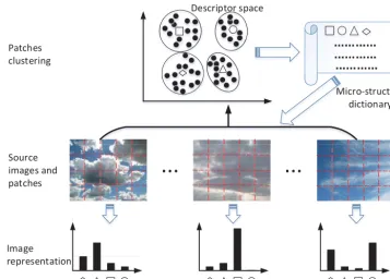
3.1.2 Pipeline of the cloud classification method Inspired by the bag-of-words model, we propose the new cloud classification method, which treats a cloud image as a collection of micro-structures. More specifically, the pro-posed method includes two aspects: learning and recogni-tion (as shown in Fig. 4). The learning procedure is offline and carries out two tasks: learning the dictionary of micro-structures and training the SVM model. Recognition proce-dure analyzes an input image and identifies its cloud class. It includes four main procedures.
1. It divides an input image into patches (maybe with over-lap) and extracts a description for each patch accord-ing to its appearance. In other words, the input image is treated as a collection of patches, rather than raw pixels. 2. It assigns patch descriptors to a set of predetermined micro-structures by vector quantization. Each patch is mapped to a label of certain micro-structure in a learned dictionary, so the input RGB image can be transformed into a label matrix. Each element of the label matrix refers to an index of a micro-structure. Accordingly, the image is regarded as a bag of micro-structures, just as a document is represented by its words.
3. It constructs a holistic image representation based on BoMS. The histogram of micro-structures is calculated and used as the feature vector of the input image. 4. It applies a SVM classifier to identify the cloud type of
the input image, which is represented by a histogram of micro-structures.
We refer to the quantized patch descriptors as micro-structures, because each micro-structure represents a com-mon pattern or appearance shared by many patches. Micro-structures for a cloud image play the same role as words for a text document, though they do not necessarily have an ac-tual meaning as “wispy cloud”, or “puffy cloud”.
SVM model Type decision
Dictionary learning
Learning Recognition
Image representation Patch
descriptors descriptorsPatch
Image representation
Ċ Ċ Ċ Ċ Ċ Ċ Ċ
Ċ Ċ
Figure 4. The pipeline of the cloud classification method based on BoMS.
3.2 Cloud representation of BoMS
3.2.1 Patch descriptor based on appearance
A cloud image is regarded as a collection of local patches, rather than simple pixels. Image patches should be firstly de-scribed by certain feature vectors (named descriptors) based on their visual appearance. Of course, this descriptor should be discriminative for cloud patches. We apply statistical mea-surements of color and contrast to describe image patches, because color and contrast are the most important appearance features to distinguish cloud patches from others patterns.
Firstly, a cloud image is equally divided into several patches (maybe with overlap). Given an imageI with width wand heighth, a patch refers to a square area defined by the top-left point (px, py) and size s, 1≤s≤min(w, h).
Fur-thermore, all patches are indirectly specified by the sampling step τ. Of course, if τ equals s, a cloud image would be segmented into grids without overlap. Note that the border patches that are partly beyond the scope of COI are discarded because they contain nonsense pixels.
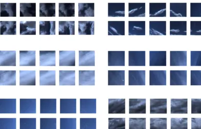
Figure 5. Samples of image patches randomly selected from certain clusters. All images in a cluster are assigned with an identical label of micro-structure.
so improved contrast features based on such difference are included in the patch descriptor as well. More specifically, the patch descriptor is calculated as follows.
Mean, standard deviation, and skewness of blue component
Color is one of the most important characteristics to distin-guish clouds from sky. Especially, the blue component has the highest discrimination power. So the meanMb, standard deviationDband skewnessSbof blue components are used in the patch descriptor.Mbencodes the main color appear-ance, whileDbandSbpartly describe the texture character-istics of an image patch.
Mb=
Xs2 i=1Bi/s
2, (1)
Db=
r Xs2
i=1(Bi−Mb)
2/ s2−1
, (2)
Sb= 1 s2−1
Xs2 i=1
B
i−Mb
Db
3
, (3)
whereBi refers to the intensity value of blue channel for the
pixeliin a patch with sizes.
Mean, standard, and skewness of the ratio of red and blue components
The ratio of red and blue components is a popular feature used to classify cloud from sky, because a clear sky scatters
more blue than red light and appears blue, whereas clouds scatter blue and red light with similar extent and appear white or gray (Calbo and Sabburg, 2008). So the meanMt, standard
deviationDt, and skewnessStof the ratio values are adopted
as supplements for the above measurements of blue compo-nent.
Mt= Xs2
i=1Rti/s
2, (4)
Dt= r
Xs2
i=1(Rti−Mt)
2/ s2−1
, (5)
St=
1 s2−1
Xs2 i=1
Rt
i−Mt
Dt 3
, (6)
whereRti(=Ri/Bi)represents the ratio of red component
and blue component.
Contrast between color components
ĊĊĊĊ ĊĊĊĊ ĊĊĊĊ
...
...
Source images and patches Patches clustering
Descriptor space
Micro-structure dictionary
Image representation
... ...
...
M
M
M
M
Figure 6. Image representation based on micro-structures, in which patch descriptors are grouped to construct micro-structure dictionary, and histogram of such micro-structures in an image is used as its representation.
components. C1=
Mr−Mg Mr+Mg
, (7)
C2=
Mr−Mb Mr+Mb
, (8)
C3=
Mg−Mb Mg+Mb
, (9)
whereMr,Mg, andMbrefer to the mean values of red, green, and blue components in the image patch, respectively.
Consequently, each patch can be represented by a nine-dimensional feature vector:
D=< Mb, Db, Sb, Mt, Dt, St, C1, C2, C3> . (10) A sampled collection of such descriptors are used to con-struct a micro-con-structure dictionary (see the following sec-tion). Note that each dimension ofDis normalized to[0,1], in order to eliminate the effect of magnitude.
3.2.2 Learning dictionary of micro-structures with kmeans algorithm
Dictionary of micro-structures is one of the most important aspects of BoMS, and it is learned offline by the k means algorithm (Han et al., 2006). First, a large number of im-age patches are equally sampled from the data set, and their descriptors are extracted to form a collection. Second, the descriptor collection is clustered bykmeans algorithm and
divided intokclusters. Finally, the centroids of these clusters are regarded as structures, and they form the micro-structure dictionary. A micro-micro-structure represents a specific local pattern shared by all patches assigned to it. Figure 5 shows examples of image patches belonging to particular clusters.
K-means clustering is a method of vector quantization, which is popular for cluster analysis in data mining. Given a set of patch descriptors {D1, D2,· · ·, Dn}, k means
al-gorithm groups the n descriptors into k(≤n) sets S= {S1, S2,· · ·, Sk}by minimizing the sum of squared Euclidean
distances between descriptors and their corresponding cen-troids. The objective function ofk means is formulated as follows:
arg
S
min
k X
i=1
X
D∈Si
kD−µik2, (11)
whereµirepresents the centroid of clusteri. Given an initial
set ofkcentroids{µ01, µ20,· · ·, µ0k},kmeans algorithm alter-nates between assignment step and update step.
– Assignment step. It assigns each descriptor to its nearest cluster centroid and obtains grouped clusters as follows:
Sit =
Dp Dp−µti
2 ≤
Dp−µ
t j
2
,∀j,1≤j≤k
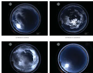
(a) Mixture to cirriform (b) Mixture to cumuliform
(c) Mixture to stratiform (d) Cirriform to clear sky
Figure 7. Some misclassified all-sky images.
– Update step. It recalculates the centroids of new clus-ters. A new centroid is updated as follows:
µti+1=1
Sit
X
Dj∈Sit Dj.
The algorithm is regarded as converged when the assign-ments no longer change or the number of iteration has reached a predefined value. After the algorithm is con-verged, the dictionary is constructed and denoted as V = {µ1, µ2,· · ·, µk}, whereµi refers to the prototype of
micro-structure with labelsi. The number of clusterskdetermines
the size of the dictionary, which can vary from hundreds to thousands.
3.2.3 Image representation based on BoMS
Image representation refers to the characteristics of an all-sky image and is encoded by a numeric feature vector. Image representation is different from the patch descriptor, but it is built on patch descriptors as shown in Fig. 6. Inspired by the bag-of-words model, we bring forward the “bag of micro-structure” model to extract the image representation.
Firstly, an all-sky image is divided into several patches (see Sect. 3.2.1), and each patch maps to certain type of micro-structure in the dictionary. Assume that the image is
divided intompatches denoted as{D1, D2,· · ·, Dm}.Di(1≤
i≤m) is a nine-dimensional vector and is mapped to cer-tain micro-structure label si(∈ [1, k])by searching for the
nearest micro-structure among the dictionaryV. Thereby, the descriptor set{D1, D2,· · ·, Dm}is transformed into a label
set{L1, L2,· · ·, Lm}, whose value of each element refers to
the index of a certain micro-structure. The label set is com-posed of many micro-structures, just as a document consists of words.
After that, we transform the image, which is denoted as a label set, into a representation suitable for the learning al-gorithm. We apply an attribute-value representation for all-sky images. Basically, each distinct micro-structuresi
corre-sponds to a feature, assigned with the valuetithat counts the
number of occurrences of micro-structuresi. In order to
high-light some important micro-structures, we apply a weighting strategy and represent the image by a vector:
F = ht1, t2,· · ·, tki. (12)
ti(1≤i≤k) refers to the weighted frequency of
micro-structuresiand is calculated by
ti=nilog
N Ni
, (13)
whereni is the number of occurrences of micro-structure
si, and N is the number of images in the whole data set.
In essence, TF (term frequency) and IDF (inverse document frequency) are two major factors in the weighting strategy (Baeza-Yates and Ribeiro-Neto, 1999). TF weights micro-structures more highly if they occur more often in an image, while IDF decreases the weights of the micro-structures that appear often in the data set because these micro-structures do not help to discriminate between different images.
This representation is analogous to the bag-of-words model for a document in terms of form and semantics. Micro-structures reveal characteristics of local patterns for all-sky cloud images, just as words convey meanings of a document. Note that both representations are sparse and high dimen-sional.
3.3 Classifier with SVM
Support vector machines are based on the structural risk minimization principle from computational learning theory (Vapnik, 2000). Basically, the SVM classifier learns a hy-perplane that separates two-class data with maximal margin. The margin is defined as the distance of the closest training sample to the separating hyperplane. Given a training set X and corresponding class labels Y that takes value±1, SVM finds a decision function:
f (x)=sign(wTx+b),
wherewandbrefer to the parameters of the hyperplane. The SVM applies two strategies to address the data set that is not linearly separable. Firstly, it introduces a regularization term that penalizes misclassification of samples in proportion to their distance from the hyperplane, and this regularization term is weighted by the parameterC. Secondly, a mapping8 is considered to transform the original data space of X into another feature space. The feature space may have a high or even infinite dimension. Because SVM can be formulated by the terms of scalar products in the mapped feature space, it is avoidable to directly define such mapping by introducing the kernel function K(u, v)=8(u)T×8(v). In the kernel formulation, the decision function can be written as
f (x)=sign(yiαiK(x, xi)+b), (14)
wherexi is a feature vector from the training set X andyi
is the label of xi. The parameters αi are learned by SVM,
and they are typically zero for mosti. The feature vectorsxi
corresponding to nonzeroαi are known as support vectors.
In the cloud classification method, the input features re-fer to the BoMS representation in Eq. (12). We take the one-against-all approach for the multi-class problem. That is, there are five classes for all-sky images, so we train five SVM classifiers. Classifier model idistinguishes images between categoryiand all the other four categories. Given a test im-age, we assign it to the class with the largest SVM output.
There are two reasons motivating us to select SVM rather than other methods, such as KNN and artificial neural
net-works. On the one hand, the image representation based on BoMS is high dimensional (more than 100 dimensions in our experiments). SVM has the potential to handle large fea-ture space because it embraces overfitting protection, and it is more efficient for space and time compared to KNN. On the other hand, the image representation of BoMS is sparse. In other words, the feature vector contains only few entries that are not zero. SVM is proven to be well suited for prob-lems with dense concepts and sparse instances (Melgani and Bruzzone, 2004; Tong and Koller, 2002).
4 Results and discussion
In this section we evaluate the performance of BoMS, com-pared with the baseline (Heinle et al., 2010), and investigate the effect of the key parameters in BoMS.
We apply 10-fold cross-validation to estimate the perfor-mance of classification methods. The data set is randomly partitioned into 10 equal sized subsets. One single subset is retained for validation, and the remaining nine subsets are used as training data. The cross-validation process is then repeated 10 times. During the cross-validation, each subset is used exactly once as validation; meanwhile, each image in the data set is also used for validation exactly once. Fi-nally, the measure of performance is defined by accuracy (Ac), which is given by
Ac=Correctly classified image number
Total image number . (15)
We conduct each experiment three times and take average values as final results.
4.1 Performance of BoMS
Table 2 demonstrates the confusion matrix of BoMS method, in which the patch sizes equals 12 with a stepτ =6 and the dictionary sizekequals 500. The kernel of SVM selects linear kernel function, and the regularizationCis set to 62.5, which is optimized by a search strategy.
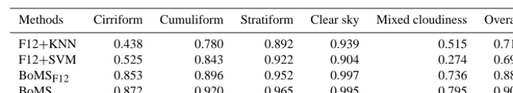
Table 3. Comparison of BoMS and baselines according to accuracy of each class.
Methods Cirriform Cumuliform Stratiform Clear sky Mixed cloudiness Overall
F12+KNN 0.438 0.780 0.892 0.939 0.515 0.713
F12+SVM 0.525 0.843 0.922 0.904 0.274 0.694
BoMSF12 0.853 0.896 0.952 0.997 0.736 0.887
BoMS 0.872 0.920 0.965 0.995 0.795 0.909
4.2 Performance comparisons with the baselines In order to verify the advantage of BoMS, we compare its classification performance with the following three methods: – F12+kNN is the original method proposed by Heinle et al. (2010), and it acts as the baseline in this com-parison. We set k with 9 by an optimized search procedure and set the weight vector of features with [1,1,1,1,1,1,2,1,2,2,3,1], which is suggested by Heinle et al. (2010).
– F12+SVM method applies the 12-dimensional features used in (Heinle et al., 2010) but replaces kNN with SVM, in order to investigate the influence of classifier. The kernel of SVM selects linear kernel as well. – BoMSF12 method applies the framework of BoMS,
but its patch descriptor is replaced by Heinle’s 12-dimensional features, rather than 9-12-dimensional fea-tures described in Sect. 3.
Table 3 presents the comparison results. BoMS outper-forms all other methods. Especially, BoMS outperoutper-forms F12+KNN with regards to all five classes and achieves an increase of 19 % overall accuracy. There are two main differ-ences between BoMS and F12+KNN: feature representation and classifier model. What makes sense for such improve-ment? We first compare F12+KNN and F12+SVM and ob-serve that F12+SVM does not make an improvement. This result indicates that SVM does not lead to better performance just based on traditional features. The comparison between F12+SVM and BoMSF12 shows that BoMSF12 is notably better than F12+SVM. So it can be deduced that the image representation based on BoMS contributes to the excellent performance.
Figure 8. The curve of overall accuracy of BoMS with different patch sizes.
4.3 Parameter analysis
In the framework of BoMS, patches are the fundamental ob-jects, and they are mainly determined by patch sizes. What is the influence of parameters?
Figure 8 displays the accuracy curve of BoMS according to differents. Note that the sampling stepτ is set to s/2 in this experiment. Generally, the accuracy for most values of patch sizesis greater than 86 %, and smaller patch size can result in better accuracy. Especially, we get the best perfor-mance settingswith 12. This result reveals that structure in-formation of image patches is significant for cloud classifi-cation, but patches with too small size maybe do not encode enough structure information. Meanwhile, large patches have too large variations to construct efficient micro-structures.
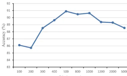
Figure 9. The curve of overall accuracy of BoMS with different dictionary sizes.
experiment results show that classification accuracy is robust forτ, and it is the best choice to setτ withs/2, regarding the accuracy and computational complexity.
The dictionary of micro-structures is another core factor for BoMS, and its sizeknot only determines the dimension of the image representation but also influences the classi-fication performance. Figure 9 displays the accuracy curve of BoMS according to different dictionary sizek. Generally, BoMS achieves stable performance with an accuracy greater than 88 %, when dictionary size kis more than 300. Espe-cially, BoMS obtains the best performance withk=500. We can account for this result with two aspects. Firstly, a small dictionary of micro-structures just contains limited distinct patterns, since one micro-structure represents one common pattern that is shared by many image patches. As a result, the BoMS with small dictionary is not discriminative enough for cloud classification. Secondly, the dictionary would be sat-urated with micro-structures when its size is large enough, and a proper micro-structure would be divided into multi-ple sub-patterns if the dictionary size further increased. How-ever, such sub-patterns cannot promote classification perfor-mance.
Moreover, the dimension of BoMS equals with sizek. In other words, larger dictionary size results in a higher dimen-sion of cloud representation. Consequently, a medium dic-tionary size is a good choice, considering the computational complexity.
5 Conclusions
This study presents the new cloud classification method based on a bag of micro-structures, whereas most state-of-the-art methods (Heinle et al., 2010; Liu and Zhang, 2015; Kliangsuwan and Heednacram, 2015; Cheng and Yu, 2015) apply traditional features based on pixels. In this method, an all-sky image is treated as a collection of micro-structures just as a document consists of words, and it is represented by a high-dimensional histogram of micro-structures. Sub-sequently, the SVM classifier is used to identify the cloud
type of the all-sky image. A large data set is constructed with actual all-sky images captured by the TCI located in Tibet (29.25◦N, 88.88◦E), and evaluation is carried out to verify
the performance of BoMS. The experiment results demon-strate that BoMS achieves a high accuracy of 90.9 %, and it outperforms the state-of-the-art method proposed by Heinle et al. (2010). Moreover, the experiments on the influence of key parameters, including patch sizesand dictionary sizek, are carried out to verify the robustness of BoMS.
We will extend our research in future from the follow-ing aspects. Firstly, we will extensively investigate differ-ent patch descriptors and find out more efficidiffer-ent patch rep-resentation for BoMS. Secondly, we are going to study topic models for cloud images in order to reduce the dimension of cloud representation and further improve classification ac-curacy. Lastly, we will conduct research to establish a con-figuration of sky conditions, which is suitable for automatic cloud classification systems.
Acknowledgements. This work is partly supported by the National
Key Scientific Instrument and Equipment Development Projects of China (2012YQ11020504), Fundamental Research Funds for the Central Universities (2014JBZ003), the National Natural Science Foundation of China (41105121), and the Basic Research Fund of Chinese Academy of Meteorological Sciences.
Edited by: C. von Savigny
References
Ameur, Z., Ameur, S., Adane, A., Sauvageot, H., and Bara, K.: Cloud classification using the textural features of Meteosat im-ages, Int. J. Remote Sens., 25, 4491–4503, 2004.
Baeza-Yates,R. and Ribeiro-Neto, B.: Modern Information Re-trieval, ACM Press, Addison Wesley, USA, 82 pp., 1999. Calbo, J. and Sabburg, J.: Feature extraction from whole-sky
ground-based images for cloud-type recognition, J. Atmos. Ocean. Techn., 25, 3–14, 2008.
Cheng, H.-Y. and Yu, C.-C.: Block-based cloud classification with statistical features and distribution of local texture features, At-mos. Meas. Tech., 8, 1173–1182, doi:10.5194/amt-8-1173-2015, 2015.
Han, J., Kamber, M., and Pei, J.: Data Mining: Concepts and Tech-niques, Morgan Kaufmann, San Francisco, CA, USA, 401 pp., 2006.
Heinle, A., Macke, A., and Srivastav, A.: Automatic cloud classi-fication of whole sky images, Atmos. Meas. Tech., 3, 557–567, doi:10.5194/amt-3-557-2010, 2010.
Howard, L.: On the Modifications of Clouds, 3rd edn., J. Taylor, London, UK, 28 pp., 1803.
Hu, X., Wang, Y., and Shan, J.: Automatic recognition of cloud im-ages by using visual saliency features, IEEE Geosci. Remote S., 12, 1760–1764, doi:10.1109/LGRS.2015.2424531, 2015. Huang, Y., Wu, Z., Wang, L., and Tan, T.: Feature coding in image
Economou, G.: Cloud detection and classification with the use of whole-sky ground-based images, Atmos. Res., 113, 80–88, 2012. Kliangsuwan, T. and Heednacram, A.: Feature extraction tech-niques for ground-based cloud type classification, Expert Syst. Appl., 42, 8294–8303, doi:10.1016/j.eswa.2015.05.016, 2015. Li, Q., Lu, W., and Yang, J.: A hybrid thresholding algorithm for
cloud detection on ground-based color images, J. Atmos. Ocean. Techn., 28, 1286–1296, 2011.
Li, Q., Lu, W., Yang, J., and Wang, J. Z.: Thin cloud detection of all-sky images using Markov random fields, IEEE Geosci. Remote S., 9, 417–421, 2012.
Liu, L., Sun, X. J., Chen, F., Zhao, S. J., and Gao, T. C.: Cloud classification based on structure features of infrared images, J. Atmos. Ocean. Techn., 28, 410–417, 2011.
Liu, S. and Zhang, Z.: Learning discriminative salient LBP for cloud classification in wireless sensor networks, Int. J. Distrib. Sens. N., 501, 327290, 1–7, 2015.
Liu, S., Wang, C., Xiao, B., Zhang, Z., and Shao, Y.: Salient local binary pattern for ground-based cloud classification, Acta Mete-orol. Sin., 27, 211–220, 2013.
Long, C. N., Sabburg, J. M., Calbó, J., and Pagès, D.: Retrieving cloud characteristics from ground-based daytime color all-sky images, J. Atmos. Ocean. Techn., 23, 633–652, 2006.
Mantelli Neto, S. L., von Wangenheim, A., Pereira, E. B., and Co-munello, E.: The use of Euclidean geometric distance on RGB color space for the classification of sky and cloud patterns, J. At-mos. Ocean. Techn., 27, 1504–1517, 2010.
Melgani, F. and Bruzzone, L.: Classification of hyperspectral re-mote sensing images with support vector machines, IEEE T. Geosci. Remote, 42, 1778–1790, 2004.
Ricciardelli, E., Romano, F., and Cuomo, V.: Physical and sta-tistical approaches for cloud identification using Meteosat Sec-ond Generation-Spinning Enhanced Visible and Infrared Imager Data, Remote Sens. Environ., 112, 2741–2760, 2008.
Geosci. Remote, 49, 5008–5015, 2011.
Tapakis, R. and Charalambides, A.: Equipment and methodologies for cloud detection and classification: a review, Sol. Energy, 95, 392–430, 2013.
Tong, S. and Koller, D.: Support vector machine active learning with applications to text classification, J. Mach. Learn. Res., 2, 45–66, 2002.
Urquhart, B., Kurtz, B., Dahlin, E., Ghonima, M., Shields, J. E., and Kleissl, J.: Development of a sky imaging system for short-term solar power forecasting, Atmos. Meas. Tech., 8, 875–890, doi:10.5194/amt-8-875-2015, 2015.
Vapnik, V.: The Nature of Statistical Learning Theory, Springer Sci-ence and Business Media, New York, USA, 123 pp., 2000. Xia, M., Lu, W., Yang, J., Ma, Y., Yao, W., and Zheng,
Z.: A hybrid method based on extreme learning machine and k-nearest neighbor for cloud classification of ground-based visible cloud image, Neurocomputing, 160, 238–249, doi:10.1016/j.neucom.2015.02.022, 2015.
Yang, J., Lu, W., Ma, Y., and Yao, W.: An automated cirrus cloud de-tection method for a ground-based cloud image, J. Atmos. Ocean. Techn., 29, 527–537, doi:10.1175/JTECH-D-11-00002.1, 2012. Yang, J., Min, Q., Lu, W., Yao, W., Ma, Y., Du, J., Lu, T., and
Liu, G.: An automated cloud detection method based on the green channel of total-sky visible images, Atmos. Meas. Tech., 8, 4671–4679, doi:10.5194/amt-8-4671-2015, 2015.