Ocean Sci., 10, 411–426, 2014 www.ocean-sci.net/10/411/2014/ doi:10.5194/os-10-411-2014
© Author(s) 2014. CC Attribution 3.0 License.
On the tides and resonances of Hudson Bay and Hudson Strait
D. J. Webb
National Oceanography Centre, Southampton SO14 3ZH, UK Correspondence to: D. J. Webb ([email protected])
Received: 30 September 2013 – Published in Ocean Sci. Discuss.: 5 November 2013 Revised: 3 April 2014 – Accepted: 3 April 2014 – Published: 28 May 2014
Abstract. The resonances of Hudson Bay, Foxe Basin and Hudson Strait are investigated using a linear shallow water numerical model. The region is of particular interest because it is the most important region of the world ocean for dissi-pating tidal energy.
The model shows that the semi-diurnal tides of the re-gion are dominated by four nearby overlapping resonances. It shows that these not only affect Ungava Bay, a region of extreme tidal range, but they also extend far into Foxe Basin and Hudson Bay and appear to be affected by the geometry of those regions. The results also indicate that it is the four resonances acting together which make the region such an important area for dissipating tidal energy.
1 Introduction
In his study of tidal dissipation on the world ocean, Miller (1966) estimated that Hudson Bay and the Labrador Sea dis-sipated 140 GW of M2 tidal energy. This made it the fifth most important region of tidal dissipation, the first four being the Bering Sea, the Sea of Okhotsk, the Northwest Australian Shelf and the European Shelf.
More recent studies have completely changed this picture. Le Provost and Rougier (1997), using a numerical model, found that the M2 tide dissipated 313 GW in the Hudson Bay region. This made it their most important region for tidal dis-sipation.
Egbert and Ray (2001) assimilated satellite altimeter data into an ocean model and again found the Hudson Bay region to be the most important, the M2 tide dissipat-ing 261 GW. Next in importance was the European Shelf (∼208 GW), followed by the Northwest Australian Shelf (∼158 GW), the Yellow Sea (∼149 GW) and the Patagonian Shelf (∼112 GW).
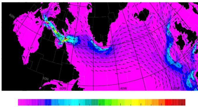
The importance of the Hudson Bay complex is also em-phasised if one plots the M2 energy flux vectors for the North Atlantic. This has been done in Fig. 1, making use of the satellite-derived tidal fields of Egbert and Erofeeva (2002). In the eastern North Atlantic the figure shows a northward flux of tidal energy associated with a propagating Kelvin wave. Part of the energy is lost to the European Shelf but a large amount continues north. It then turns westwards and passes south of Greenland before converging on Hudson Strait.
If the fluxes of Fig. 1 are integrated along lines between 44◦W, 42◦N and the coasts of Spain and Greenland, the results show that the M2 tide fluxes 490 GW northwards into the northeast Atlantic and that 220 GW passes south of Greenland towards Hudson Strait. At the entrance to Hudson Strait the flux of energy is 250 GW – the increase being due to a small northward flow of tidal energy on the western side of the Atlantic.
Thus not only is the Hudson Bay complex the major tidal dissipation region of the global ocean, it is also so effective that no energy-transporting Kelvin wave continues south-wards along the coast of Labrador and Newfoundland. This is in marked contrast to the behaviour on the eastern side of the ocean where a large fraction of the energy flux continues past the resonant European continental shelves. Even though the entrance to Hudson Strait is only 70 km wide, it transmits much more energy than the Celtic Sea, at the entrance to the English Channel and Irish Sea, which is over 400 km wide.
Continental shelf regions with large amounts of tidal dis-sipation are usually associated with resonances of the shelf. Examples are the Bristol Channel (Fong and Heaps, 1978; Webb, 2013a), the Patagonian Shelf (Huthnance, 1980) and the Northwest Australian Shelf. Such regions are usually as-sociated with high tides, so one possible reason why Hud-son Bay was overlooked is that it is only recently that Leaf
40
0 80 120 160 200 240 280 320
50N
60N
40W
60W 20W
Figure 1. Energy flux vectors for the M2 tide in the north Atlantic, based on from data from OTIS2 (Egbert and Erofeeva, 2002). Energy
flux in units of MW m−1.
Bay, part of Ungava Bay1near the entrance to Hudson Strait, has been reported as having the world’s second highest tidal range (O’Reilly et al., 2005).
The high tides of Ungava Bay were studied by Arbic et al. (2007) using a time-dependent numerical model. This showed that the tides of the region were affected by a quarter-wavelength resonance between the coast and the deep ocean. The resonance mode also showed maxima elsewhere in Foxe Basin and Hudson Bay which, following the recent study of the English Channel and Irish Sea (Webb, 2013a), might indi-cate the presence of additional resonances affecting the tides. The English Channel and Irish Sea study used a time-independent model. This has the advantage that it can be run for complex values of angular velocity and so allows a de-tailed study of the resonant structure of a region.
The study uses a method of analysis in regular use by physicists (e.g. Morse and Feshbach, 1953; Mathews and Walker, 1965; Courant and Hilbert, 2008; Riley et al., 1998) but not widely used by physical oceanographers. In this, the response to forcing of a linear (or approximately linear) sys-tem is shown to depend on the resonance properties of the system. Use is also made of the fact that, for such systems, the response to periodic forcing is described by an analytic function, the response function, whose poles correspond to the resonant angular velocities or eigenvalues of the sys-tem. Once the resonance eigenvalues and eigenfunctions are known, the response of the system to any kind of forcing can be calculated.
Although the tides are affected by nonlinearities, the am-plitude of the nonlinear tidal constituents are small over most of the ocean. As a result, the assumption of linearity is a good
1Leaf Bay is adjacent to Hopes Advanced Bay, indicated by the
letter U in Fig. 2. Other locations discussed in the text are also shown in this figure.
first approximation for any study of the large-scale behaviour of the tides.
If the system is frictionless, the poles of the response func-tion lie on the real angular velocity axis and the eigenfunc-tions corresponding to the different resonances are orthogo-nal. If friction is present, as it is within the ocean, the poles lie off the real axis and the imaginary component of angular velocity then equals the inverse decay time of the resonance. With friction the eigenfunctions are also not orthogonal. This complicates the analysis, but it is still tractable making use of the adjoint set of equations and eigenvalues.
A simple example of the approach, using a 1-D tidal model, is given in Webb (2011). Further details and exam-ples, solving Laplace’s tidal equations in more realistic re-gions of ocean, are given in other papers from the present se-ries (Webb, 2012, 2013a, b, 2014). Results from three much earlier papers on the tides (Webb, 1973, 1976, 1982) are also relevant.
In the present paper, a model similar to that used for the English Channel study is used to study the Hudson Bay re-gion. The study aims to investigate the resonances and also the impact of three unusual properties of the region.
The first of these concerns Hudson Strait. With central depths of over 300 m, the strait is much deeper than is nor-mal for continental shelf regions. The extra depth means that tidal wavelengths are longer than normal and frictional ef-fects are smaller. As a result there is a potential for quarter and three-quarter wavelength resonances extending far into Hudson Bay in the south and into Foxe Basin in the north.
D. J. Webb: Tidal resonances of Hudson Strait 413
Finally, the open region of Hudson Bay in the south is large enough to support a circulating wave. This may act like a resonator but a damped circulating wave might also have the properties of a damped infinite channel.
Section 2 of the paper gives the details of the model used for the study. Section 3 then reports on the results obtained using real values of angular velocity and Sect. 4 extends this to complex values of angular velocity. Section 5 is concerned with the main resonances affecting the semi-diurnal tides and Sect. 6 investigates how these combine to generate the ob-served response within the tidal band. Finally the discussion section reviews the main results of this study and considers their implications.
2 The numerical model
The model used to study the Hudson Bay, Hudson Strait and Foxe Basin region is based on that described by Webb (2013a). It solves the linear form of Laplace’s tidal equations at a single angular velocity using finite difference equations based on an Arakawa C-grid distribution of model variables. The model covers the region bounded by the latitude and longitude lines at 94.25◦W, 57.5◦W, 51.125◦N and 70.375◦N, with a resolution of 0.125◦ in the east–west di-rection and 0.25◦in the north–south direction. The other free parameters are the linear coefficient of bottom friction and the minimum cell depth. These were set to 0.2 cm s−1 and 2.5 m, as in Webb (2013a).2
Coastlines and cell depths are based on the GEBCO coast-line depth data sets (IOC et al., 2003). The GEBCO depth data is at a higher resolution (1/60◦) than that used for the model grid, so depths were calculated such that the volume of each model grid cell is the same as the corresponding GEBCO region. Away from coastlines this is equivalent to them having the same average depth.
As discussed in Webb (2013a), coastlines are specified to pass through velocity points, such that the normal velocity at the coast can be specified to be zero. Open boundaries are specified to follow lines of sea surface height points.
In the extreme northwest, the model closes off the narrow Fury and Hecla Strait which connects Foxe Basin with the Gulf of Boothia. The east of the strait is blocked by Elder and Ormonde islands, with the largest of the narrows being only 2 km wide. The total cross-section is so small that little tidal energy can flow into or out of Foxe Basin via this route. The open boundary includes part of the Labrador Sea with depths extending down to 3000 m. In this region of the model the northern and southern limits are at 57.125◦N and
2The model allows the linear coefficient of bottom friction to be
a function of position. As discussed by Hunter (1975) this allows the mean effect of a realistic non-linear bottom friction term to be in-cluded. However, this requires additional runs of a fully non-linear model and has not be used for the study reported here.
55 60 65 70
90 80 70 60
Longitude (W)
Latitude
C
W U
R2FB R3 R4
R1 R
S H
Foxe Basin
Hudson Bay
James Bay
CS
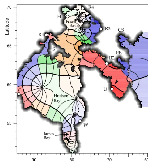
Figure 2. Model solution for the M2 tide. Thick lines are contours
of amplitude at 0.5 m, 1 m, 2 m and 3 m. Thin lines are contours of phase, at intervals of 30 degrees, relative to the equilibrium tide at
Greenwich. Colours denote phase quadrant (red, 0◦–90◦; orange,
90◦–180◦; green, 180◦–290◦; blue, 270◦–360◦) with the more
in-tense colours denoting higher amplitudes. The tide gauge stations are C, Churchill; H, Hall Beach; R, Repulse Bay; W, Great Whale River; U, Hopes Advance Bay (Ungava Bay). Locations R1 to R4, S (Southampton Island), FB (Frobisher Bay) and CS (Cumberland Sound) are referred to elsewhere in the paper.
66.875◦N. As a result the open boundary in the east includes almost all of the energy inflow region shown in Fig. 1.
For the open boundary, Webb (2013a) used Dirichlet boundary conditions in which the tidal height on the bound-ary is fixed by observations. The tangential velocity is set to the value one row in from the open boundary.
The present version of the model uses the same open boundary condition for the validation stage where the deep ocean tide is known. Then in the remainder of the study it is changed to allow radiation of energy back into the deep ocean. The radiation scheme is based on that of Flather (1976) which is often used for time-dependent models. De-tails are given in Appendix B1.
3 The M2 tide
The model was validated using a simulation of the M2 tide. For this the model was forced at the open boundary with tidal amplitudes and phases taken from a global assimilation of satellite altimeter data (Egbert and Erofeeva, 2002). The
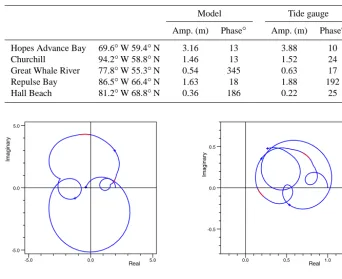
model result is shown in Fig. 2 and the values at representa-tive stations compared with tidal observations (IHB, 1954) in Table 1.
The agreement is good at Hopes Advance Bay, in the west of Ungava Bay near Leaf Basin. The phase in the deep ocean is around 300◦so the coast here is approximately 70◦out of phase. Given that some of the highest tides in the world are found in Leaf Basin, this phase difference between the coast and the deep ocean is less than the 90◦expected from a pure quarter-wavelength resonance.
Agreement is also good at Churchill in the far west of Hud-son Bay and, after the tidal wave has propagated around the south of Hudson Bay, the reduction in amplitude is repre-sented reasonably well at Great Whale River in the south-east. However, the model tide arrives there early. This may indicate that the model depths are too deep or it may be be-cause the model is not correctly representing the nearby am-phidrome.
Unfortunately, in the north of the model region, analyses are available from only three stations and these are based on only a month’s data. Two of these (Repulse Bay and Hall Beach) are included in the table. The third, Rowley Island, lies close to Hall Beach.
At both Repulse Bay and Hall Beach the model ampli-tude is not unreasonable but the phase is almost 180◦out of agreement. Two series of tests were carried out to see if the difference could be understood.
In the first, the model was run with different values of the friction coefficient. This was found to affect the ampli-tude at inland stations but have only a small effect on phase. Thus halving the friction coefficient increased the amplitude at Churchill by over 50 % but only changed the phase by 11◦. At Repulse Bay the increase was over 150 % and the phase change 12◦.
The second set of tests arose from the observation that model phases close to the observed phase at Repulse Bay were found in the southwest of Foxe Basin. There is also a minimum amplitude in the channel joining the two regions and an area of rapid phase change, implying the presence of an amphidrome or nearby virtual amphidrome.
As the channel may have been too small in the model, tests were carried out where this was made wider and had its shallows removed. The changes affected the amplitude at Repulse Bay but had very little effect on the phases or the po-sition of the amphidrome. A 180◦phase change at Repulse Bay only appears possible if the amphidrome is moved to the channel running south towards Hudson Bay.
The phase agreement at Churchill indicates that ampli-tudes and phases are good in Hudson Bay, so the am-phidrome can only be moved if the depths in the south of Foxe Basin are increased to raise the speed of the tidal wave through the region. Similarly, the phase error at Hall Beach, which is also in a region of low amplitudes, may be explained if the position of the model amphidrome is incorrect due to errors in model depths.
0.0 10.0 20.0 30.0
0.0 2.0 4.0
radians/day
Amplitide
SE Open Boundary Ungave Bay - West Hudson Strait - North Churchill
Repulse Bay Foxe Basin - East Foxe Basin - Northeast
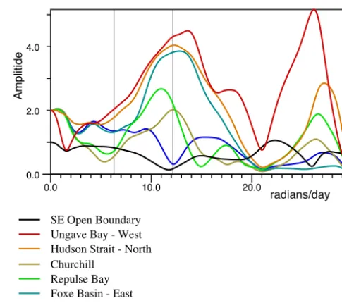
Figure 3. In colour: amplitude of the response function plotted
as a function of angular velocity for real values of angular veloc-ity. Colours: red, Ungava Bay (Hopes Advance Bay); orange, loca-tion R2 (see Fig. 1), north side of Hudson Strait; brown: Churchill; green, Repulse Bay; light blue, R3, East Foxe Basin; dark blue, R4, North Foxe Basin. In black: amplitude of outgoing (radiated) wave at boundary point R1.
Good depth data from Foxe Basin is limited, as it is cov-ered in ice for much of the year. Freely floating sea-ice should not affect the tidal wave. Sea-ice fixed to the shore should re-sult in increased turbulence and damping but is not expected to have a significant effect on wavelength.
This is because, as discussed in Webb (2011), with the fric-tion coefficient and depths used in the model, fricfric-tion has a significant effect on amplitudes and decay times but only a small effect on wavelength. Similarly, the use of a linear friction coefficient, instead of a fully nonlinear one, should affect decay times and amplitudes but have little effect on wavelength.
The suspicion therefore remains that the model phase er-rors result from a problem with the depths. No more can be done at this stage but the phase errors need to be kept in mind in the remainder of this analysis.
4 The response at real values of angular velocity
For the remainder of the study, the model was forced at the open boundary with an incoming wave of unit amplitude. Figure 3 shows the amplitude of the resulting model response at representative points within the region plus the amplitude of the outgoing wave at one point of the open boundary.
D. J. Webb: Tidal resonances of Hudson Strait 415
Table 1. Model M2 tidal amplitude (m) and phases (degrees relative to the equilibrium tide at Greenwich) compared with tide gauge analyses
(IHB, 1954).
Model Tide gauge
Amp. (m) Phase◦ Amp. (m) Phase◦
Hopes Advance Bay 69.6◦W 59.4◦N 3.16 13 3.88 10
Churchill 94.2◦W 58.8◦N 1.46 13 1.52 24
Great Whale River 77.8◦W 55.3◦N 0.54 345 0.63 17
Repulse Bay 86.5◦W 66.4◦N 1.63 18 1.88 192
Hall Beach 81.2◦W 68.8◦N 0.36 186 0.22 25
0.0 10.0 20.0 30.0
0.0 2.0 4.0
radians/day
Amplitide
SE Open Boundary
Ungave Bay - West
Hudson Strait - North
Churchill
Repulse Bay
Foxe Basin - East
Foxe Basin - Northeast
Fig. 3.In colour: amplitude of the response function plotted as a function of angular velocity for real values of
angular velocity. Colours: Red, Ungava Bay (Hopes Advance Bay); Orange, Location R2 (see Fig. 1), North
side of Hudson Strait; Brown: Churchill; Green, Repulse Bay; Light Blue, R3, East Foxe Basin: Dark Blue,
R4, North Foxe Basin. In black: amplitude of outgoing (radiated) wave at boundary point R1.
-5.0 0.0 5.0
-5.0 0.0 5.0
Real
Imaginary
Ungave Bay - West
0.0 0.5 1.0
-0.5 0.0 0.5
Real
Imaginary
SE Open Boundary
(a) Ungava Bay (b) Outgoing wave at R1
Fig. 4.Real and imaginary components of (a) the response function on the west side of Ungava Bay and (b) the
outgoing wave at point R1 on the open boundary, plotted for real values of angular velocity between zero and
30rad/day. Crosses at intervals of 10rad/day. The red sections correspond to the diurnal and semi-diurnal
tides. At zerorad/daythe response function at Ungava Bay has the value(2 +i0)and the outgoing wave has
the value(1 +i0).
on the western shore of Hudson Bay, but stations further south are omitted as the responses there are
180
similar to Churchill but with lower amplitudes.
Finally, the figure includes the outgoing wave at point R1 on the open boundary (see Fig. 2). This
8
Figure 4. Real and imaginary components of (a) the response function on the west side of Ungava Bay and (b) the outgoing wave at point
R1 on the open boundary, plotted for real values of angular velocity between zero and 30 rad day−1. Crosses at intervals of 10 rad day−1. The
red sections correspond to the diurnal and semi-diurnal tides. At zero rad day−1the response function at Ungava Bay has the value(2+i0)
and the outgoing wave has the value(1+i0).
the model semi-diurnal tides are highest. A station in north Foxe Basin is also included because the response there ap-pears to be very different to that of east Foxe Basin. In the south, the figure includes Churchill, on the western shore of Hudson Bay, but stations further south are omitted as the re-sponses there are similar to Churchill but with lower ampli-tudes.
Finally, the figure includes the outgoing wave at point R1 on the open boundary (see Fig. 2). This is chosen because it is in deep water at the foot of the continental slope and is in a position where it should give an indication of the be-haviour of Kelvin waves travelling south out of the model region. It also lies near the positions where the resonances, discussed later, show the maximum energy losses through the open boundary.
At zero angular velocity both the ingoing and outgo-ing waves at the open boundary have unit amplitude, so the amplitude everywhere equals two. As angular veloc-ity increases, the amplitudes initially tend to decrease but they then increase to maxima near the semi-diurnal tidal band. There is then a general decrease to minima around
21 rad day−13after which there are further maxima between 25 and 30 rad day−1.
Within this large-scale behaviour there are many individ-ual maxima and changes in curvature, which, on the basis of previous work, are likely to be due to individual resonances or groups of resonances. Sometimes the maxima and changes in curvature occur at the same angular velocity, indicating that such regions are coupled and affected by the same reso-nance. However, at other angular velocities the same regions may have very different response to the forcing.
A noticeable feature of the outgoing wave at R1 is that it has a minimum where the resonances are largest near 12 rad day−1 and a maximum near 22 rad day−1 where the large-scale response is least. It then has another minimum near 26 rad day−1where Ungava Bay has a maximum.
An alternative view of the system’s response is obtained by plotting the real and imaginary components of the response function, as in Fig. 4. As shown in Appendix A, the response functionR(x, ω)at positionxand angular velocityωcan be
3The paper uses units of radians per day (rad day−1). Thus the
semi-diurnal tides with periods around 12 h have angular velocities
around 4πrad day−1.
Fig. 5.Response function amplitude on the west side of Ungava Bay plotted as a function of complex angular
velocity. The colours denote complex phase, in degrees, as denoted on the scale below the main figure. Values
at real values of angular velocity are plotted in blue. The origin (0,0) is on the right with the positive real axis
(in red) running from right to left and the negative imaginary axis running into the figure. Both are marked
by red crosses every 1 rad/day. The vertical axis is marked similarly at unit intervals. On the real axis green
crosses indicate the limits of the tidal bands near2π(diurnal),4π(semi-diurnal),6πand8πrad/day.
Applying these ideas to Fig. 4, at Ungava Bay the response function is seen to contain four main
loop structures. These consist of two small loops generating the amplitude minima near 2 and 21
rad/dayand two larger ones which generate the maxima near 13 and 26rad/day.
The outgoing wave at R1 also shows large and small loops at roughly the same angular velocities,
220
but this time the large loops reduce the amplitude of the radiated wave. Near 12rad/daythe
ampli-tude drops to near 0.1, and as the radiated power depends on the square of the ampliampli-tude it implies
that the radiated power is close to 1% of the incident power.
5 The Response at Complex Values of Angular Velocity
The previous figures illustrate the type of information that can be obtained with models that can
225
investigate real values of angular velocity. However an advantage of the present model is that it
can also obtain solutions for complex values of angular velocity and thus explore the full resonant
structure of the system.
Figures 5 to 7 show the response function at four stations plotted on the complex plane. In these
figures the vertical coordinate indicates the response function amplitude and the colour represents
230
phase, zero phase being the phase of the incoming wave on the open boundary.
The functions can be interpreted using Eqn. 1. The poles in the complex plane correspond to the
resonances, the co-ordinate of the poles giving the real and imaginary components of each eigenvalue
ωj. The position of the resonances is the same in each figure but their strengths differ due to changes
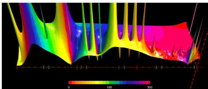
Figure 5. Response function amplitude on the west side of Ungava Bay plotted as a function of complex angular velocity. The colours
denote complex phase, in degrees, as denoted on the scale below the main figure. Values at real values of angular velocity are plotted in blue. The origin (0,0) is on the right with the positive real axis (in red) running from right to left and the negative imaginary axis running into
the figure. Both are marked by red crosses every 1 rad day−1. The vertical axis is marked similarly at unit intervals. On the real axis green
crosses indicate the limits of the tidal bands near 2π(diurnal), 4π(semi-diurnal), 6πand 8πrad day−1.
expressed as a sum over the resonance contributions, R(x, ω)=X
j
ψj(x)rj/(ω−ωj) , (1)
whereωj is the angular velocity of thejth resonance,ψj(x) describes the spatial structure of the resonance and rj de-pends on how the system is forced.
At a fixed location when the resonances are well sepa-rated, the response functionR(ω)near each resonances has the form
R(ω) = Aj/(ω−ωj)+B(ω) , (2) whereB(ω)represents the smooth background due to of dis-tant resonances.
When this function, without the background term, is plot-ted as in Fig. 4, its locus generates a simple circle. This starts at the origin whenω is minus infinity. It then moves in an anticlockwise direction, reaching maximum amplitude when
ωequalsωj, and returning to the origin asωapproaches in-finity.
When the background is added, isolated resonances gen-erate single loops on the smooth background. Where reso-nances are overlapping, more complicated structures may be formed but the contribution of each resonance still has the same simple underlying form.
Applying these ideas to Fig. 4, at Ungava Bay the response function is seen to contain four main loop structures. These consist of two small loops generating the amplitude minima near 2 and 21 rad day−1and two larger ones which generate the maxima near 13 and 26 rad day−1.
The outgoing wave at R1 also shows large and small loops at roughly the same angular velocities, but this time the large loops reduce the amplitude of the radiated wave. Near 12 rad day−1 the amplitude drops to near 0.1, and as
the radiated power depends on the square of the amplitude it implies that the radiated power is close to 1 % of the incident power.
5 The response at complex values of angular velocity
The previous figures illustrate the type of information that can be obtained with models that can investigate real val-ues of angular velocity. However, an advantage of the present model is that it can also obtain solutions for complex values of angular velocity and thus explore the full resonant struc-ture of the system.
Figures 5–7 show the response function at four stations plotted on the complex plane. In these figures the vertical coordinate indicates the response function amplitude and the colour represents phase, zero phase being the phase of the incoming wave on the open boundary.
The functions can be interpreted using Eq. (1). The poles in the complex plane correspond to the resonances, the coor-dinate of the poles giving the real and imaginary components of each eigenvalueωj. The position of the resonances is the same in each figure but their strengths differ due to changes in the eigenvectorψj(x)between locations.
D. J. Webb: Tidal resonances of Hudson Strait 417
Figure 6. The response function amplitude plotted as a function of complex angular velocity (a) at Churchill and (b) location R3 on the
eastern side of Foxe Basin. Colours and axes as in Fig. 5.
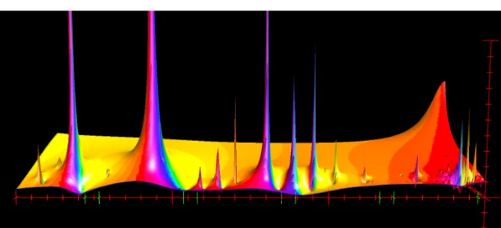
Fig. 7. Response function amplitude of the outgoing wave at point R1 on the open boundary. Colours and
scales as in Fig. 5.
5.1 Radiation at the Open Boundary
Figure 7 indicates that the first of the large loops in Fig. 4b is associated with resonances D to G and
280
the second large loop with resonance U. The first of the small loops is associated with the shelf and
Rossby wave resonances. The cause of the second loop is not so clear but it is likely to be Q together
with K and L.
In the previous study of the English Channel and Irish Sea (Webb, 2013a), the high semi-diurnal
tides in the Bristol Channel were found to result from two resonances which both had slightly higher
285
angular velocities. It was assumed that these were also responsible for the large amount of tidal
energy that was dissipated in the region.
The present result indicates that the strong absorption of tidal energy by the Hudson Bay system
is a result of four resonances which straddle the tidal band. The strong absorption thus may result
from straddling the tidal band or it may result from the fact that four resonances are involved, each
290
of which can provide an independent contribution to resonant absorption of tidal energy.
6 Structure of the Main Semi-Diurnal Resonances
The spatial structures of the four largest resonances near the semi-diurnal tidal band were calculated
using the method outlined in Appendix B2. The results are shown in Fig. 8. The solutions have been
normalised so that the maximum amplitude is one and the phase is zero in the west of Ungava Bay.
295
For two of the modes, the maxima are on the eastern side of Foxe Basin. The other two have maxima
on the western side of James Bay.
The energy flux vectors for resonance F are shown in Fig.9. This and similar plots (not included)
for the other modes show that, in each case, the flux is away from the deep regions of Hudson Strait,
13
Figure 7. Response function amplitude of the outgoing wave at point R1 on the open boundary. Colours and scales as in Fig. 5.
In Fig. 5, Ungava Bay is plotted because of the interest in its extreme tides and because the region appears to support a classic quarter-wavelength resonance. Churchill and location R3 (Fig. 6) are chosen to represent Hudson Bay and Foxe Basin. Location R1 (Fig. 7) lies beyond the outer edge of the continental slope and is chosen to capture any Kelvin wave progressing southward out of the model region.
In the limit of zero angular velocity, both the incoming and outgoing wave on the open boundary have unit amplitude. As a result, as shown in Figs. 5 and 6, the amplitude at the origin is two. Figure 7 shows only the outgoing wave on the boundary, so its amplitude at the origin is one.
As angular velocity increases along the real axis, the phase tends to increase. This arises because the ratio of the phase to the angular velocity is a measure of the time taken for the wave to propagate to each location from the forcing region. Off the real axis the behaviour is more complicated due to the phase increase of 2π radians close around each pole which arises from Eq. (2).
Starting from near the origin, there is initially a dense group of weak resonances which extends to near 6 rad day−1. As in Webb (2013a) these are the continental shelf and Rossby wave modes. There is then a series of gravity wave
modes extending to higher angular velocities. The angular velocities of these modes, calculated using the method out-lined in Appendix B2, are given in Table 2.
Near the real axis, the colours show that the phase at Un-gava Bay increases slowly, reaching 90◦in the region of the semi-diurnal tides. In contrast, there is a more rapid phase change at both Churchill and at location R3, the colours in-dicating that near the semi-diurnal band these phases are ap-proximately 450◦, i.e. one and a quarter wavelengths differ-ent from the forcing.
The response function for Ungava Bay shows that the large-amplitude region near the semi-diurnal tidal band (12 rad day−1) is associated with four main resonances.
These are resonances D to G of Table 2. The figures show that the same resonances are also responsible for large am-plitudes in Hudson Bay and Foxe Basin, the strength of in-dividual resonances there often being larger than in Ungava Bay.
In some ways this result is surprising. Ungava Bay is known to have high tides, and given the local bathymetry and distance from the shelf edge and the phase of the response function, the high semi-diurnal response might be expected to be due to a single quarter-wavelength resonance. Hudson
Resonance D Resonance E
File: gtide_D.h5
270.0 275.0 280.0 285.0 290.0 295.0 300.0 55.0
60.0 65.0 70.0
Longitude
Latitude
File: gtide_E.h5
270.0 275.0 280.0 285.0 290.0 295.0 300.0 55.0
60.0 65.0 70.0
Longitude
Latitude
Resonance F Resonance G
File: gtide_F.h5
270.0 275.0 280.0 285.0 290.0 295.0 300.0 55.0
60.0 65.0 70.0
Longitude
Latitude
File: gtide_G.h5
270.0 275.0 280.0 285.0 290.0 295.0 300.0 55.0
60.0 65.0 70.0
Longitude
Latitude
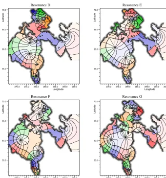
Fig. 8.The amplitude and phase of resonances D to G of table 2. Amplitudes normalised to one and phases are
relative to the west side of Ungava Bay. Thick lines are contours of amplitude at 0.1, 0.2, 0.4, 0.6 and 0.8. Thin lines are contours of phase at intervals of 30 degrees. Colours as in Fig. 1, with zero phase between the red and blue areas.
both eastwards towards the open boundary and westwards towards the high amplitude regions in 300
Foxe Basin or Hudson Bay.
None of the modes can be characterised by a single unique feature, such as a standing wave in
a limited region of shelf. Instead they appear to involve the coupling of a series of such simple or
underlying modes.
14
Figure 8. The amplitude and phase of resonances D to G of Table 2. Amplitudes normalised to one and phases are relative to the west side
of Ungava Bay. Thick lines are contours of amplitude at 0.1, 0.2, 0.4, 0.6 and 0.8. Thin lines are contours of phase at intervals of 30 degrees. Colours as in Fig. 1, with zero phase between the red and blue areas.
Bay and Foxe Basin are much further from the shelf edge and on the same basis they must involve at least three-quarter wavelength resonances and possibly one and a quarter wave-length resonances.
At higher angular velocities the Ungava Bay response function shows two further strong resonances. The first, res-onance Q near 21 rad day−1, has little impact on the response at real values of angular velocity. The second, resonance U near 27 rad day−1, has a much greater impact on the response in Ungava Bay. It is also responsible for an increased ampli-tude at Churchill but has essentially no impact at position R3. Further investigation of their structure showed that resonance Q is primarily a quarter-wavelength resonance of Cumber-land Sound and U a similar resonance of Frobisher Bay. 5.1 Radiation at the open boundary
Figure 7 indicates that the first of the large loops in Fig. 4b is associated with resonances D to G and the second large loop
with resonance U. The first of the small loops is associated with the shelf and Rossby wave resonances. The cause of the second loop is not so clear but it is likely to be Q together with K and L.
In the previous study of the English Channel and Irish Sea (Webb, 2013a), the high semi-diurnal tides in the Bris-tol Channel were found to result from two resonances which both had slightly higher angular velocities. It was assumed that these were also responsible for the large amount of tidal energy that was dissipated in the region.
D. J. Webb: Tidal resonances of Hudson Strait 419
270.0 275.0 280.0 285.0 290.0 295.0 300.0
55.0 60.0 65.0 70.0
Longitude
Latitude
0.0 0.5 1.0
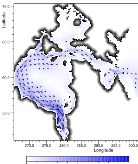
Figure 9. Energy flux vectors for resonance F. The flux is
nor-malised so that its maximum value is one.
6 Structure of the main semi-diurnal resonances
The spatial structures of the four largest resonances near the semi-diurnal tidal band were calculated using the method outlined in Appendix B2. The results are shown in Fig. 8. The solutions have been normalised so that the maximum ampli-tude is one and the phase is zero in the west of Ungava Bay. For two of the modes, the maxima are on the eastern side of Foxe Basin. The other two have maxima on the western side of James Bay.
The energy flux vectors for resonance F are shown in Fig. 9. This and similar plots (not included) for the other modes show that, in each case, the flux is away from the deep regions of Hudson Strait, both eastwards towards the open boundary and westwards towards the high-amplitude regions in Foxe Basin or Hudson Bay.
None of the modes can be characterised by a single unique feature, such as a standing wave in a limited region of shelf. Instead they appear to involve the coupling of a series of such simple or underlying modes.
The first of these is the quarter-wavelength resonance in-volving Ungava Bay. The justification for this is the fact that all four modes show an approximate 90 degree phase lag be-tween the west side of Ungava Bay and the shelf edge or open boundary – although depending on the precise point chosen the value can vary between 75 and 130 degrees.
A second is a three-quarter wavelength mode between the shelf edge or open boundary and the east side of Foxe Basin.
Table 2. Real and imaginary components of angular velocity (in
radians per day) for the gravity wave resonances.
Angular velocity Angular velocity
Real Imag. Real Imag.
A 4.1435 −1.1716 N 19.9437 −2.5796
B 5.1052 −1.6125 O 20.2071 −1.5208
C 7.5167 −1.2326 P 20.9670 −1.8545
D 9,4433 −1.5199 Q 21.4514 −2.1738
E 10.8327 −1.7144 R 23.2567 −1.6131
F 12.1613 −1.5320 S 24.4043 −1.3558
G 13.9215 −1.6782 T 26.1338 −1.6607
H 15.6169 −3.9629 U 26.5379 −1.2928
I 16.0036 −1.5008 V 27.7020 −2.0412
J 16.5089 −4.4841 W 28.7601 −1.1003
K 17.1372 −1.4164 X 28.9116 −1.7231
L 18.2980 −1.2522 Y 29.0517 −4.0404
M 19.7361 −1.5471
As seen best in resonance E where there is a maximum in Hudson Strait and a node to the north of Southampton Is-land, the locations lying roughly one-quarter and one-half of a wavelength from the open boundary.
A third is a half-wavelength resonance trapped between the northwest and southeast coasts of Foxe Basin. This is best seen in resonance D, but as the model had poor agree-ment with the measured tide in the NW of Foxe Basin, this possibility should be treated with caution.
Finally, Hudson Bay itself appears to support its own un-derlying mode, consisting of a single wavelength that circles the bay in an anticlockwise direction. This is best seen in resonance F.
The results imply that although resonances involving the shelf edge are important, the grouping of resonances around the semi-diurnal tides is partly due to standing waves within the interior of the Hudson Bay system.
7 Resonant contributions to the semi-diurnal tides
As discussed in Webb (2012), the response function near a tidal band can be split into the contribution of nearby reso-nances and a smooth background due to distant resoreso-nances. Thus,
R(x, ω)=X j
Aj(x)/(ω−ωj)+S(x, ω)+B(x, ω) , (3) whereR(x, ω)is the response function at positionxand an-gular velocityω. The sumj is over key nearby resonances andAj(x)is the residue atwj, the resonance angular veloc-ity. Methods for calculating the residue are described in Ap-pendix B3. For this part of the analysis, the symmetry term
S(x, ω), due to the mirror images of the resonances in the summation, is simple to calculate and so is split off from the background.
-4.0 -2.0 0.0 2.0 0.0
2.0 4.0
Real
Imaginary
Ungave Bay - West
D
E
F
G D
E
F
G
0.0 0.5 1.0
0.0 0.5
Real
Imaginary
SE Open Boundary D
E
F
G
D
E
F G
(a) Ungava Bay (b) Outgoing wave at R1
Fig. 10.In black: real and imaginary components of the response function (a) on the west side of Ungava Bay
and (b) the outgoing wave at point R1 on the open boundary, plotted for real values of angular velocity between
11 and 14rad/day. Coloured vectors indicate the contributions of the resonances D to G of table 2 and their
conjugates. The blue line is the residual background. The red section of the main curve corresponds to the
semi-diurnal tides.
tide in the NW of Foxe Basin, this possibility should be treated with caution.
315
Finally, Hudson Bay itself appears to support its own underlying mode, consisting of a single
wavelength that circles the bay in an anti-clockwise direction. This is best seen in resonance F.
The results imply that although resonances involving the shelf edge are important, the grouping
of resonances around the semi-diurnal tides is partly due to standing waves within the interior of the
Hudson Bay system.
320
7 Resonant Contributions to the Semi-Diurnal Tides
As discussed in Webb (2012), the response function near a tidal band can be split into the contribution
of nearby resonances and a smooth background due to distant resonances. Thus,
R(x,ω) =X j
Aj(x)/(ω−ωj) +S(x,ω) +B(x,ω), (3)
whereR(x,ω)is the response function at positionx and angular velocityω. The sumj is over
325
key nearby resonances andAj(x)is the residue atwj, the resonance angular velocity. Methods for
calculating the residue are described in Appendix B3. For this part of the analysis, the symmetry
termS(x,ω), due to the mirror images of the resonances in the summation, is simple to calculate
and so is split off from the background.
In Fig. 10, Eqn. 3 has been used to determine how the four resonances of Fig. 8 contribute to
330
the high semi-diurnal tides of Ungava Bay and the low outgoing wave at position R1 on the open
boundary.
16
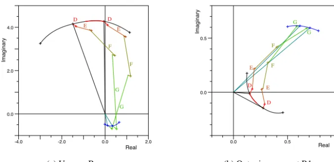
Figure 10. In black: real and imaginary components of the response function (a) on the west side of Ungava Bay and (b) the outgoing wave
at point R1 on the open boundary, plotted for real values of angular velocity between 11 and 14 rad day−1. Coloured vectors indicate the
contributions of the resonances D–G of Table 2 and their conjugates. The blue line is the residual background. The red section of the main curve corresponds to the semi-diurnal tides.
In Fig. 10, Eq. (3) has been used to determine how the four resonances of Fig. 8 contribute to the high semi-diurnal tides of Ungava Bay and the low outgoing wave at position R1 on the open boundary.
It shows that in Ungava Bay the high tides are primarily due to resonances F and G. They both have large amplitudes and, as their phases are similar, they reinforce each other. Resonance E makes some contribution, but D is insignificant, its amplitude being smaller than the background.
Resonances F and G are also the dominant ones at position R1. At 12 rad day−1they both have the effect of reducing the amplitude of the outgoing wave by about a third. At the same point resonances D and E are contributing to a reduction of the outgoing wave, but by 13 rad day−1this is no longer the case.
The net effect of the resonances at 12 rad day−1 is to re-duce the response function amplitude from 0.91 to 0.15. Assuming that the power is proportional to the amplitude squared, this means that the four resonances are absorbing over 97 % of the incident tidal energy. Resonances F and G together reduce the energy by approximately 90 % and al-though the contributions of resonances D and E are much smaller they are responsible for absorbing over 70 % of the remaining energy.
8 Conclusions
The study has shown that the semi-diurnal tides of the Hud-son Bay region are dominated by four reHud-sonances. These straddle the semi-diurnal tidal band and contribute both to high tidal amplitudes within the region and to very low am-plitudes in the tidal wave radiated away from the region.
The previous study, made using a time-dependent model (Arbic et al., 2007), was only able to identify one resonance affecting the semi-diurnal tides. The new result therefore em-phasises the usefulness of the present approach.
The study does not explain why the Hudson Bay system is such a good absorber of tidal energy and more effective than the English Channel and Irish Sea but it does give hints that need to be followed up.
The first is the primary result that the Hudson Bay system has four significant resonances close to and straddling the semi-diurnal tidal band. In the case of the Bristol Channel and Gulf of St Malo there are only two resonances and they lie to one side of the tidal band.
The study also used one of the points on the open boundary as an analogue of the reflected wave for the case of a uniform amplitude incident wave at all points on the open boundary. Although the uniform amplitude incident wave is a special case, it is a plausible first approximation to the way the M2 tide forces the region.
The results show that each of the four main resonances acted to reduce the amplitude of the reflected wave in the semi-diurnal tidal band. At 4πrad day−1, two of the
reso-nances together absorbed∼90 % of the incident energy and the other two, although weaker, absorbed∼70 % of the re-mainder. The small reflection coefficients imply that all four resonances have impedances which are well matched to that of the deep ocean.4
The study shows that the closeness of the resonances is partly due to the complex topography of the region. As well as the “classical” 1/4 wavelength wave between Ungava Bay and the shelf edge, the deep Hudson Strait also allows the de-velopment of 3/4 wavelength, and possibly 5/4 wavelength,
4Impedance matching is critical in the design of waveguides and
D. J. Webb: Tidal resonances of Hudson Strait 421
resonances between the shelf edge and features far to the west. There, both Foxe Basin and Hudson Bay are of the right size to support standing waves of near-tidal period.
The depth of Hudson Strait also means that energy dissi-pation is reduced compared with a normal shelf. The mean depth (∼300 m) is approximately four times that of a normal shelf (∼80 m), so the frictional effect per wavelength in the strait should be halved. This probably helps in matching the Foxe Basin and Hudson Bay components of the resonances to the deep ocean.
The effectiveness of a continental shelf region in absorbing tidal energy is also likely to depend on both the length of con-tinental shelf involved and the angle at which the tidal wave
approaches the shelf. These features have not been studied here but as it passes the English Channel and Irish Sea, the semi-diurnal tidal wave in the deep ocean runs roughly par-allel to the shelf edge. In contrast, as it approaches Hudson Strait the wave approaches roughly at right angles to the shelf edge.
To conclude, the present study has given new insights into the properties of the Hudson Bay region and the complex interactions that are involved. The study has shown that there is still much to be learnt about the physics of the region but the results presented here should provide a useful basis for further work.
Appendix A: Solution in terms of resonances
Laplace’s tidal equations with a linear friction term are
ρ∂u/∂t+ρf×u+ρg∇η+(κ/ h)u = ρg∇η0, (A1) ∂η/∂t+ ∇ ·(hu) = 0,
whereuis horizontal velocity, ηtidal height,ρ density, f the Coriolis parameter, ggravity, hwater depth, κ the lin-ear coefficient of bottom friction andη0the equilibrium tide
forcing the ocean.
If u(x, t )andη(x, t )at locationx and time t are repre-sented by the vector9,
9(x, t )=
u(x, t ) η(x, t )
, (A2)
and if 90(x, t )=
0
η0(x, t )
, (A3)
then the tidal equations can be written in the form
∂9(x, t )/∂t+L9(x, t )=L90(x, t ) (A4)
where L is a matrix operator discussed further in Webb (2014).
Consider the response when the system is forced at angular velocityω. The solution will then have the form
9(x, t ) = (9(x, ω)exp(−iωt )+c.c. , (A5) = 2Re(9(x, ω)exp(−iωt )) , (A6) whereRe()represents the real part andc.c.represents com-plex conjugate. Substituting in Eq. (A4),
(L−iω1)9(x, ω)=L90(x, ω) , (A7) where90(x, ω)and9(x, ω)are the forcing and ocean re-sponse at angular velocityωand 1 is the unit matrix.
Equations of this form can be solved using the eigenfunc-tions of the operatorLand its adjointL. The basic method ise described in Morse and Feshbach (1953). Webb (2014) dis-cusses its application to Laplace’s tidal equations and shows how a suitable definition of the inner or dot product generates a physically meaningful adjoint.
Dropping thexcoordinate, ifωjandψjare the eigenval-ues and eigenfunctions of the equation
(L−iωj1)ψj =0 (A8)
and ifλk andφk are the eigenvalues and eigenfunctions of the adjoint operator
(Le−iλk1)φk=0, (A9)
then (Morse and Feshbach, 1953; Webb, 2014) Z
dx φ∗j(x)·ψk(x)(ωj+λk)=0. (A10)
Thus eitherλk equals−ω∗j or the integral is zero, so the eigenfunctions are orthogonal.
Normalise ψk(x)so that the above integral with φk(x) equals one. Then expanding9(x, ω)and the equilibrium tide 90(x, ω)in terms of the eigenfunctions
9(x, ω) = X j
aj(ω)ψj(x), (A11)
90(x, ω) = X j
ψj(x) Z
dx0φ∗j(x0)·90(x0, ω). (A12)
Substituting in Eq. (A7),
(L−iω)X
j
aj(ω)ψj(x)=
LX j
ψj(x) Z
dx0φ∗j(x0)·90(x0, ω),
X
j
aj(w)(iωj−iω)ψj(x)=
X
j
ψj(x)iωj Z
dx0φ∗j(x0)·90(x0, ω). (A13)
Multiplying byφ∗k(x)and integrating overx,
ak(ω)=(−ωk/((ω−ωk)) Z
dx0φ∗k(x0)·90(x0, w). (A14)
Thus the solution to Eq. (A4) is 9(x, ω)=
X
j ψj(x)
−wj
w−wj Z
dx0 φ∗j(x0)·90(x0, ω). (A15)
In the type of problem investigated in this paper, the forc-ing term90(x, t )can be separated into a spatial term90(x)
and a time-dependent term 90(t ), with Fourier transform 90(ω). Then,
9(x, ω) = R(x, ω)90(ω) , (A16)
R(x, ω)is the (vector) response function R(x, w) = X
j ψj(x)
rj
w−wj
(A17)
rj = −ωj Z
dx0 φ∗j(x0)·90(x0) . (A18) The response functions plotted in Figs. 5 and 6 are the sea surface elevation component ofR.
A1 Forcing at an open boundary
D. J. Webb: Tidal resonances of Hudson Strait 423
replaced by a function which is zero within the region stud-ied but has a step change along a line just inside the open boundary,
η0(x)= −2(n)ηb(s), (A19)
wherenands are the coordinates normal and tangential to each point on the open boundary andηb(s)is the forced wave at positions. The function2is zero inside the boundary and equals one on and outside the open boundary.
To confirm that Eq. (A19) has the right form, integrate Eq. (A1) between a point a distancewithin the region and a point on the boundary. As the distancetends to zero, all terms tend to zero except for
0 Z
−
dn ρg(∂/∂n)η= −
0 Z
−
dn ρg(∂/∂n)2(n)ηb(s). (A20)
Butηis zero on the boundary and the integral of the gra-dient of a step function is one, so after integrating and rear-ranging, the value of sea level just inside the boundary equals
η=ηb(s), (A21)
as required.
The derivation of Eq. (A15) follows as before, the main change occurring in Eq. (A13) which now reads as
(L−iω1)X
j
aj(ω)ψj(x) = −
g∇(2(n)ηb(s))
0
.
(A22)
When multiplied byφ∗k(x)and integrated overx, the right-hand side becomes an integral around the open boundarys,
−g I
ds φkn∗(x(s))·(∂/∂n)(2(n)ηb(s)), (A23)
whereφknis the velocity component of eigenvectorφkwhich is normal to the boundary. Integrating by parts, this becomes
g I
ds ∂/∂n(φkn∗(x(s)))·ηb(s). (A24) Thus the integral of Eq. (A15) is replaced by an integral around the open boundary.
A2 Symmetry
Equation (A5) corresponds to a Fourier transform represen-tation when only a single angular velocity is present. For the general case where the system contains a full range of an-gular velocities, the Fourier transform between the time and angular velocity representation of9(x)is
9(x, t ) = ∞ Z
−∞
dω exp(−iω t )9(x, ω), (A25)
9(x, ω) = 1 2π
∞ Z
−∞
dt exp(iω t )9(x, t ). (A26)
9(x, t )is real so
9(x,−ω∗)∗ = 1 2π
∞ Z
−∞
dt exp(iω t )9(x, t ), (A27)
and
9(x,−ω∗)∗ = 9(x, ω) . (A28)
90(x, t )is also real, so
90(x,−ω∗)∗ = 90(x, ω) . (A29)
Similarly, for the response function R(x, ω) relating 9(x, ω)and90(x, ω),
R(x,−ω∗)∗ = R(x, ω) . (A30)
In Eqs. (A15) and (A17), this means that if there is a pole atωjwith residuerj(x), there must also be one at−ω∗j with residue−rj(x)∗.
A3 Causality
Substituting the response function equation (Eq. A16) into Eq. (A25),
9(x, t ) = ∞ Z
−∞
dω exp(−iω t )9(x, ω) (A31)
= ∞ Z
−∞
dω exp(−iω t )R(x, ω)90(ω), (A32)
= ∞ Z
−∞
dω exp(−iω t )R(x, ω) 1
2π ∞
Z
−∞
dt0 exp(iωt0)90(t0). (A33)
Let the forcing90(t )be an impulse at time zero only. Such an impulse can be represented by the product90δ(t ).90is a constant and the delta functionδ(t )has the property that for any functionF (t ),
Z
dt δ(t )F (t )=F (0). (A34)
Then, using Eq. (A17),
9(x, t ) = ∞ Z
−∞
dω exp(−iω t )X
j ψj(x)
rj
w−wj 1 2π ∞
Z
−∞
dt0 exp(iω t0)δ(t0)90 (A35)
= 1
2π ∞ Z
−∞
dω exp(−iωt ))
X
j ψj(x)
rj
w−wj
90. (A36)
The integrand is an analytic function ofω, so the integral can be completed using the method of contour integration. If t is positive, exp(−iωt )tends to zero asωtends to mi-nus infinity, so the contour can be completed in a clockwise direction around the negative imaginary half-plane. Thus, 9(x, t ) = −iX
j
exp(−iωjt )ψj(x)rj90, (A37)
where the sum is over the poles in the negative imaginary half plane. Each resonance oscillates independently and dies away at its own natural rate.
Ift is negative, the contour can be completed around the positive imaginary half-plane. If there are any poles there, the result is non-zero, so the system is responding before any forcing is applied. This is impossible for physically realistic systems as it breaks causality. As a result there can be no poles in the positive imaginary half-plane, i.e. no resonances with positive imaginary components of angular velocity.
Appendix B: Mathematical and numerical details
The model used for the present study represents Laplace’s tidal equations as a set of finite difference equations on an Arakawa C-grid, as described in Webb (2013a). The model assumes a time dependence of the form exp(−iωt ), wheret
is time andωthe angular velocity of the ocean wave. If the model variables are represented by a vectory, then the finite difference equations can be written as a matrix equation,
(L−iω1)y=z, (B1)
where 1 is the unit matrix. The term (−iω1)results from the time-dependent terms in Laplace’s tidal equations and the matrix L contains the contributions from all the other terms in the set of finite difference equations. The vectorz repre-sents the forcing. If the variables are numbered in a system-atic manner, L becomes a band matrix and the equations can be solved using efficient band matrix algorithms.
B1 The open boundary condition
In previous versions of the model, sea surface height (SSH) points on the open boundary were treated explicitly as part of the model vectory. However, an investigation of the prop-erties of the adjoint system (Webb, 2014) showed that it was better to treat the open boundary condition implicitly, that is as an additional term acting on the normal velocities at points adjacent to the open boundary.
Webb (2014) also showed that it is better to set the tan-gential velocities at the open boundary to zero, so this was done in the present model. The change ensures that the finite difference Coriolis terms conserve energy and also ensures that the resulting matrix equation has the expected adjoint symmetry.
The previous model also used Dirichlet boundary condi-tions in which SSH on the open boundary is fixed. To allow radiation of energy through the open boundary, a scheme has been developed based on the one proposed by Flather (1976) which is often used for time-dependent models.
Letζ represent sea surface height anduthe velocity nor-mal to an open boundary placed at the origin of coordinatex. In a plane wave propagating in the positive direction in a re-gion of constant depthh, the sea surface height and velocity are related by
u = (c0/ h)ζ, (B2)
where the wave speedc0equals(gh)1/2.
The new boundary condition assumes that the solution in the neighbourhood of a boundary point can be expressed as the sum of two such waves each propagating in opposite di-rections normal to the boundary,
ζ = Aexp(ikx−iωt )+Bexp(−ikx−iωt ), (B3)
u = A(c0/ h)exp(ikx−iωt )−B(c0/ h)exp(−ikx−iωt ).
If A represents the unknown outgoing wave and B the known incoming wave, then eliminatingA, the open bound-ary condition becomes
ζ−(c0/ h)u = 2B. (B4)
As the open boundary value ofζ is not part of the model vector, this equation is used to replace the term involving the open boundaryζin the equation for the normal velocity point closest to the boundary.
D. J. Webb: Tidal resonances of Hudson Strait 425
B2 Calculation of eigenvalues and eigenvectors
Initial estimates of the eigenvalues ωj were obtained from the data sets used to generate Figs. 5 and 6 by fitting the four points around each maximum of the response function, for a fixedxk, to the expansion
R(xk, ω) = Rj(xk)/(ω−ωj)+B(xk)+C(xk)ω. (B5) Accurate values of the eigenvector and eigenvalue were then obtained by inverse iteration, i.e. by solving the set of equations
(L−iω0j1)ψ[jn]=ψj[n−1]/Nj[n−1], (B6) whereωj0 is the initial estimate ofωj,ψ
[n]
j is the solution following thenth iteration andNj[N]is a normalising constant equal to the maximum element of vectorψ[jn].
The sequence converged to the order of the machine rounding error after less than 10 iterations. Then ifψj is the converged eigenvector andNj the converged normalisation constant,
(L−iωj1)ψj = 0. (B7)
(L−iω0j1)ψj = ψj/Nj.
Subtracting the equations, the true eigenvalueωis given by
ωj = ωj0 −i/Nj. (B8)
The results were checked by obtaining the correspond-ing eigenvectorsφjof the Hermitian adjoint matrix equation with eigenvalue −w∗j. These were then normalised so that the dot product (ψ∗j·φj)equalled one. Under these condi-tions the dot product(ψ∗j·φk)should be zero whenj6=k. This was found to be correct to within the machine rounding error.
B3 The residue
In Sect. 7 of the paper, Eq. (3) requires the SSH residue
Aj(xm)of the eigenvector at positionxm. Lety be the so-lution of the matrix equation B1,
y = X
k
akψk. (B9)
Then using the matrix eigenvectors and eigenvalues de-fined in Appendix B2,
(L−iω1)X
k
akψk = z, (B10)
X
k
ak(iωk−iω)ψk = z. (B11)
Taking the dot product withφjand rearranging,
aj =
i (ω−ωj)
(φ∗j·z) . (B12)
Thus the residue atxmis
Aj(xm) = ψj,mi(φ∗j·z) . (B13) The residue can also be obtained from the inverse iteration sequence (Eq. B6) without solving for the adjoint eigenvalue. If the iterations are initialised withψ[j0]equal tozandNj[0]
equal to 1, then afterniterations ψj[n]=ψj[n−1]i(φ∗j·z)
n Y
k=1
(Nj[k]/Nj[n])+, (B14)
whereis the contribution from other resonances. Once the solution has converged then, to within the machine rounding error,is zero andψ[jn]equalsψ[jn−1], so
i(φ∗j·z) = n Y
k=1
(Nj[n]/Nj[k]), (B15)
Aj(xm) = ψj,m n Y
k=1
(Nj[n]/Nj[k]). (B16)
Acknowledgements. I wish to acknowledge the support of the
Marine Systems Modelling group of the United Kingdom’s Na-tional Oceanography Centre. The group provided essential material support for this research and also funded publication of the results. Thanks also to the reviewers for their detailed comments.
Edited by: N. Wells
References
Arbic, B. K., St-Laurent, P., Sutherland, G., and Garrett, C.: On the resonance and influence of the tides in Ungava Bay and Hudson Strait, Geophys. Res. Lett, 34, L17606, doi:10.1029/2007GL030845, 2007.
Courant, R. and Hilbert, D.: Methods of Mathematical Physics, Vol-ume 1, John Wiley & Sons, 2008.
Egbert, G. D. and Erofeeva, S. Y.: Efficient Inverse
Modeling of Barotropic Ocean Tides, J. Atmos.
Oceanic Technol., 1919, 183–204,
doi:10.1175/1520-0426(2002)019<0183:EIMOBO>2.0.CO;2, 2002.
Egbert, G. D. and Ray, R.: Estimates ofM2tidal energy dissipation
from TOPEX/Poseidon altimeter data, J. Geophys. Res., 106, 22475–22502, 2001.
Flather, R. A.: A Tidal Model of the North-west European Conti-nental Shelf, Mémoires Société Royale des Sciences de Liége, 10, 141–164, 1976.
Fong, S. and Heaps, N.: Note on the quarter-wave tidal resonance in the Bristol Channnel, Institute of Oceanographic Sciences, Re-port No., 63, 15 pp., 1978.
Hunter, J. R.: A Note on Quadratic Friction in the Presence of Tides, Est. Coast. Mar. Sci., 3, 473–475, 1975.
Huthnance, J. M.: On shelf-sea resonance with application to Brazilian M3 tides, Deep Sea Res., 27A, 347–366, 1980. IHB: Tides, List of Harmonic Constants, Special Publication
No. 26, International Hydrographic Bureau, Monaco, 1954. IOC, IHO, and BODC: Centenary Edition of the GEBCO
Digi-tal Atlas, published on CD-ROM on behalf of the Intergovern-mental Oceanographic Commission and the International Hydro-graphic Organization as part of the General Bathymetric Chart of the Oceans, British Oceanographic Data Centre, Liverpool, UK, 2003.
Le Provost, C. and Rougier, F.: Energetics of the barotropic ocean tides: An estimate of bottom friction dissipation from a hydrody-namic model, Progr. Oceanogr., 40, 37–52, 1997.
Mathews, J. and Walker, R. L.: Mathematical Methods of Physics, W. A. Benjamin, Inc., 1965.
Miller, G. R.: The flux of tidal energy out of the deep ocean, J. Geophys. Res., 71, 2485–2489, 1966.
Morse, P. M. and Feshbach, H.: Methods of Theoretical Physics: Volume 1, McGraw-Hill, 1953.
O’Reilly, C. T., Solvason, R., and Solomon, C.: Where are the World’s Largest Tides, in: BIO Annual Report: 2004 in Review, edited by: Ryan, J., 44–46, Biotechnol. Ind. Org., Washington, DC, 2005.
Riley, K. F., Hobson, M. P., and Bence, S. J.: Mathematical meth-ods for Physics and Engineeering, Cambridge University Press, 1998.
Webb, D. J.: Green’s Function and Tidal Prediction, Rev. Geophys. Space Phys., 12, 103–116, 1973.
Webb, D. J.: A Model of Continental Shelf Resonances, Deep-Sea Res., 23, 1–15, 1976.
Webb, D. J.: Tides and Tidal Energy, Contemporary Physics, 23, 419–442, 1982.
Webb, D. J.: Notes on a 1-D Model of Continental Shelf Reso-nances, Research and Consultancy Report 85, National Oceanog-raphy Centre, Southampton, available at: http://eprints.soton.ac. uk/171197 (last access: 19 May 2014), 2011.
Webb, D. J.: On the shelf resonances of the Gulf of Carpentaria and the Arafura Sea, Ocean Sci., 8, 733–750, doi:10.5194/os-8-733-2012, 2012.
Webb, D. J.: On the shelf resonances of the English Channel and Irish Sea, Ocean Sci., 9, 731–744, doi:10.5194/os-9-731-2013, 2013a.
Webb, D. J.: On the Impact of a Radiational Open Boundary Con-dition on Continental Shelf Resonances, National Oceanogra-phy Centre, Internal Document 06, National OceanograOceanogra-phy Cen-tre, Southampton, available at: http://eprints.soton.ac.uk/349401 (last access: 19 May 2014), 2013b.