TOKI Compression for Plasma Particle Simulations

(1)

TOKI Compression for Plasma Particle Simulations

∗

)

Katsumi HAGITA, Hiroaki OHTANI

1)

_{, Tsunehiko KATO}

2)

_{and Seiji ISHIGURO}

1) National Defense Academy, 1-10-20 Hashirimizu, Yokosuka 239-8686, Japan

1)_{National Institute for Fusion Science, 322-6 Oroshi-cho, Toki 509-5292, Japan}

2)_{Hiroshima University, 1-3-1 Kagamiyama, Higashi-Hiroshima 739-8526, Japan}

(Received 19 December 2013/Accepted 28 April 2014)

We propose a TOKI (Time Order, Kinetic, and Irreversible) compression method for recording smooth tra-jectories of particles from PIC (electromagnetic particle-in-cell) simulations. In a TOKI compression, instead of storing entire time sequences of particle positions, we store particle trajectories in terms of coefficients of approximating polynomials. In the current implementation, these coefficients are determined either by the least-squares method or by the Chebyshev approximation formula to obtain quasi-minimax polynomials. In this paper, we present the technique of TOKI compression and compare it with other lossy compression schemes, such as XTC. Comparisons are made using data from a PIC simulation for 150,000 electrons and 150,000 ions. For smooth trajectories, the compression ratio by TOKI is better than that by the XTC format. However, for ballistic trajectories, the compression ratio by TOKI is not good because of the significant overhead in storing raw values of trajectories. We also found that the compression efficiency for ion trajectories is better than that for electron trajectories. This is attributed to different characteristic time scales of motions due to the difference in mass. We expect that the behavior of the compression ratio in TOKI can be used to characterize motions of plasma particles.

c

2014 The Japan Society of Plasma Science and Nuclear Fusion Research

Keywords: TOKI compression, plasma particle simulation, visualization, smooth animation DOI: 10.1585/pfr.9.3401083

1. Introduction

Large-scale simulations in fusion science are now be-ing extensively performed thanks to recent progress in computer power. We can perform plasma particle simula-tions with billions of particles by the PIC (electromagnetic particle-in-cell) method [1]. However, in these large-scale simulations, recording particle data (e.g., trajectories) re-quires massive storage, which has become a serious prob-lem because improvements in performance of data stor-age devices have been much slower than improvements in computer power. Hence, observations of large-scale sim-ulation results, such as the detailed behavior of particles, require much more eﬀort than previous simulations. For such situations, we propose an improvement by compress-ing trajectory data. To achieve a high compression ratio, we approximate the trajectory of a particle by piecewise polynomials and store the coeﬃcients of the polynomials instead of storing the entire time sequence of particle posi-tions. We call this scheme the TOKI (Time Order, Kinetic, and Irreversible) compression method.

The basic concepts of TOKI are as follows. (i) The trajectory of each particle can be approximated by piece-wise polynomials, provided the trajectory is divided into appropriate subregions. (ii) In each subregion, the trajec-tory is approximated by a polynomial, so the behavior of

author’s e-mail: [email protected]

∗)_{This article is based on the presentation at the 23rd International Toki} Conference (ITC23).

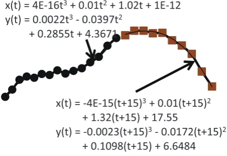
Fig. 1 Illustration of a particle trajectory in two dimensions (points) and curves ﬁt by TOKI compression to third-degree polynomials.

the trajectory is captured by the coefficients of that poly-nomial. For example, if we use third-degree polynomi-als for approximation, only four coefficients are needed to represent the trajectory in a subregion. This can be an ef-ficient (lossy) compression method for particle trajectory data. (iii) Subregions are determined so that the error be-tween the original trajectory and the polynomial approx-imation is below a predetermined value that ensures the accuracy of the approximation.

As a brief explanation of the concept of TOKI, Fig-ure 1 shows an illustration of a particle trajectory in two

c

2014 The Japan Society of Plasma

(2)

dimensions and the fitted curves obtained by TOKI com-pression. In this figure, the trajectory is divided into two intervals and each interval is fit by a third-degree polyno-mial. Division of the trajectory into intervals is needed to keep the maximum error between the data and the fitted curve (polynomial) below a given tolerance. (In the figure, the first interval corresponds to the time ranget = 0 - 14 and the second interval to the ranget=15 - 24.) In the first interval, 15 points are replaced by the values of four coeffi -cients in the third-degree polynomial; this is data compres-sion.

Plasma is a quasi-neutral gas of charged and neutral particles that exhibit collective behavior [2]. In plasma, magnetic reconnection is an interesting phenomenon. Dur-ing magnetic reconnection, the topology of magnetic ﬁeld lines changes on a macroscopic scale and global plasma transport takes place. In this process, the frozen-in mag-netic ﬁeld line condition is broken due to microscopic ef-fects, such as kinetic and particle-wave interactions. To un-derstand the role of the microscopic trigger, such as com-plex individual motions of unmagnetized particles, exten-sive PIC simulations have been performed [3–5].

In space physics and astrophysics, there are also many important phenomena associated with kinetic collisionless plasmas. One example is the particle acceleration process in collisionless shocks; it is widely believed that in super-nova remnants, cosmic rays with energies below 1015 eV are accelerated in collisionless shocks. Generally, these acceleration processes are kinetic and stochastic, and only a small fraction of particles are selectively accelerated to high energies. These processes have been studied with kinetic plasma simulations, and recent large-scale simula-tions show that some kind of acceleration processes indeed occur in collisionless shocks [6–8]. To investigate these processes in detail, it is essential to understand the acceler-ation histories of individual particles. For this purpose, it is desirable to record time sequences (histories) of positions, momenta, and energies for as many accelerated particles as possible and subsequently analyze them.

To study such related detailed motions, it is necessary to record the positions of all plasma particles at high sam-pling rates. In addition, smooth animations are expected to be one useful tool for analyzing complex plasma phenom-ena.

To eﬃciently record time sequences of positions, namely trajectories, a compression technique is necessary. As a versatile compression method, HDF-5 is widely used in various areas of computational simulation. HDF-5 is a hierarchical data format originally developed at the Na-tional Center for Supercomputing Applications. It is cur-rently supported by the HDF Group [9]. HDF-5 is a set of ﬁle formats and libraries to store and organize large amounts of numerical data.

In compressed data, part of the ﬁle is occupied by ran-dom values smaller than the precision required for loss-less compression. For molecular dynamics simulations of

molecules, such as proteins, the XTC format is a portable format used as a lossy compression method [10, 11]. Tra-jectories are written using a reduced-precision algorithm that works in the following way: coordinates are multi-plied by a scale factor (typically 1000) and then rounded to integer values. The algorithms for XTC are based on the observation that diﬀerences in atomic coordinates and ve-locities, in either time or space, are generally smaller than the absolute values of the coordinates and velocities them-selves [12]. This is considered to be lossy compression with the elimination of random values that are less than the required precision; the result is suitable for smooth an-imations.

In the TOKI compression scheme, particle trajectory data are compressed with following features [13]:

· A particle trajectory is approximated by piecewise polynomial functions whose basis is related to the characteristic motion of the particle.

· The diﬀerence between the original trajectory and the polynomial approximation is guaranteed to be smaller than a given allowable constant. To ensure this, direct checks should be performed in an encoder.

· Time-sequence data of trajectories are treated inde-pendently for each particle. Thus, the divisions of tra-jectories into intervals are not the same for diﬀerent particles.

In Section 2, we present the basic procedure used in a TOKI compression, and we describe the PIC simula-tion performed to obtain test data. Secsimula-tion 3 presents re-sults from TOKI implementations with the least-squares method and preliminary results with Chebyshev approxi-mation. Compression ratios from TOKI and XTC com-pression are compared for various sampling rates. Section 4 concludes the paper.

2. Method

2.1 TOKI compression with least-squares

method

In the TOKI compression algorithm, we seek the longest interval over which the original trajectory can be approximated by a kth-degree polynomial within an al-lowed (given) errorε.

maxsj+lj−1

i=sj

xi−

k

n=0an,jt

n

i< ε. (1)

Here, {xi} denotes a time series of positions for a certain

particle at timesi, whilesjandljare the starting time and

length (number of data points) of the jth interval, respec-tively. The quantitiesan_,jare coeﬃcients of thekth-degree

polynomial used for approximation in the jth interval. To reduce the ﬁle size, we record these coeﬃcients,an_,j,

in-stead of {xi}. When Eq. (1) is not satisﬁed for a minimum

interval length, we record {xi} directly. Hence, the error

(3)

In our first implementation, we use the least-squares method to find the coefficients of thekth-degree polyno-mial in a certain interval (for ease of development of test codes). With the least-squares method,

sj+lj−1

i=sj

xi−

k

n=0an,jt

n i

2

→min, (2)

we obtain values for the coeﬃcientsan,j. Then, we check

whether the condition (1) is satisﬁed. When it is not even for the minimum interval length, we store {xi} directly.

The above procedure is performed in a work array. Here we present a brief explanation of the work array of lengthLwork.

1) The trajectory data for a selected particle are stored in a work array. Here, the number of stored values is

Lwork.

2) We ﬁt the trajectory by a polynomial with the least-squares method (2) for the data in the work array whose length isLwork. Using the obtained ﬁtting pa-rametersan,j, we check condition (1).

3) When the condition (1) is satisﬁed, the parametersan,j

are recorded, then we move to step 1 for the next time sequence.

4) When condition (1) is not satisﬁed, we divide the interval in half and repeat the ﬁtting with the least-squares method (2) for the data whose length is now

Lwork/2. Using the obtained ﬁtting parametersan_,j, we

check condition (1).

5) When condition (1) is satisﬁed, we increase the length of the interval to seek the longest interval that can be represented by the approximation polynomial while satisfying (1). Otherwise, we decrease the length. 6) As a result, we obtain the longest interval and

coef-ﬁcientsan_,jfor that interval while preserving (1).

Fi-nally, these coefficients are recorded in a file. Then we move to step 1 for the next time sequence. The length Lwork of the work array limits the maximum interval for compression. Therefore, the size of the work array can significantly affect the efficiency of the compres-sion. For example, consider a data set with 1024 raw val-ues can be compressed in one interval to obtain one set of fitting parametersan_,j. ForLwork =1024, one parameter setan_,j(namely, four values for a third-degree polynomial)

is recorded. In contrast, forLwork =256, the entire data must be divided into at least four intervals and four sets of parametersan,j(16 values) must be recorded. Thus, the

recorded data size with Lwork =256 becomes four times that withLwork=1024.

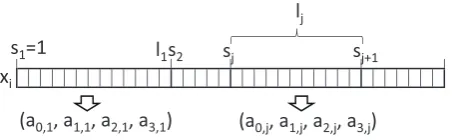
To illustrate the relation between the raw data in a time sequence of values and the compressed parameter sets, Fig. 2 shows an illustration of TOKI compression with third-degree polynomials.

Fig. 2 Illustration of TOKI compression using third-degree polynomials.

2.2 TOKI compression with Chebyshev

ap-proximation

Instead of the least-squares method discussed above, we can use Chebyshev approximation [14] to ﬁnd the co-eﬃcients ofkth-degree polynomials. Chebyshev polyno-mials, which are orthogonal polynopolyno-mials, are used to ex-pand the particle trajectories. A Chebyshev approximation is similar to the minimax approximation that minimizes the

maximumerror within an interval, while the least squares method minimizes theaverageerror. Therefore, Cheby-shev polynomials are more favorable for satisfying condi-tion (1) and, as a result, the intervals of trajectories can be made longer.

Chebyshev polynomials are deﬁned by

Tn(x)=cos(narccosx), (3)

wherenis an integer. With these polynomials, a function

f(x) can be approximated by a Chebyshev expansion

f(x)=

n

anTn(x). (4)

The coeﬃcients in this expansion are determined from the following integral formula, which is similar to that of a Fourier expansion:

an=

2 π

1

−1

f(x)√Tn(x)

1−x2dx. (5)

This integral can be calculated by direct numerical integra-tion or by evaluating the integrand at predetermined sam-ple points. Many numerical library programs support the latter method.

2.3 Test data from a PIC simulation

(4)

where c denotes the speed of light. The ratio of ion mass to electron mass was 100. Periodic boundary con-ditions were employed, and the simulation box size was 3.85c/ωce×1.92c/ωce×3.08c/ωce, whereωceis the elec-tron cycloelec-tron frequency. We set the numbers of grids for ﬁeld variables (electromagnetic ﬁeld, charge and cur-rent densities) to 16×15×16 as a test case. Based on the CFL (Courant–Friedrichs–Lewy) condition, ΔtCFL = (0.5/c) min(dx,dy,dz) was used to avoid numerical insta-bilities. To obtain smooth particle trajectories, we set the sampling rate toΔtsampling =0.016/ωce, which is a quarter ofΔtCFL=(0.5/ωce) min(3.85/16,1.92/15,3.08/16).

3. Results

3.1 TOKI compression with least-squares

method

We examined the eﬀects of the length of work array

Lwork and allowed errorε. To ﬁnd the longest interval for polynomials, the bisection method was used for speed in the ﬁrst implementation of the code. We measured the ra-tio of compressed data size to original data size; the latter is given by the size of all data in double precision binary format, that is, 8 bytes×24,000 for one particle. For this paper, the compressed data size was calculated in the as-sumed data format to avoid the overhead involved in ex-tracting data from the given format. Here, we recorded the compressed data of a certain interval in the following for-mat:

1) start time: integer (4 bytes)

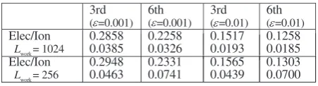
2) number of compressed data points: integer (4 bytes) 3) coeﬃcients of polynomials: double (8 bytes×(k+1)) Table 1 shows compression ratios forLwork=256 and 1024, and forε=0.001 and 0.01. It is clear that the size of the work array and the value of the allowed error both impact the compression ratio. It is found that relative size becomes smaller for higher degree polynomials for large

Lwork. By using a higher degree polynomial for ﬁt, al-though the number of coeﬃcients to express a polynomial in each interval, (k+1), increases, the length (number of data points) of each interval, lj, generally increases, too.

This decreases the number of intervals for a particle tra-jectory. Therefore, the total size of the compressed data (the number of coeﬃcients of the polynomial in an inter-val times the number of interinter-vals for the trajectory) can be smaller depending on the characteristic of the trajec-tory. It denotes existence of optimal degree for given data set. We can see that the optimal degree of ions’ trajec-tories is less than 6 forLwork =256 and those of other-wise are not less than 3. We considered the optimal de-gree is related to behaviors of each particle. It is consid-ered that given simulation conditions determine the opti-mal degree as well as behaviors of each particle. Although higher degree seems to be better for largeLwork, there is also a trade-oﬀin computing costs (elapsed time of

com-Table 1 Relative sizes of compressed data ﬁles using third- and sixth-degree polynomials.

pression). For sixth-degree polynomials, the Householder method (before optimization) was used in our implemen-tation. This method is much slower than direct solution for the third-degree polynomials.

Table 1 shows that the relative sizes of compressed data for ions are much smaller than those for electrons; this is because the motions of ions are relatively slow and the trajectories are smoother due to the diﬀerence in mass. In the simulations, the mass of ions was 100 times that of electrons. From a rough estimate based on the square root of the mass ratio, we expected the size of compressed data for electrons to be 10 times that for ions. ForLwork= 1024, the obtained results are almost consistent with this rough estimation. However, this is not the case forLwork= 256. We think the reason is the shortness ofLwork. Details of eﬀects of work array lengthLworkon compression ratio should be examined in the future.

3.2 TOKI compression with Chebyshev

ap-proximation

As another test for efficient compression by the TOKI scheme, we tried Chebyshev approximation. To find the coefficients of the polynomials in this method, we used the library function gsl_cheb_eval_n_err() from the GNU Sci-entific Library [16]. This function approximately employs the sample points method mentioned in Sec. 2.2. In this function, we can change the degree of polynomials and set the maximum degree of polynomials,kmax. For points in the range [a,b] and for the allowed error ε, we can use this library function to obtain the degree and coefficients of Chebyshev polynomials. In this preliminary implemen-tation, we estimated the error in Chebyshev approxima-tion withkmax-th degree polynomials and given maximum lengthLwork for trial. When this error is smaller than the allowed errorε, we seek the polynomial of lowest degree,

k, that satisﬁes condition (1) on the error. Otherwise, we ﬁnd the largest length for thekmax-th degree polynomial.

We examined how the size of the compressed data is aﬀected by the length of the work arrayLworkand the maxi-mum degree of Chebyshev polynomialskmax. We recorded the compressed data of a certain interval in the following format:

1) start time: integer (4 bytes) 2) length of this interval (4 bytes)

(5)

Table 2 shows relative sizes of compressed data ﬁles forLwork =256, 1024, and 4096, and forkmax=3, 6, 10, 20, and 40. Here, we setε=0.001. The table shows that the compressed sizes using Chebyshev approximation are smaller than those for the usual polynomials with the least-squares method discussed in Section 3.1 (compare with Ta-ble 1).

For largekmaxandLwork, the relative size of the com-pressed file becomes smaller. For large kmax and large Lwork, the relative size becomes smaller. For large kmax and small Lwork, no difference occurs between electrons and ions, while a difference does appear for largeLworkand kmax. These behaviors of relative size for value ofkmax de-note existence of optimal value ofkmax for given data set, Lworkand our implemented algorithm. More details should be examined in the future.

It is noted that algorithm to choose length lj

(num-ber of data points) and degreekof Chebyshev polynomials should be modified in order to obtain smallest file size. Al-though the algorithm of the present paper selected lowest degree for fixedLworkor largestljfor fixedkmax, we should find pair ofkandljto minimize value ofk/lj. For this

mod-iﬁed algorithm, computing cost becomes too much because computation of many pairs ofkandljis required.

3.3 Comparison with other compression

schemes

Sections 3.1 and 3.2 show that the relative size of a compressed data ﬁle depends on features of particle trajec-tories. Thus, we expect that the relative size of compressed data can be used as a representative parameter to categorize trajectories. So, we used other compression methods to test whether this idea is valid. Here, we checked the XTC for-mat [4], which is widely used as a compression method for trajectory data in particle systems.

The sampling rateΔtsamplingis an important parameter

Table 2 Relative sizes of compressed ﬁles by Chebyshev ap-proximation forε=0.001.

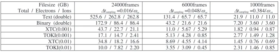
Table 3 Comparisons of sizes of compressed ﬁles from XTC and TOKI.

in TOKI compression becauseΔtsamplingis directly related to the smoothness of the trajectories. We checked the eﬀect ofΔtsampling on the compression eﬃciency for both TOKI compression and the XTC format.

The data for 24,000 time steps of three-dimensional positions for 300,000 particles requires about 525 GB in Fortran double-precision text format. For 30 frames/s, this corresponds to 657 MB/s, which is faster than SSD. Ta-ble 3 shows the sizes of compressed ﬁles from the XTC and TOKI schemes (with the least-squares method) at two precisions indicated by decimals 0.001 and 0.01. In the XTC format, trajectories were written as a diﬀerence of bits of rounded integers multiplied by a scale factor (typi-cally 1000 for 0.001 accuracy).

When the time intervalΔtsamplingis smaller thanΔtCFL, the TOKI scheme shows a good compression ratio. For smooth trajectories (Δtsampling ΔtCFL), the ratio for TOKI is much better than that for the XTC format. However, for ballistic trajectories (Δtsampling ΔtCFL), the compression ratio for TOKI is not good because of the overhead associ-ated with storing raw values of trajectories. We found that the size of TOKI compressed ﬁles depends on the motion of each particle, while the size for XTC is almost propor-tional to the number of frames and is independent of the motion of each particle. From this, we expect that the be-havior of the compression ratio for TOKI can be used as a characterization parameter for particle motions.

4. Conclusions

(6)

is due to the diﬀerence in mass. We expect that the be-havior of the compression ratio from TOKI can be used to characterize the motions of plasma particles. In future work, distribution of TOKI software as a system software library will be considered. Studies toward this goal are in progress.

Acknowledgements

This work is partly supported by “Joint Us-age/Research Center for Interdisciplinary Large-scale Information Infrastructures” (JHPCN-HPCI Project ID: jh130038, hp130062, and hp130122) in Japan, NIFS/NINS under the project of Formation of International Scientiﬁc Base and Network, and HPC project of Nagoya Univer-sity. The authors thank Dr. A. M. Ito, Dr. T. Takeda, and Dr. T. Saito for useful discussions at early stage of this work under National Institutes of Natural Sciences (NINS) Program for Cross-Disciplinary Study.

[1] C.K. Birdsall and A.B. Langdon,Plasma Physics Via

Com-puter Simulation(McGraw-Hill, New York, 1985). [2] F.F. Chen,Introduction to Plasma Physics(Plenum Press,

New York, 1974).

[3] W. Horton and T. Tajima, J. Geophys. Res. 96, 15811 (1991).

[4] A. Ishizawa and R. Horiuchi, Phys. Rev. Lett.95, 045003 (2005).

[5] W. Daughtonet al., Nature Physics7, 539 (2011). [6] T. Sugiyama, Phys. Plasmas18, 022302 (2011).

[7] M.A. Riquelme and A. Spitkovsky, Astrophys. J.733, 63 (2011).

[8] Y. Matsumotoet al., Astrophys. J.755, 109 (2012). [9] http://www.hdfgroup.org/

[10] D.G. Green, K.E. Meacham, M. Surridge, F. van Hoesel and H.J.C. Berendsen, Metecc-95 Proceedings (1955). [11] http://www.gromacs.org/

[12] D. Spangberg, D.S.D. Larsson and D. van der Spoel, J. Mol. Model17, 2669 (2011).

[13] H. Ohtani, K. Hagita, A.M. Ito, T. Kato, T. Saitoh and T. Takeda, J. Phys: Conf. Ser.454, 012078 (2013).

[14] R.W. Hamming,Numerical Methods for Scientists and En-gineers, second edition (McGraw-Hill, New York, 1973). [15] E.G. Harris, Nuovo Cimento23, 115 (1962).